Approximate methods in Bayesian point process spatial models

Abstract

A range of point process models which are commonly used in spatial epidemiology applications for the increased incidence of disease are compared. The models considered vary from approximate methods to an exact method. The approximate methods include the Poisson process model and methods that are based on discretization of the study window. The exact method includes a marked point process model, i.e., the conditional logistic model. Apart from analyzing a real dataset (Lancashire larynx cancer data), a small simulation study is also carried out to examine the ability of these methods to recover known parameter values. The main results are as follows. In estimating the distance effect of larynx cancer incidences from the incinerator, the conditional logistic model and the binomial model for the discretized window perform relatively well. In explaining the spatial heterogeneity, the Poisson model (or the log Gaussian Cox process model) for the discretized window produces the best estimate.

1. Introduction

Analyzing case event data in spatial epidemiology with residential locations (also known as spatial point patterns) is gaining more importance. The advantage of this approach is that the analysis incorporates the geographical location of events of interest which helps to reduce the model variance and leads to a correct inferential procedure. This paper aims to review some of the point process models that are commonly used in relation to the assessment of the effects of putative sources of hazard for the increased incidence of disease and to compare their relative performances when the true parameter values are known. We also mention the differences in interpreting the distance effects for each of these models. The approximate methods include the Poisson process model and the methods that are based on discretization of the study window. The exact method is based on a marked point process model, i.e., a conditional logistic model. The paper also addresses the issue of flexible modeling by demonstrating the use of approximate likelihood and Bayesian models, and their posterior sampling.

In analyzing case event data, the theoretical advancement has outmatched ready-to-use software. While routines now have appeared in, for example, the R package (R Development Core Team, 2004), that allow testing or simple modeling (e.g. DCluster (Gómez-Rubio et al., 2004), Spatstat (Baddeley and Turner, 2005), Splancs (Rowlingson and Diggle, 1993)), there is limited availability of algorithms that can be implemented easily for more sophisticated analyses with covariates. This is partly due to the fact that the basic likelihoods, e.g. the non-homogeneous Poisson process, involve normalizing constants that must be evaluated. There is a demand for flexible approaches to the modeling of case event data that can allow for the inclusion of covariates (spatially referenced or otherwise). Another advantage would be to have the extra flexibility of a Bayesian hierarchical modeling approach to case event data. These needs mirror the developments of Bayesian methods and software for count data (see e.g. Congdon (2003) and Lawson et al. (2003)). The implementation of all the methods, approximate and exact, described in this paper is via WinBUGS (Spiegelhalter et al, 2003), and hence the full range of Bayesian modeling machinery within that package is potentially available.

The organization of this paper is as follows. In the next section, we give a brief illustration of all the methods that are considered in this paper to analyze a point process dataset. In this illustration, we describe the point process models with the Berman and Turner (1992) proposal of weighted sum approximation to an integral in the likelihood (see also Lawson (1992)), the conditional logistic models (Diggle and Rowlingson, 1994), and very briefly, the grid mesh construction. The details of the Poisson mesh model and binomial mesh model approaches, based on the discretization of the study window, are introduced in Section 5. Although the discretization approach to case event data (or point process data) in epidemiological studies is quite common, we illustrate the theoretical justification and the assumptions involved in that approach. The Lancashire larynx cancer data are used in relative comparison and the data are introduced in Section 3. In Section 4, we introduce two random components in the specification of intensity function and define their distributions in a Bayesian setting. Section 6 illustrates the larynx cancer data analysis and results. The simulation technique and results are given in Section 7 and the concluding remarks are in Section 8.

2. Methods for analysis of point process data

A brief illustration of likelihood models and the conditional logistic model is given in this section, followed by a brief introduction of alternative methodology based on grid meshes. The adopted notations are as follows.

Suppose that the geographical study region, A, is given within which we intend to describe the spatial distribution of disease of a population. The data are represented by a set of locations s_i ∈ A, i = 1, …, n for cases and c_j ∈ A, j = 1, …, m for controls. For the models that we consider, cases and controls form a pair of independent, inhomogeneous Poisson point processes, with respective intensities, at the data locations, λ(s) and λ₀(c) where the vectors s = (s₁, …, s_n)^T and c = (c₁, …, c_m)^T.

2.1. Point process models

The number of cases follows a Poisson distribution with expectation μ_A = ∫_A λ(s)ds. Conditional on the number of cases, n in A, case locations are an independent random sample from the distribution on A with probability density proportional to λ(s). The unconditional likelihood of a realization of n cases is given by

$$L=\prod _{i=1}^n\lambda ({\mathbf{s}}_i)exp\left(-{\int }_A\lambda (\mathbf{s})\text{d}\mathbf{s}\right).$$ (2.1)

The intensity function, λ(s), can be defined to include a modulating function which can represent the background population, and also covariate information. We assume that the cases are governed by a first-order intensity of the general form

$$\lambda (\mathbf{s})=\rho {\lambda }_0(\mathbf{s})\theta (\mathbf{s}),$$ (2.2)

where θ(s) is the relative risk at the location s including all the covariates and has a parametric form, λ₀(s) represent the background population effect at s, and ρ is a scaling parameter reflecting the overall incidence of cases relative to the region of controls. When θ(s) = 1, ρ is the scaling factor of the two intensities.

Integration schemes

Berman and Turner (1992) proposed a quadrature rule to approximate the integral in (2.1) which makes feasible the estimation of model parameters in a GLM framework. We call this method the BT method. Following the rule, the integral in (2.1) is approximated as

$${\int }_A\lambda (\mathbf{s})\text{d}\mathbf{s}\doteq \sum _{k=1}^N{\omega }_k\lambda ({\mathbf{s}}_k),$$

where s_k, k = 1, …, N, are points in A including all the data points {s_i, i = 1, …, n} and (N − n) dummy points. The quadrature weights, ω_k > 0, are calculated such that ${\sum }_{k=1}^N{\omega }_k=\mid A\mid$. It is recommended to consider a reasonably large N to minimize the quadrature error. With this approximation, the log-likelihood of (2.1) can be written as

$$l=\sum _{k=1}^N{\omega }_k\{\frac{I_k}{{\omega }_k}log\lambda ({\mathbf{s}}_k)-\lambda ({\mathbf{s}}_k)\}$$

where I_k is an indicator function, which takes the value 1 if s_k is a data point, and otherwise 0. The above log-likelihood function is similar to a weighted Poisson log-likelihood with Poisson variable {I_k/ω_k} and parameter λ(s_k), which is equal to ρλ₀(s_k) θ (s_k).

2.2. An alternative likelihood: The conditional logistic model

Instead of considering the population to be described as a pair of Poisson processes, we can think of it as a single marked point process with a common intensity (Diggle and Rowlingson, 1994). A random variable Y_i (i = 1, …, n + m) can be defined for each location, which takes the value 1 or 0 depending on whether the i-th location is a case or control. Now, the probability that location i is a case is given by

$$p_i=\frac{\lambda ({\mathbf{s}}_i)}{{\lambda }_0({\mathbf{s}}_i)+\lambda ({\mathbf{s}}_i)}=\frac{\rho \theta ({\mathbf{s}}_i)}{1+\rho \theta ({\mathbf{s}}_i)}.$$

In likelihood construction, the data are now treated as a binary marked observation rather than a point process. An immediate advantage of this approach is that the integral of (2.1), and hence the approximation, are no longer required. The log-likelihood takes the form

$$\sum _{i=1}^{n+m}\{y_{i}log{\phi }_i-log(1+{\phi }_i)\},$$

where φ_i = ρθ (s_i). This conditional logistic model is called the CL model hereafter.

2.3. Grid mesh constructions

While it is possible to utilize these models directly, alternative approximate approaches may also be useful. Here we use an alternative method consisting of dividing the study area into a number of smaller mesh cells. Based on the count of number of points in each cell a conditional Poisson or binomial model can be fitted as a Bayesian hierarchical model where correlation is admitted at a higher level of the hierarchy. Standard errors and credible intervals of estimates and also model goodness-of-fit statistics, e.g. deviance, DIC (deviance information criteria) or PPL (posterior predictive loss) are readily available. A big advantage of this approach is that all the models could be implemented within available software (e.g. WinBUGS, which would make available for use a rich variety of MCMC sampling machinery). The incorporation of certain types of spatial association into models in WinBUGS is also straightforward.

3. Larynx cancer data

We consider a particular data example, Lancashire larynx cancer data (Diggle, 1990), to illustrate all the methods considered in this paper. The data include the residential location of larynx cancer deaths (58 cases), recorded in the Chorley and South Ribble Health Authority of Lancashire during 1974–83. The objective in that work was to assess the evidence of increased larynx cancer incidence near an industrial incinerator, which was suspected as a possible source of health hazard. As a control variable, the author considered lung cancer deaths (978 controls) for the same period in the same study area. Fig. 1 displays the locations of cases, controls and incinerator. The units of co-ordinates are given in 10 m.

Fig. 1.

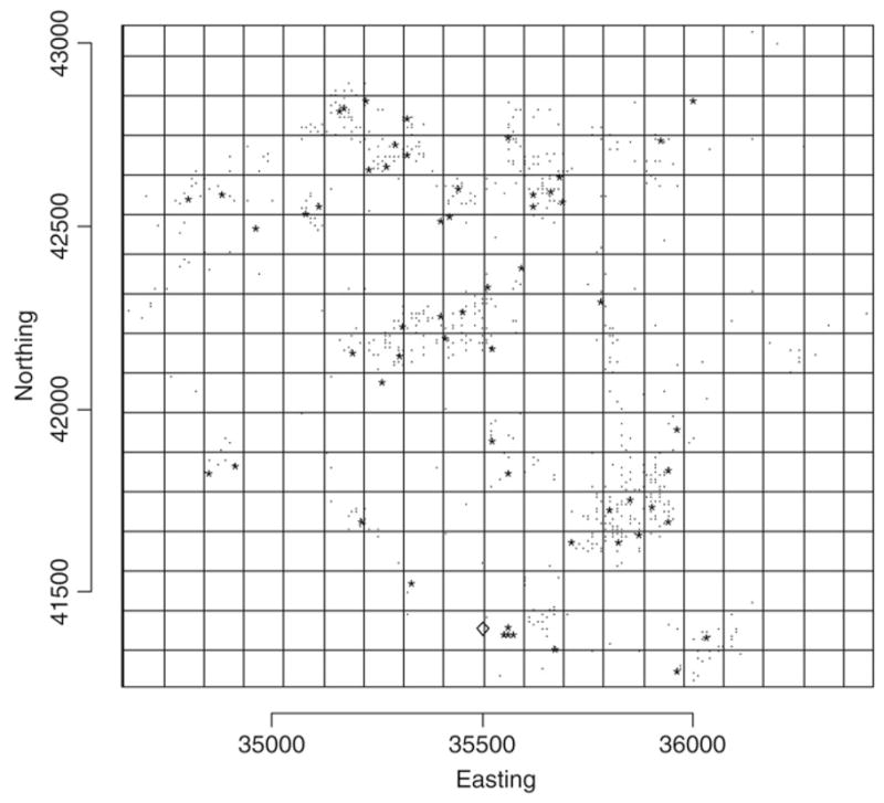
Larynx cancer as case denoted by “*”, lung cancer as control denoted by “.”, and “◇” the incinerator location with grid mesh.

In all our model development discussed later, we consider distance from the source as the only spatially derived covariate. It is straightforward to include other important covariates, e.g. direction, in these models. Also, in more generality, a range of covariates could be included. However, for simplicity of presentation we confine the discussion only to the distance effect, which is of main interest in the assessment of the incinerator effect on increased number of larynx cancer cases.

4. Random effects in Bayesian point process models

Whenever a likelihood function is available, it is possible to use a Bayesian paradigm to provide a posterior distribution for all unknown parameters. It is reasonably straightforward to assign prior distributions for all the unknowns in the above intensity function (2.2). In what follows we will examine Bayesian extensions to this and other likelihoods and assign suitable prior distributions to relevant parameters. We will give the detailed specification of prior distributions for each model below.

The relative risk at point s_i, θ (s_i), can now be modeled with a variety of model specifications. We consider a multiplicative model, to assess the distance effect on larynx cancer cases in the presence of a single putative hazard source, of the form

$$\theta ({\mathbf{s}}_i)=g(d_i,\mathit{\beta })exp({\mathbf{z}}_i^{\text{T}}\mathit{\gamma })$$

where d_i is the distance of the i-th point from a putative hazard source, z is a set of covariates thought to include all the confounder information, and the dimension of coefficient vector γ depends on the number of confounders. Diggle et al. (1997) proposed an additive risk model for g (d_i, β) of the form (1 + f(d_i, β)). However, this form has identifiability problems (at least computational identifiability) and so we do not use this form here (see e.g. Ma et al. (2007)). Instead we opt for a multiplicative model. The distance effect is modeled as

$$g(d_i,\mathit{\beta })=exp\{{\beta }_0+{\beta }_1{d}_i\},$$

where β₀ is the intercept and β₁ measures the distance effect. In the case of multiple putative hazard sources, the above expression can be extended to add an individual source distance with a coefficient to measure their effects on disease incidence.

In the intensity specification, in the model for θ (s), it is possible to include random effect terms that can allow for extra variation in the rate of the process. These effects are often specified with a log link to the risk to ensure positivity. For example, $z_i^{\text{T}}\gamma =v_i+u_i$ could be specified where v_i and u_i are two spatially referenced heterogeneity terms. This leads to the formulation

$$log{\theta }_i={\beta }_0+{\beta }_1{d}_i+v_i+u_i.$$

The two random effects, v_i and u_i, are intended to incorporate spatial and non-spatial heterogeneity into the model. These terms are commonly assumed within Bayesian mapping models (see e.g. Besag et al. (1991)). The modeling of the correlated random variable v = (v₁, …, v_N)^T can proceed either by specifying the joint distribution of v or by univariate conditional distributions [v_i |{v_j}], i ≠ j, i = 1, …, N.

In setting the prior distribution for correlated random effects, we consider the conditional distribution approach and use the CAR (conditional autoregressive distribution) model, which is defined as a series of univariate conditional distributions [v_i|{v_j}], i ≠ j, i = 1, …, N. Following Besag et al. (1991), this is given as

$$v_i\mid \{v_j\},m_i,{\sigma }_v^2\sim \text{N}\left({\overline{v}}_i,\frac{{\sigma }_v^2}{m_i}\right),$$

where $m_i={\sum }_{j=1}^{N}I(j\in \{{\delta }_i\}),{\overline{v}}_i={\sum }_{j\in \{{\delta }_i\}}\frac{v_j}{m_i}$, {δ_i} is the set of first-order neighbors (the regions which share common geographical boundaries with i-th region) of the i-th point, I (·) is an indicator function, which takes the value 1 if the condition within parentheses is satisfied, and is otherwise 0, and ${\sigma }_{\nu }^2$ is a spatial correlation parameter. The first-order neighborhood can be found, for example, from a Dirichlet tessellation for a point process.

For the other random effect, u_i, which models heterogeneity arising from uncorrelated noise, we assume an exchangeable normal distribution with zero mean and variance ${\sigma }_u^2$.

5. Methods based on grid mesh

In this section we illustrate a novel approach to the analysis of point pattern data. The methodology is based on the use of discretization of the study window into a grid mesh. A map of a study area can be of any shape. It is possible to split a map into a grid system of regular cell sizes, e.g., into a number of equal rectangular meshes if the study region is rectangular. That is, for a rectangular study area we consider disjoint sets {A_k}, k = 1, …, K, whose union is A, such that |A_k| > 0 are similar for all k. Fig. 1 displays the Lancashire larynx cancer study map: a rectangle map split into equal sizes of rectangular meshes.

The points of the observed processes (case and control) are binned into the cells and a mesh of cell counts results. If any point is on the grid line of two meshes, it is counted in either of the meshes at random. Given the counts observed within meshes, a likelihood can be constructed which describes the probability of counts observed within the cells. Possible choices of models could be Poisson or binomial depending on whether the disease is rare or non-rare.

5.1. Poisson mesh model

Let the map be split into K cells: A_k(k = 1, …, K) is the k-th cell of map (window) A, $n_k^{\text{case}}$ and $n_k^{\text{control}}$ are the number of cases and controls in A_k, respectively. The total count in cell k is $n_k=n_k^{\text{case}}+n_k^{\text{control}}$. Following Section 2.1, the number of cases in A_k, $n_k^{\text{case}}$, follows a Poisson distribution with mean

$${\mu }_k^{\text{case}}={\int }_{A_k}\lambda (\mathbf{u})\text{d}\mathbf{u}={\int }_{A_k}\rho \theta (\mathbf{u}){\lambda }_0(\mathbf{u})\text{d}\mathbf{u},\forall k.$$

If we assume that all of the variables in θ (u) are constant within each cell A_k, then the means are

$${\mu }_k^{\text{case}}=\rho {\theta }_k{\int }_{A_k}{\lambda }_0(\mathbf{u})\text{d}\mathbf{u},\forall k.$$

For reasonably large numbers of mesh cells, the effect of this assumption is negligible. The remaining integral on λ₀ can be replaced by background (or control) population estimates. Commonly, it is replaced by a case-mix adjusted expected count for the k-th cell. Diggle (2000) proposed replacing the above integral by its unbiased estimator, the population size within cell A_k. For this specific dataset, we propose replacing the above integral by n_k, the total number of cases and controls within cell A_k. It is important to mention that the Lancashire larynx cancer dataset contains only the case-control indicators with their geographical locations. Hence, replacing the integral by n_k is a reasonable choice in this situation. Thus at the first level of hierarchy, we have a Poisson model as

$$n_k^{\text{case}}\sim \text{Poisson}({\mu }_k^{\text{case}})$$

and, at the second level, a log-linear model gives

$$log({\mu }_k^{\text{case}})=log(n_k)+log\rho +{\beta }_0+{\beta }_1{d}_k+v_k^{\text{case}}+u_k^{\text{case}},$$

where d_k is the distance of the centroid of k-th cell from the putative hazard source (a fixed point). Two random effects, u^case and v^case, are included, and these represent unstructured and structured heterogeneity, respectively.

In a similar argument, we can conclude that the number of controls in the k-th cell, $n_k^{\text{control}}$, follows a Poisson distribution with mean

$${\mu }_k^{\text{control}}={\int }_{A_k}{\lambda }_0(\mathbf{u})\text{d}\mathbf{u},\forall k.$$

As before, the above integral can be replaced by n_k. In addition to n_k, we also add two random effect terms in order to include heterogeneity. Thus, for controls, at the first level of hierarchy, we fit a Poisson model as

$$n_k^{\text{control}}\sim \text{Poisson}({\mu }_k^{\text{control}})$$

and, at the second level as

$$log({\mu }_k^{\text{control}})=log(n_k)+v_k^{\text{control}}+u_k^{\text{control}}.$$

Two random effects, u^control and v^control, are included and these represent unstructured and structured heterogeneity, respectively.

A number of models can be formulated based on common structured heterogeneity (SH) and/or common unstructured heterogeneity (UH) of case and control counts. Common SH will leads to a correlated model. We can choose the nature of random effects to include by assessing model goodness-of-fit. The DIC (a model selection criterion) (Spiegelhalter et al., 2002) can be used, which selects the most parsimonious model among those fitted after penalizing for model complexity.

5.2. Binomial mesh model

For a non-rare disease, instead of the Poisson distribution at mesh level, a binomial distribution can be fitted. Let n_k be the total number of points in cell k, i.e., $n_k=n_k^{\text{case}}+n_k^{\text{control}}$. Thus at the first level of the hierarchy, we have

$$n_k^{\text{case}}\sim \text{Binomial}(p_k^{\text{case}},n_k),$$

where $p_k^{\text{case}}$ is the probability that the k-th cell has $n_k^{\text{case}}$ cases. A logit link function will lead to

$$\text{logit}(p_k^{\text{case}})=log\rho +{\beta }_0+{\beta }_1{d}_k+v_k^{\text{case}}+u_k^{\text{case}}$$

and the hierarchical model can be specified at higher levels as in Section 5.1.

In short, we call these models the PM model for the Poisson mesh model and the BM model for the binomial mesh model.

5.3. Connection between PM model and the log Gaussian Cox process

Moller et al. (1998) gave a detail description of the log Gaussian Cox process (LGCP) and its properties. A Cox process X is a point process with random intensity λ such that X|λ is a Poisson process with intensity function λ. For an LGCP, the random intensity function is given by λ = exp(Z), where Z is a Gaussian field on A for which the random intensity measure μ_A = ∫_A exp(Z(s))ds.

After discretizing the observation window A into K disjoint cells {A_k} similarly as for grid meshes, the count of realized cases $n_k^{\text{case}}$ will follow a Poisson distribution with mean $exp({\chi }_k^{\text{case}})$, where ${\chi }_k^{\text{case}}$ is a realization of Z (s_k). It is clear from this discretization that the LGCP model is similar to the PM model when $exp({\chi }_k^{\text{case}})={\mu }_k^{\text{case}}$. Thus, the realized value has the form

$${\chi }_k^{\text{case}}=log(n_k)+log\rho +{\beta }_0+{\beta }_1{d}_k+v_k^{\text{case}}+u_k^{\text{case}}.$$

Rue et al. (submitted for publication) adopted a similar discretization approach to an LGCP (see also, Waagepetersen (2003)).

5.4. Interpreting the distance effects of each of these models

For the specific parameterization of the intensity function that we have illustrated in Section 4, the regression coefficient (β₁) for the distance effect on disease incidence should be interpreted cautiously for each model. This is mainly because of the distinctness of the assumed probability distribution and the formulation at the first level of hierarchy.

For the CL and the BM models, β₁ measures the average effect of distance from the incinerator for a probability of disease occurrence on a logit scale. In the case of the BT model, β₁ measures the average effect of distance on the ratio of case and control intensities on a log scale. Generally, it measures the changes in SMR (standardized mortality ratio). The interpretation of β₁ for the PM model will depend on the approximation used for the integral on λ₀. If this integral is replaced by a case-mix adjusted expected count, the β₁ in the PM model will have a similar interpretation as for the BT model. In the Lancashire larynx cancer data, we replace this integral by the total count of cases and controls for each cell; the β₁ in PM model will have a similar interpretation as for the CL and BM models.

6. Data example

In the implementation of the BT method, we have considered 462 points, out of which 58 are case points and 404 are dummy points (400 centroids of 20 × 20 grid meshes and 4 corner points). The role of dummy points is to increase the precision of integration scheme. To estimate the unknown control intensity λ₀ (x_j), we use the “sm.density” function in R to get a nonparametric density estimates for controls, and then rescale it by multiplying the density estimates by m (the total number of controls) to get an estimate of the intensity function, λ̂₀, at each point x_j. Note that dividing the intensity by its integral over A yields the density. We plug in these estimates in the likelihood function to get estimates of all other unknown parameters: ρ, β₀, β₁, σ_u, and σ_v.

As in other methods, 1036 binary points are considered for the CL method and 900 cells are constructed for the grid methods, although a comparison has been made with a smaller number of cells (400) within grid methods to observe changes in estimates for mesh size changes. In the implementation of all the methods, we use the CAR prior distribution for the correlated random effect v_i. The adjacent points for the BT and CL methods are obtained by the Dirichlet tessellation method (Okabe et al., 2000). Dirichlet tessellation is a process of dividing an area into smaller, contiguous non-overlapping tiles, one per data point, with no gaps in between them. The i-th tile contains all spatial locations that are closer to the i-th data point than any other data point. We used the R function (provided by Rolf Turner on request) to get the polygons of the Dirichlet tessellation tiles. A map of tiles in WinBUGS based on these polygons yields an adjacency matrix of neighbors.

In the implementation of the BM model, a difficulty arises when we observe that many n_i’s are counted as zero. This means that some cells have zero total count. To circumvent this problem we adopt an ad hoc measure proposed in http://www.mrc-bsu.cam.ac.uk/bugs/faqs/lavine.shtml. The idea is developed as follows.

A vector, ξ_k, for each k of order C is introduced with the elements

$${\xi }_{k1}=I(n_k=0)+I(n_k=1)$$

and,

$${\xi }_{kj}=I(n_k=j),$$

where j = 2, …, C and C is set to the maximum value of n. The elements of vector ξ_k will have one 1 and (C − 1) zeros. Now, a new n_k is generated as

$$\mathit{new}.n_k\mid {\mathit{\xi }}_k\sim \text{Categorical}({\mathit{\xi }}_k).$$

In order to ensure that $p_k^{\text{case}}$ is zero whenever n_k is zero, a new $p_k^{\text{case}}$ is introduced as

$$\mathit{new}.p_k^{\text{case}}=p_k^{\text{case}}(1-I(n_k=0)).$$

Now, the binomial model appears as

$$n_k^{\text{case}}\sim \text{Binomial}(\mathit{new}.p_k^{\text{case}},\mathit{new}.n_k).$$

The sampling from the above binomial (sometimes called phony binomial) distribution is feasible since the new.n_k’s are non-zero; at the same time, this approach also enforces $\mathit{new}.p_k^{\text{case}}$ equal to zero whenever n_k is zero. For non-zero n_k, the effect of this approach is insignificant since new.n_k and n_k are equal for those k. Another alternative approach could be zero-inflated Poisson regression (Agarwal et al., 2002), where n_k is assumed to have a distribution. However, in subsequent analysis we adopt the former approach.

6.1. Results

Table 1 gives the results obtained by each method for each parameter, β₀, β₁, log (ρ), σ_u, and σ_v. We use the software WinBUGS, run for 120,000 iterations with first 100,000 as burn-in. The estimates are given with 95% credible intervals (CI’s) in parentheses. The regression coefficient, β₁, indicates the distance (from the incinerator) effect on larynx cancer cases. The estimates of β₁ from all the methods are very close, and the 95% CI’s indicate that the effect is insignificant. Among the intercept estimates, the CL method produces the largest estimate with the widest confidence band and the BM model for the mesh size 20 × 20 produces the smallest estimate with the narrowest confidence band. The BT method produces the largest variability estimate for the spatially correlated random effects and the smallest variability estimate for the uncorrelated random effects.

Table 1.

Posterior mean estimates (95% credible intervals are given in parentheses) from the BT, CL and grid mesh methods for larynx cancer data

Parameter	BT method	CL model	PM model		BM model
			20 × 20	30 × 30	20 × 20	30 × 30
β0	0.887 (−0.608, 2.386)	−1.532 (−3.132, 0.063)	−1.294 (−2.737, 0.121)	−1.266 (−2.662, 0.110)	−1.133 (−2.336, 0.100)	−1.155 (−2.657, 0.226)
β1	−0.00043 (−0.00176, 0.00089)	−0.00059 (−0.00255, 0.00042)	−0.00032 (−0.00123, 0.00047)	−0.00048 (−0.00135, 0.00036)	−0.00070 (−0.00204, 0.00040)	−0.00058 (−0.00156, 0.00029)
log(ρ)	0.998 (−0.403, 2.470)	−1.270 (−2.980, 0.297)	−1.341 (−2.662, 0.058)	−1.273 (−2.790, 0.197)	−1.156 (−2.509, 0.313)	−1.247 (−2.584, 0.232)
σu	0.133 (0.006, 0.659)	0.877 (0.183, 2.733)	0.221 (0.011, 0.616)	0.303 (0.035, 0.675)	0.266 (0.010, 0.643)	0.349 (0.054, 0.771)
σv	1.365 (0.460, 2.785)	0.546 (0.119, 1.608)	0.297 (0.012, 1.212)	0.661 (0.238, 1.240)	0.869 (0.244, 1.817)	0.700 (0.176, 1.602)

Two mesh sizes, 20 × 20 and 30 × 30, were considered for PM and BM models to check the mesh-size effect on the estimates. The results vary a little for mesh sizes for the estimates of β₀, β₁ and log (ρ). For both mesh models, increasing the mesh size increases the variability of the uncorrelated random effects. The other noticeable change for the change in mesh size, the variability for the spatially correlated random effects, increases with the increase of the mesh size for the PM model, whereas for the BM model it decreases.

Table 2 gives results for the PM model for a 20 × 20 mesh size. We have considered four models depending on common and/or separate random effects for case and control models. The first model in column 2 considers no spatially correlated random effect for case and control, but has a separate uncorrelated random effect. The second model in column 3 considers separate spatially correlated random effects for case and control, and also has a separate uncorrelated random effect. The third model in column 4 considers a common spatially correlated random effect for case and control, but has a separate uncorrelated random effect. Note that this model considers a spatial correlation between case and control. The fourth model in column 5 considers a separate spatially correlated random effect but has a common uncorrelated random effect.

Table 2.

Posterior mean estimates from the PM model for larynx cancer data with 20 × grid meshes

	No v’s and separate u’s	Separate v’s and separate u’s	Common v’s and separate u’s	Separate v’s and common u’s
β0	−1.337 (−2.713, −0.005)	−1.158 (−2.714, 0.336)	−1.266 (−2.677, 0.245)	−1.211 (−2.648, 0.171)
β1	−0.00023 (−0.00091, 0.00043)	−0.00043 (−0.00143, 0.00033)	−0.00023 (−0.00088, 0.00041)	−0.00055 (−0.00155, 0.00031)
log(ρ)	−1.379 (−2.739, 0.013)	−1.391 (−2.871, 0.181)	−1.429 (−2.841, −0.068)	−1.217 (−2.652, 0.223)
σu	–	–	–	0.034 (0.005, 0.080)
σv	–	–	0.072 (0.014, 0.181)	–
${\sigma }_u^{\text{control}}$	0.024 (0.003, 0.072)	0.025 (0.002, 0.072)	0.034 (0.006, 0.075)	–
${\sigma }_u^{\text{case}}$	0.290 (0.046, 0.670)	0.198 (0.017, 0.566)	0.192 (0.017, 0.540)	–
${\sigma }_v^{\text{control}}$	–	0.043 (0.002, 0.146)	–	0.052 (0.001, 0.167)
${\sigma }_v^{\text{case}}$	–	0.515 (0.061, 1.377)	–	0.690 (0.088, 1.429)
DIC.case (pD)	198.72 (7.29)	198.68 (8.55)	197.76 (5.07)	198.39 (7.78)
DIC.control (pD)	512.35 (0.92)	513.91 (1.80)	516.23 (3.07)	515.32 (2.53)
DIC.total (pD)	711.06 (8.21)	712.60 (10.35)	713.98 (8.14)	713.72 (10.30)

For estimates, the 95% credible intervals, and for DIC the effective number of parameters are in parentheses.

All the estimates are given with 95% credible interval in parentheses. The DIC values are given with the effective number of parameters in parentheses. DIC.total is obtained by summing the DIC.case and DIC.control. The smallest DIC.total is obtained for the first model in column 2, which considers neither the case nor the control has a spatially correlated random effect but has a separate uncorrelated random effect. The DIC’s the for third and fourth models are very close, although each assumes quite different random effects for cases and controls. The smallest deviance (after subtracting the effective number of parameters from the DIC) without penalizing for extra parameters is obtained for the second model in column 3, which considers a separate spatially correlated random effect for case and control as well as a separate uncorrelated random effect.

7. Simulated data

We have also considered the performance of all these models in a simulation experiment whose purpose is to examine the ability to recover true parameter values. We generated a number of cases and controls for given values of all unknown parameters. These given values in the simulation experiment are known as true values.

A number of control data points and case data points are simulated separately within the Lancashire study area. Control points were generated from λ̂₀, a nonparametric estimate of intensity function for controls, in order to maintain a dependency on the original lung cancer data. All the steps of the simulation of control points are given in Appendix A. At step 1, estimates of the optimal smoothing parameters are obtained from “sm.density” function in R. At step 2, a random sample is drawn from the list of controls by using the “sample” function in R.

The parameterization that we have considered for the case intensity has the form λ_i = ρe^{β₀+β₁d_i}e^S_i, where S_i represents unexplained spatial variation. This S_i can also be thought of as a realization of a spatial stochastic process or, more generally, a Gaussian random field (GRF). Because of this representation of S_i, the spatially varying case intensity λ_i can also be interpreted as a log Gaussian Cox process (LGCP). Thus, S_i will have a nonstationary mean, log (ρ) + β₀ + β₁d_i.

Cases were simulated from an LGCP. The values for the parameters β₀ and β₁ are assumed as −1.0 and −0.005 to maintain similarities with the estimates from real data. The value for ρ is assigned as 1.0. All the steps of the simulation of case points are given in Appendix B. At step 3, r realizations of a GRF, S_i, were generated with the parameters, variance = 0.5, scale = 1.0 and nugget = 0.0 by using the R function “GaussRF”. The covariance function used in the random field generation takes the form of cov(S_i, S_j) = 0.5 exp(−d_ij). The values for the parameters (variance, scale, and nugget) are assigned accordingly to ensure small structural noise and points are uncorrelated for a small distance apart. Now, the cases are generated from the intensity function, λ_i = ρe^{β₀+β₁d_i}e^S_i, maintaining a similar parameterization as for real data.

We generate 200 controls and r realizations of 200 cases within the Lancashire study area. The numbers are chosen arbitrarily but purposely, to ensure equal number of cases and controls so that setting ρ = 1 is justified. In the case simulation, we set m_c = 10,000. The number of realization was set to 20, i.e., r = 20. Fig. 2 displays the simulated 200 controls (bottom-right cell) and 20 datasets of 200 cases (all except the bottom-right cell).

Fig. 2.

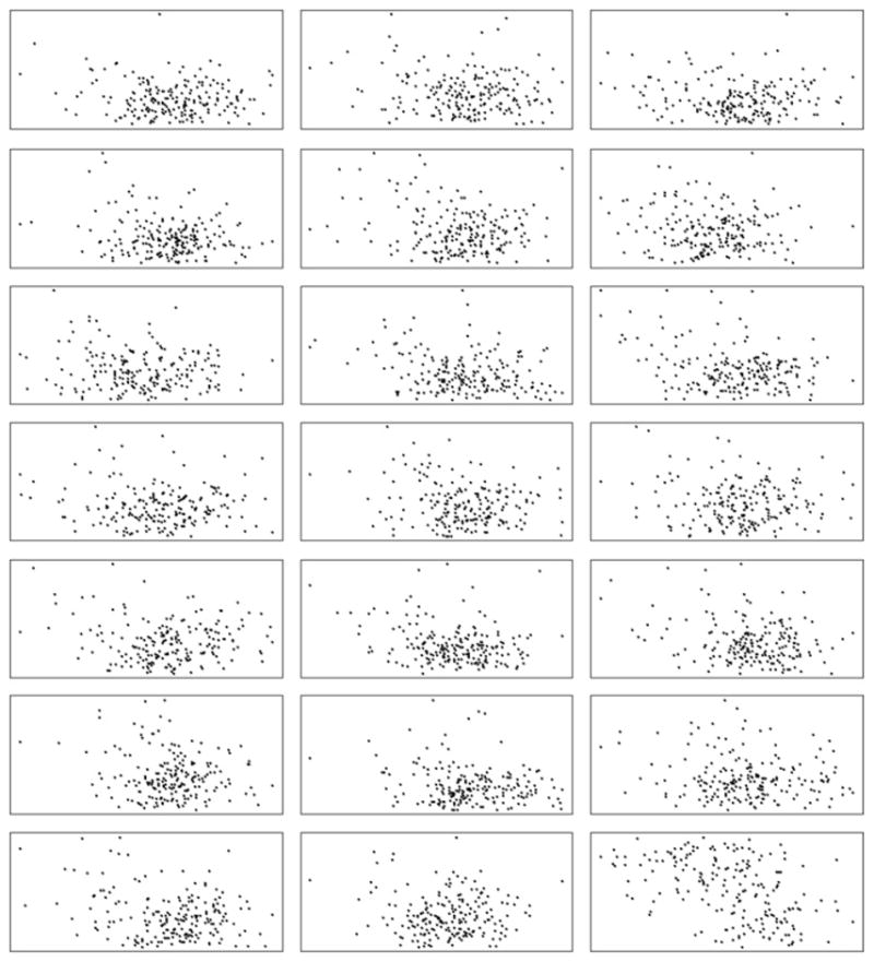
Simulated 20 datasets of 200 cases (all except the right-bottom cell) and one dataset of 200 controls (right-bottom cell).

Thus, for each dataset the total number of points is 400, among them 200 cases and 200 controls, which is the total number of points for the CL model. In the implementation of the BT model for simulated data, 200 case points and 229 dummy points (225 centroids from a 15 × 15 grid mesh plus 4 corner points) are created, giving a total of 429 points. A 20 × 20 grid mesh is considered for both the PM model and the BM model which leads to 400 cells for the mesh models. The number of dummy points in the BT model and the number of cells in the grid mesh models were chosen in such a way as to keep the total number of points close to 400.

7.1. Results

The model for the log relative risk that we have fitted by each model for simulated data is given as

$$log{\theta }_k={\beta }_0+{\beta }_1{d}_k=v_k.$$

The above model incorporates only the spatially correlated random effect, v_k, to explain all random variations in the GRF, unlike the model for real data which also include a random effect, u_k, for uncorrelated heterogeneity. It is important to note that the GRF was generated with the covariance function, cov (S_i, S_j) = 0.5 exp(−d_ij), so near zero distance the variance is expected to be close to 0.05. In other words, conditional on the model assuming an exponential covariance, if we truncate the covariance at d_ij = 0.1 then exp(−d_ij) = 0.9048. This means that cov (S_i, S_j) = 0.5 exp(−d_ij) = 0.5 approximately for small cell neighborhoods. Hence it will be true that using CAR models (which considers only the first-order neighbors) will yield a variance close to 0.5.

In order to keep consistency in choosing the prior distribution for the spatially correlated random effects, v, we adopt the conditional distribution approach for all the models and assume a CAR distribution. The prior distributions for β’s were set to normal distribution with mean 0 and large variance. In this section, we summarize the results for three parameters, the intercept β₀, the coefficient β₁, and the spatially correlated heterogeneity ${\sigma }_v^2$, which are of main interest. The parameter ρ, which is the proportion of cases to controls, was set to 1.

The boxplots in Fig. 3 display the distribution of 20 β₀’s, β₁’s and ${\sigma }_v^2$’s. The bar within the box is for the median value, the left and right ends of the box are for the first and third quartiles, and the two whiskers are for the minimum and maximum values. The mean of β₀ from the BT, CL, PM and BM models is, respectively, 2.672, 2.722, 0.337, and 2.738. For all the models the estimates of β₀ are positively biased and none of the models even includes the true value within the range. We assume it is the R function “GaussRF” responsible for these biased estimates of β₀. The current algorithm of “GaussRF” does not support generating a nonstationary GRF. By saying this we mean that a nonstationary GRF obtained by adding trend to a zero mean generated GRF, and obtained by generating a GRF with non-zero mean (i.e., trend), are not the same. In the former case (i.e., the way a nonstationary GRF was introduced in this paper), β’s connection to the spatial covariance for the generation of GRF is not well defined. We strongly believe that if the GRF were generated with nonstationary mean log (ρ) + β₀ + β₁d_i, we could have obtained better estimates of β₀.

Fig. 3.

Boxplots of β₀, β₁ and ${\sigma }_v^2$, from 20 simulated datasets where the true parameters are ${\beta }_0^{\text{true}}=-1.0,{\beta }_1^{\text{true}}=-0.005$ and ${\sigma }_v^{2,\text{true}}=0.5$. The box limits are the quartiles and whiskers are the minimum and maximum values.

The mean for β₁ from each model is respectively, −0.0044, −0.0047, −0.0024, and −0.0047. The means from the CL and BM models, and the median from the BT model for β₁, are much closer to the true value compared to the other model. The β₁ estimates from the PM model are positively biased and do not even include the true value within the range, although the estimates are very close to the true value. Similarly, the mean for ${\sigma }_v^2$ from each model is respectively, for BT, CL, PM, BM: 0.1009, 2.0509, 0.5668, and 1.7463. The mean and median values from the PM model for ${\sigma }_v^2$ are much closer to the true value compared to other models. The ${\sigma }_v^2$ estimates from the BT method and the BM model are, respectively, negatively and positively biased, and neither model even includes the true value within the range.

Table 3 gives the summary measures of error values for each model for β₀, β₁ and ${\sigma }_v^2$. For intercept β₀, the average error and the average absolute error are equal as all the models produce a positively biased estimate (Fig. 3). It is interesting to note that, among these biased estimates, the PM model has the least errors. For coefficient β₁, the CL and the BM models have the least average error and the least average absolute error. Similarly, for spatially correlated heterogeneity ${\sigma }_v^2$, the PM model has the least average error and average absolute error, and it outperforms the estimates from other models.

Table 3.

The error of the estimates over the 20 simulated datasets, where ${\beta }_0^{\text{true}}=-1.0,{\beta }_1^{\text{true}}=-0.005$, and ${\sigma }_v^{2,\text{true}}=0.5$ are the true values used in the simulation

Models	β0		β1		${\sigma }_v^2$
	$\text{Ave}\left({\widehat{\beta }}_0-{\beta }_0^{\text{true}}\right)$	$\text{Ave}\mid {\widehat{\beta }}_0-{\beta }_0^{\text{true}}\mid$	$\text{Ave}\left({\widehat{\beta }}_1-{\beta }_1^{\text{true}}\right)$	$\text{Ave}\mid {\widehat{\beta }}_1-{\beta }_1^{\text{true}}\mid$	$\text{Ave}\left({\widehat{\sigma }}_v^2-{\sigma }_v^{2,\text{true}}\right)$	$\text{Ave}\mid {\widehat{\sigma }}_v^2-{\sigma }_v^{2,\text{true}}\mid$
BT	3.67177	3.67177	0.00055	0.00056	−0.39908	0.39908
CL	3.72239	3.72239	0.00031	0.00038	1.55089	1.55089
PM	1.33660	1.33660	0.00265	0.00265	0.06677	0.06677
BM	3.73774	3.73774	0.00031	0.00038	1.24632	1.24632

8. Discussion

We compare four point process models in the assessment of the effects of a putative source of hazard (i.e., an incinerator) on the incidence of larynx cancer death in Lancashire. The BT method is a useful approximate method for analyzing point pattern health data with a normalizing integral. An important disadvantage of this method is that it is subject to quadrature error. However, this error will be insignificant for a large number of dummy points. The alternative CL model uses the exact form of likelihood rather than any form of approximation. The PM and BM models, based on the discretization of the study window, are easy to implement in any statistical packages once the binned counts are available. The “PIP” function of the R package can be used to get these counts. This paper has given a theoretical justification of these two models and illustrated the assumptions involved in that process. We also showed the equivalence between the PM model and the LGCP when discretization is preferred.

The model for log relative risks that we have considered is a multiplicative model, and it includes spatially correlated and uncorrelated random effects to explain the heterogeneity in observed data. The analysis of real data (i.e., Lancashire larynx cancer data) using the CL, PM, and BM models produces similar results. Among the discretization methods, we have observed small changes in estimates for changes in mesh size. ZIP spatial regression (Agarwal et al., 2002) can be useful for large mesh sizes, since for large mesh size many cells will have zero counts. We have also demonstrated with the PM model that a rich variety of models can be formulated based on common structured heterogeneity and/or common unstructured heterogeneity of cases and controls. This is certainly an advantage of discretization methods.

From simulated data, in estimating the intercept β₀, the average error and the average absolute error indicate that the PM model performs better compared to other models, although all the models produce positively biased estimates. We suspect that the reason for this poor performance of β₀ is the way the GRF was generated. This requires further study. In estimating the regression coefficient β₁, which is often the main interest of many epidemiological studies, the CL and BM models perform equally well. In estimating the variance parameter for spatially correlated random effects ${\sigma }_v^2$, the PM model can be singled out as the best performing model based on the least average error and the least average absolute error.

Finally, the results of simulation experiment indicate that we cannot observe a single model that performs the best in relation to every parameter of the above multiplicative model. The outcome is mixed and the choice of a specific model will depend on the study purpose. If the objective of analysis is to get estimates of coefficients, then either the CL model or BM model may be a good choice. If the interest is in explaining the heterogeneity, the PM model may be a better choice. In terms of computational time, the models based on grid meshes (BT model, PM model, and BM model) depend on the number of dummy points or number of cells. The reported results for the maximum number of cells (30 × 30) took approximately 30 min to run for 10,000 iterations in WinBUGS in a laptop with 2.33 MHz speed. The CL model took approximately the same time. Because of space limitation, we avoided providing all the WinBUGS and R codes that we have developed for this paper, but they can be made available from the first author on request.

We would also like to point out two limitations of this study. Throughout the paper we have used a CAR model for the spatially correlated random effects. Instead of this conditional specification, it is possible to adopt a multivariate normal distribution for the joint specification. We have observed that this joint distribution approach requires excessive computational time for the increased data size because at each iteration an inversion of an N × N covariance matrix will be required, where N is the number of data and dummy points in the BT method, the number of case-control events in the CL model, and the number of cells in mesh models. To circumvent this problem, resort could be made to the reduced rank kriging method (see Banerjee et al. (in press), Fuentes (2007), and Kammann and Wand (2003)). The other limitation is that we have a limited number of generated datasets for the simulation study. However, these are limited due to the computational burden of the approach.

Appendix A

Control points are generated from λ̂₀ (nonparametric estimates of intensity function for controls) as follows:

1. Set ${\widehat{\lambda }}_0=h_{{\lambda }_0}^{-1}{\sum }_{i=1}^{m}k\left(\frac{\mid \mathbf{s}-{\mathbf{s}}_i\mid }{h_{{\lambda }_0}}\right)$, where |s − s_i| is the distance between s and s_i, k(·) is an independent component bivariate kernel, and h_λ0 = (h_λ0,x, h_λ0,y)^T are the optimal smoothing parameters

2. Randomly draw a sample from set s, defined as s_sampled = (x_sampled, y_sampled)^T

3. Generate ε_x ~ N (0, 1) and ε_y ~ N (0, 1)

4. Compute x_simulate = x_sampled + h_λ0,_xε_x and y_simulate = y_sampled + h_λ0,_yε_y

5. Continue steps 2 to 4 until the desired number of control points are generated.

Appendix B

A log Gaussian Cox process has been generated for the intensity of cases, λ, as follows.

1. Generate a large number of controls for i = 1, …, m_c following the steps in Appendix A2

2. Calculate θ_i = 1 + exp(β₀ + β₁d_i), where d_i is the distance of i-th generated control point from the source

3. Generate r realizations of a Gaussian random field for S = (S₁, …, S_mc) with mean 0 and elements of the variance-covariance matrix

   $$k_{ij}(\sigma ,\alpha ,\tau )=\sigma exp(-d_{ij}/\alpha )+\tau$$

4. Calculate λ_i = ρθ_i exp(S_i)

5. Calculate λ_max = max (λ_i)

6. Randomly draw a sample from the generated controls in step 1 and define the intensity of the drawn sample as λ_sampled

7. Generate a random number, u = Uniform (0, 1)

8. If $\frac{{\lambda }_{\text{sampled}}}{{\lambda }_{max}}>u$, accept the point; otherwise, reject it. If the point is accepted, the location of this point is stored as a case location

9. Continue steps 6 to 8 until the desired number of case points are generated.

References

- Agarwal DK, Gelfand AE, Citron-Pousty S. Zero-inflated models with application to spatial count data. Environmental and Ecological Statistics. 2002;9:341–355. [Google Scholar]
- Baddeley A, Turner R. Spatstat: An R package for analyzing spatial point patterns. Journal of Statistical Software. 2005;12:1–42. [Google Scholar]
- Banerjee S, Gelfand AE, Finley AO, Sang H. Gaussian predictive process models for large spatial datasets. Journal of the Royal Statistical Society, Series B. 2008 doi: 10.1111/j.1467-9868.2008.00663.x. (in press) [DOI] [PMC free article] [PubMed] [Google Scholar]
- Berman M, Turner R. Approximating point process likelihoods with GLIM. Applied Statistics. 1992;41:31–38. [Google Scholar]
- Besag J, York J, Mollie A. Bayesian image restoration with two applications in spatial statistics (with discussion) Annals of the Institute of Statistical Mathematics. 1991;43:1–59. [Google Scholar]
- Congdon P. Applied Bayesian Models. John Wiley; 2003. [Google Scholar]
- Diggle P. Overview of statistical methods for disease mapping and its relationship to cluster detection. In: Elliott P, Wakefield J, Best N, Briggs DJ, editors. Spatial Epidemiology: Methods and Applications. Oxford University Press; 2000. [Google Scholar]
- Diggle PJ. A point process modelling approach to raised incidence of a rare phenomenon in the vicinity of a prespecified point. Journal of the Royal Statistical Society, Series A. 1990;153:349–362. [Google Scholar]
- Diggle PJ, Morris SN, Elliott P, Shaddick G. Regression modelling of disease risk in relation to point sources. Journal of the Royal Statistical Society, Series A. 1997;160:491–505. [Google Scholar]
- Diggle PJ, Rowlingson B. A conditional approach to point process modelling of elevated risk. Journal of the Royal Statistical Society, Series A. 1994;157:433–440. [Google Scholar]
- Fuentes M. Approximate likelihood for large irregularly spaced spatial data. Journal of the American Statistical Association. 2007;102:321–331. doi: 10.1198/016214506000000852. [DOI] [PMC free article] [PubMed] [Google Scholar]
- Gómez-Rubio V, Ferrándiz J, López A. In Functions for the detection of spatial clusters of diseases. 2004 http://matheron.uv.es/~virgil/Rpackages/DCluster.
- Kammann EE, Wand MP. Geoadditive models. Applied Statistics. 2003;52:1–18. [Google Scholar]
- Lawson AB. GLIM and normalising constant models in spatial and directional data analysis. Computational Statistics & Data Analysis. 1992;13:331–348. [Google Scholar]
- Lawson AB, Browne WJ, Vidal-Rodiero CL. Disease Mapping with WinBUGS and MLwiN. Wiley; New York: 2003. [Google Scholar]
- Ma B, Lawson AB, Liu Y. Evaluation of Bayesian models for focused clustering in health data. Environmetrics. 2007;18:1–16. [Google Scholar]
- Moller J, Syversveen AN, Waagepetersen RP. Log Gaussian Cox processes. Scandinavian Journal of Statistics. 1998;25:451–482. [Google Scholar]
- Okabe A, Boots B, Sugihara K, Chiu SN. Spatial Tessellations: Concepts and Applications of Voronoi Diagrams. Wiley; 2000. [Google Scholar]
- R Development Core Team. R: A language and environment for statistical computing. R Foundation for Statistical Computing; Vienna, Austria: 2004. [Google Scholar]
- Rowlingson B, Diggle P. Splancs: Spatial point pattern analysis code in S-Plus. Computers and Geosciences. 1993;19:627–655. [Google Scholar]
- Rue H, Martino S, Chopin N. Approximate Bayesian inference for latent Gaussian models using integrated nested Laplace approximations. 2007 (submitted for publication) [Google Scholar]
- Spiegelhalter D, Best N, Carlin B, Linde A. Bayesian measures of model complexity and fit (with discussion) Journal of the Royal Statistical Society, Series B. 2002;64:583–639. [Google Scholar]
- Spiegelhalter D, Thomas A, Best N, Lunn D. WinBUGS User Manual. MRC Biostatistics Unit, Institute of Public Health; Cambridge, UK: 2003. [Google Scholar]
- Waagepetersen R. Convergence of posteriors for discretized log Gaussian Cox processes. Statistics & Probability Letters. 2003;66:229–235. [Google Scholar]