Quantitative and empirical demonstration of the Matthew effect in a study of career longevity

Abstract

The Matthew effect refers to the adage written some two-thousand years ago in the Gospel of St. Matthew: “For to all those who have, more will be given.” Even two millennia later, this idiom is used by sociologists to qualitatively describe the dynamics of individual progress and the interplay between status and reward. Quantitative studies of professional careers are traditionally limited by the difficulty in measuring progress and the lack of data on individual careers. However, in some professions, there are well-defined metrics that quantify career longevity, success, and prowess, which together contribute to the overall success rating for an individual employee. Here we demonstrate testable evidence of the age-old Matthew “rich get richer” effect, wherein the longevity and past success of an individual lead to a cumulative advantage in further developing his or her career. We develop an exactly solvable stochastic career progress model that quantitatively incorporates the Matthew effect and validate our model predictions for several competitive professions. We test our model on the careers of 400,000 scientists using data from six high-impact journals and further confirm our findings by testing the model on the careers of more than 20,000 athletes in four sports leagues. Our model highlights the importance of early career development, showing that many careers are stunted by the relative disadvantage associated with inexperience.

The rate of individual progress is fundamental to career development and success. In practice, the rate of progress depends on many factors, such as an individual’s talent, productivity, reputation, as well as other external random factors. Using a stochastic model, here we find that the relatively small rate of progress at the beginning of the career plays a crucial role in the evolution of the career length. Our quantitative model describes career progression using two fundamental ingredients: (i) random forward progress “up the career ladder” and (ii) random stopping times, terminating a career. This model quantifies the “Matthew effect” by incorporating into ingredient (i) the common cumulative advantage property (1–8) that it is easier to move forward in the career the further along one is in the career. A direct result of the increasing progress rate with career position is the large disparity between the numbers of careers that are successful long tenures and the numbers of careers that are unsuccessful short stints.

Surprisingly, despite the large differences in the numbers of long and short careers, we find a scaling law that bridges the gap between the frequent short and the infrequent long careers. We test this model for both scientific and sports careers, two careers where accomplishments are methodically recorded. We analyze publication careers within six high-impact journals: Nature, Science, the Proceedings of the National Academy of Science (PNAS), Physical Review Letters (PRL), New England Journal of Medicine (NEJM), and CELL. We also analyze sports careers within four distinct leagues: Major League Baseball (MLB), Korean Professional Baseball, the National Basketball Association (NBA), and the English Premier League.

Career longevity is a fundamental metric that influences the overall legacy of an employee because for most individuals the measure of success is intrinsically related, although not perfectly correlated, to his or her career length. Common experience in most professions indicates that time is required for colleagues to gain faith in a newcomer’s abilities. Qualitatively, the acquisition of new opportunities mimics a standard positive feedback mechanism [known in various fields as Malthusian growth, cumulative advantage, preferential attachment, a reinforcement process, the ratchet effect, and the Matthew “rich get richer” effect (9)], which endows greater rewards (10) to individuals who are more accomplished than to individuals who are less accomplished.

Here we use career position as a proxy for individual accomplishment, so that the positive feedback captured by the Matthew effect is related to increasing career position. There are also other factors that result in selective bias, such as the “relative age effect,” which has been used to explain the skewed birthday distributions in populations of athletes. Several studies find that being born in optimal months provides a competitive advantage to the older group members with respect to the younger group members within a cohort, resulting in a relatively higher chance of succeeding for the older group members, consistent with the Matthew effect. This relative age effect is found at several levels of competitive sports ranging from secondary school to the professional level (11, 12).

In this paper we study the everyday topic of career longevity and reveal surprising complexity arising from the generic competition within social environments. We develop an exactly solvable stochastic model, which predicts the functional form of the probability density function (pdf) P(x) of career longevity x in competitive professions, where we define career longevity as the final career position x after a given time duration T corresponding to the termination time of the career. Our stochastic model depends on only two parameters, α and x_c. The first parameter, α, represents the power-law exponent that emerges from the pdf of career longevity. This parameter is intrinsically related to the progress rate early in the career during which professionals establish their reputations and secure future opportunities. The second parameter, x_c, is an effective time scale that distinguishes newcomers from veterans.

Quantitative Model

In this model, every employee begins his or her career with approximately zero credibility and must labor through a common development curve. At each position x in a career, there is an opportunity for progress as well as the possibility for no progress. A new opportunity, corresponding to the advancement to career position x + 1 from career position x, can refer to a day at work or, more generally, to any assignment given by an employing body. For each particular career, the change in career position Δx has an associated time frame Δt. Optimally, an individual makes progress by advancing in career position at an equal rate as the advancing of time t so that Δx ≡ Δt. However, in practice, an individual makes progress Δx in a subordinate time frame, given here as the career position x. In this framework, career progress is made at a rate that is slower than the passing of work time, representing the possibility of career stagnancy.

As a first step, we postulate that the stochastic process governing career progress is similar to a Poisson process, where progress is made at any given step with some approximate probability or rate. Each step forward in career position contributes to the employee’s resume and reputation. Hence, we refine the process to a spatial Poisson process, where the probability of progress g(x) depends explicitly on the employee’s position x within the career. In our model, the progress rate g(x) = talent(x) + reputation(x) + productivity(x) + … represents a combination of several factors, such as the talent, reputation, and productivity at a given career position x. The criteria for the Matthew effect to apply is that the progress rate be monotonically increasing with career position, so that g(x + 1) > g(x). In this paper, we do not distinguish between the Matthew effect, relating mainly to the positive feedback from recognition, and cumulative advantage, which relates to the positive feedback from both productivity and recognition (2). It would require more detailed data to determine the role of the individual factors on the evolution of a career.

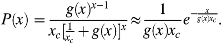
Employees begin their career at the starting career position x₀ ≡ 1 and make random forward progress through time to career position x≥1, as illustrated in Fig. 1. Career longevity is then defined as the final location x ≡ x_T along the career ladder at the time of retirement T. Let P(x|T) be the conditional probability that at stopping time T an individual is at the final career position x_T. For simplicity, we assume that the progress rate g(x) depends only on x. As a result, P(x|T) assumes the familiar Poisson form, but with the insertion of g(x) as the rate parameter,

[1]

We derive the spatial Poisson pdf P(x|T) in Appendix. In SI Appendix, we further develop an alternative model where the progress rate g(t) represents a career trajectory that depends on time (13).

Fig. 1.

Graphical illustration of the stochastic Poisson process quantifying career progress with position-dependent progress rate g(x) and stagnancy rate 1 - g(x). A new opportunity, corresponding to the advancement to career position x + 1 from career position x, can refer to a day at work or, even more generally, to any assignment given by an employing body. In this framework, career progress is made at a rate g(x) that is slower than the passing of work time, representing the possibility of career stagnancy. The traditional Poisson process corresponds to a constant progress rate g(x) ≡ λ. Here, we use a functional form for g(x) ≡ 1 - exp[-(x/x_c)^α] that is increasing with career position x, which captures the salient feature of the Matthew effect, that it becomes easier to make progress the further along the career. In SI Appendix, we further develop an alternative model where the progress rate g(t) depends on time.

According to the Matthew effect, it becomes easier for an individual to excel with increasing success and reputation. Hence, the choice of g(x) should reflect the fact that newcomers, lacking the familiarity of their peers, have a more difficult time moving forward, whereas seasoned veterans, following from their experience and reputation, often have an easier time moving forward. For this reason we choose the progress rate g(x) to have the functional form,

[2]

This function exhibits the fundamental feature of increasing from approximately zero and asymptotically approaching unity over some time interval x_c. Furthermore, g(x) ∼ x^α for small x ≪ x_c. In Fig. 2, we plot g(x) for several values of α, with fixed x_c = 10³ in arbitrary units. We will show that the parameter α is the same as the power-law exponent α in the pdf of career longevity P(x), which we plot in Fig. 2, Inset. The random process for forward progress can also be recast into the form of random waiting times, where the average waiting time 〈τ(x)〉 between successive steps is the inverse of the forward progress probability, 〈τ(x)〉 = 1/g(x).

Fig. 2.

Demonstration of the fundamental relationship between the progress rate g(x) and the career longevity pdf P(x). The progress rate g(x) represents the probability of moving forward in the career to position x + 1 from position x. The small value of g(x) for small x captures the difficulty in making progress at the beginning of a career. The progress rate increases with career position x, capturing the role of the Matthew effect. We plot five g(x) curves with fixed x_c = 10³ and different values of the parameter α. The parameter α emerges from the small-x behavior in g(x) as the power-law exponent characterizing P(x). (Inset) Probability density functions P(x) resulting from inserting g(x) with varying α into Eq. 5. The value α_c ≡ 1 separates two distinct types of longevity distributions. The distributions resulting from concave career development α < 1 exhibit monotonic statistical regularity over the entire range, with an analytic form approximated by the Gamma distribution Gamma(x; α,x_c). The distributions resulting from convex career development α > 1 exhibit bimodal behavior. In the bimodal case, one class of careers is stunted by the difficulty in making progress at the beginning of the career, analogous to a “potential” barrier. The second class of careers forges beyond the barrier and is approximately centered around the crossover x_c on a log–log scale.

We now address the fact that not every career is of the same length. Nearly every individual is faced with the constant risk of losing his or her job, possibly as the result of poor performance, bad health, economic downturn, or even a change in the business strategy of his or her employer. Survival in the workplace requires that the individual maintain his or her performance level with respect to all possible replacements. In general, career longevity is influenced by many competing random processes that contribute to the random termination time T of a career (14). Our model accounts for external termination factors that are not correlated to the contemporaneous productivity of a given individual. A more sophisticated model, which incorporates endogenous termination factors, e.g., termination due to sudden decrease in productivity below a given employment threshold, is more difficult to analytically model, which we leave as an open problem. The pdf P(x|T) calculated in Eq. 1 is the conditional probability that an individual has achieved a career position x by his or her given termination time T. Hence, to obtain an ensemble pdf of career longevity P(x), we must average over the pdf r(T) of random termination times T,

[3]

We next make a suitable choice for r(T). To this end, we introduce the hazard rate, H(T), which is the Bayesian probability that failure will occur at time T + δT, given that it has not yet occurred at time T. This is written as , where is the probability of a career surviving until time T. The exponential pdf of termination times,

[4]

has a constant hazard rate and thus assumes that external hazards are equally distributed over time. Substituting Eq. 4 into Eq. 3 and computing the integral, we obtain

[5]

Depending on the functional form of g(x), the theoretical prediction given by Eq. 5 is much different than the null model in which there is no Matthew effect, corresponding to a constant progress rate g(x) ≡ λ for each individual.

Using the functional form given by Eq. 2, we obtain a truncated power law for the case of concave α < 1, resulting in a P(x) that can be approximated by two regimes,

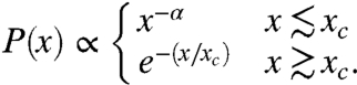[6]

Hence, our model predicts a remarkable statistical regularity that bridges the gap between very short and very long careers as a result of the concavity of g(x) in early career development.

In the case of constant progress rate g(x) ≡ λ, the pdf P(x) is exponential with a characteristic career longevity l_c = λx_c. In SI Appendix we further consider the null model where the constant progress rate λ_i of individual i is distributed over a given range. We find again that P(x) is exponential, which is quite different from the prediction given by 6. Furthermore, we also develop a second model where the progress rate depends on a generic career trajectory g(t) that peaks at a given year corresponding to the height of an individual’s talent or creativity. We solve the time-dependent model in SI Appendix for a simple form of g(t), which results in a P(x) that is peaked around the maximum career length, in contrast to our empirical findings.

In order to account for aging effects, another variation of this model could include a time-dependent H(T). To incorporate a nonconstant H(T) one can use a more general Weibull distribution for the pdf of termination times

[7]

where γ = 1 corresponds to the exponential case (15). In general, the hazard rate of the Weibull distribution is H(T) ∝ T^γ-1, where γ > 1 corresponds to an increasing hazard rate and γ < 1 corresponds to a decreasing hazard rate. We note that the time scale x_c appears both in the definition of g(x) in Eq. 2 as a crossover between early and advanced career progress rates, and also as the time scale over which the probability of survival S(T) approaches 0 in the case of γ≥1 in Eq. 4. It is the appearance of the quantity x_c in the definition of S(T) that results in a finite exponential cutoff to the longevity distributions. Although the time scales defined in g(x) and S(T) could be different, we observe only one time scale in the empirical data. Hence we assume here for simplicity that the two time scales are approximately equal.

From the theoretical curves plotted in Fig. 2, Inset, one observes that α_c = 1 is a special crossover value for P(x), between a bimodal P(x) for α > 1, and a monotonically decreasing P(x) for α < 1. This crossover is due to the small x behavior of the progress rate g(x) ≈ x^α for x < x_c, which serves as a “potential barrier” that a young career must overcome. The width x_w of the potential barrier, defined such that g(x_w) = 1/x_c, scales as . Hence, the value α_c = 1 separates convex progress (α > 1) from concave progress (α < 1) in early career development.

In the case α > 1, one class of careers is stunted by the barrier, whereas the other class of careers excels, resulting in a bimodal P(x). In the case α < 1, it is relatively easier to make progress in the beginning of the career. It has been shown in ref. 16 that random stopping times can explain power-law pdfs in many stochastic systems that arise in the natural and social sciences, with predicted exponent values α≥1. Our model provides a mechanism that predicts truncated power-law pdfs with scaling exponents α ≤ 1, where the truncation is a requirement of normalization. Moreover, our model provides a quantitative meaning for the power-law exponent α characterizing the probability density function.

Empirical Evidence

The two essential ingredients of our stochastic model, namely random forward progress and random termination times corresponding to a stochastic hazard rate, are general and should apply in principle to many competitive professions. The individuals, some who are championed as legends and stars, are judged by their performances, usually on the basis of measurable metrics for longevity, success, and prowess, which vary between professions.

In scientific arenas, and in general, the metric for career position is difficult to define, even though there are many conceivable metrics for career longevity and success (17–19). We compare author longevity within individual journals, which mimic an arena for competition, each with established review standards that are related to the journal prestige. As a first approximation, the career longevity of a given author within a particular high-impact journal can be roughly measured as the duration between an author’s first and last paper in that journal, reflecting his or her ability to produce at the top tiers of science. This metric for longevity should not be confused with the career length of the scientist, which is probably longer than the career longevity within any particular journal. Following standard lifetime data analysis methods (20), we collect “completed” careers from our dataset. The publication data we collect for each journal begins at year Y₀ = 1958 for all journals except for CELL (for which Y₀ = 1974), and ends at year Y_f = 2008.

For each scientific career i, we calculate 〈Δτ_i〉, the average time between publications in a particular journal. A journal career that begins with a publication in year y_i,0 and ends with a publication in year y_i,f is considered “complete” if the following two criteria are met: (I) y_i,f ≤ Y_f - 〈Δτ_i〉 and (ii) y_i,0≥Y₀ + 〈Δτ_i〉. These criteria help eliminate from our analysis incomplete careers that possibly began before Y₀ or ended after Y_f. We then estimate the career length within journal j as L_i,j = y_i,f - y_i,0 + 1, with a year allotted for publication time, and do not consider careers with y_i,f = y_i,0. This reduces the size of each journal dataset by approximately 25% (for a description of data and methods, see SI Appendix (Sec. I and Table S1)).

In ref. 21 we further analyze the scientific careers of the authors in these six journal databases. In order to account for time-dependent and discipline-dependent factors that affect both success and productivity measures, we develop normalized metrics for career success (“citation shares”) and productivity (“papers shares”). We also find further evidence of the Matthew effect by analyzing the interpublication time τ(x) that decreases with increasing publication x for individual authors within a given journal. Thus, we conclude that publication in a particular journal is facilitated by previous publications in the journal, corresponding to an increasing reputation within the given journal (22). Several other metrics for quantifying career success (18, 23), such as the h index (17) and generalizations (24, 25), along with methods for removing time- and discipline-dependent citation factors (26) have been analyzed in the spirit of developing unbiased rating systems for scientific achievement.

In athletic arenas, the metrics for career position, success, and success rate are easier to define (27). In general, a career position in sports can be measured by the cumulative number of in-game opportunities a player has obtained. In baseball, we define an opportunity as an “at bat” (AB) for batters and an “inning pitched in outs” (IPO) for pitchers, whereas in basketball and soccer, we define the metrics for opportunity as “minutes played” and “games played,” respectively.

In Fig. 3 we plot the distributions of career longevity for 20,000 professional athletes in four distinct leagues and roughly 400,000 scientific careers in six distinct journals (data are publicly available at refs. 28 and 29). We observe universal statistical regularity corresponding to α < 1 in the career longevity distributions for three distinct sports and several high-impact journals (see Table S2 for a summary of least squares parameters). The disparity in career lengths indicates that it is very difficult to sustain a competitive professional career, with most individuals making their debut and finale over a relatively short time interval. For instance, we find that roughly 3% of baseball pitchers have a career length in the MLB of one inning pitched or less, whereas we also find that roughly 3% of basketball players have a career length in the NBA of less than 12 in-game minutes. Yet, despite the relatively high frequency of short careers, there are also instances of careers that are extremely long, corresponding to roughly the entire productive lifetime of the individual. The statistical regularity that bridges the gap between the “one-hit wonders” and the “iron horses” indicates that there are careers of every length between the minimum and the maximum career length, with a smooth and monotonic relation quantifying the relative frequencies of the careers in between. Furthermore, we find that stellar careers are not anomalies, but rather, as predicted by our model, the outcome of the cumulative advantage in competitive professions. The properties of the cumulative advantage process are also compounded by an individual’s “sacred spark” factor (2) that accounts for his or her relative level of talent and/or professional drive, which also factors into career longevity.

Fig. 3.

Extremely right-skewed pdfs P(x) of career longevity in several high-impact scientific journals and several major sports leagues. We analyze data from American baseball (Major League Baseball) over the 84-year period 1920–2004, Korean Baseball (Korean Professional Baseball League) over the 25-year period 1982–2007, American basketball (National Basketball Association and American Basketball Association) over the 56-year period 1946–2004, and English soccer (Premier League) over the 15-year period 1992–2007, and several scientific journals over the 42-year period 1958–2000. Solid curves represent least-squares best-fit functions corresponding to the functional form in Eq. 5. (A) Baseball fielder longevity measured in at-bats (pitchers excluded): we find α ≈ 0.77, x_c ≈ 2,500 (Korea) and x_c ≈ 5,000 (United States). (B) Basketball longevity measured in minutes played: we find α ≈ 0.63, x_c ≈ 21,000 minutes. (C) Baseball pitcher longevity measured in IPO: we find α ≈ 0.71, x_c ≈ 2,800 (Korea), and x_c ≈ 3,400 (United States). (D) Soccer longevity measured in games played: we find α ≈ 0.55, x_c ≈ 140 games. (E and F) High-impact journals exhibit similar longevity distributions for the “journal career length,” which we define as the duration between an author’s first and last paper in a particular journal. Deviations occur for long careers due to dataset limitations (for comparison, least-square fits are plotted in E with parameters α ≈ 0.40, x_c = 9 years and in F with parameters α ≈ 0.10, x_c = 11 years). These statistics are summarized in SI Appendix (Table S2).

The exponential cutoff in P(x) that follows after the crossover value x_c arises from the finite human lifetime and is reminiscent of any real system where there are finite-size effects that dominate the asymptotic behavior. The scaling regime is less pronounced in the curves for journal longevity. This results from the granularity of our dataset, which records publications by year only. A finer time resolution (e.g., months between first and last publication) would likely reveal a larger scaling regime. However, regardless of the scale, one observes the salient feature of there being a large disparity between the frequency of long and short careers.

In science, an author’s success metric can be quantified by the total number of papers or citations in a particular journal. Publication careers have the important property that the impact of scientific work is time dependent. Where many papers become outdated as the scientific body of knowledge grows, there are instances where “late-blooming” papers make significant impact a considerable time after publication (30). Accounting for the time-dependent properties of citation counts, in ref. 21 we find that the pdf of total number of normalized citation shares for a particular author in a single journal over his or her entire career follows the asymptotic power law P(z)dz ∼ z^-2.5dz for the six journals analyzed here.

In sports, however, career accomplishments do not wax or wane with time. In Fig. 4 we plot the pdf P(z) of career success z for common metrics in baseball and basketball. Remarkably, the power-law regime for P(z) is governed by a scaling exponent that is approximately equal to the scaling exponent of the longevity pdf P(x). In SI Appendix, we show that the pdf P(z) of career success z follows directly from a simple Mellin convolution of the pdf P(x) for longevity x and the pdf P(y) of prowess y.

Fig. 4.

Probability density function P(z) of common metrics for career success, z. Solid curves represent best-fit functions corresponding to Eq. 5. (A) Career batting statistics in American baseball: , , (RBI = runs batted in). (B) Career statistics in American basketball: , . For clarity, the top set of data in each plot has been multiplied by a constant factor of four in order to separate overlapping data.

The Gamma pdf P(x) = Gamma(x; α,x_c) ∝ x^-αe^-x/x_c is commonly employed in statistical modeling and can be used as an approximate form of 6. One advantage to the Gamma pdf is that it can be inverted in order to study extreme statistics corresponding to rare stellar careers. In SI Appendix and in ref. 31, we further analyze the relationship between the extreme statistics of the Gamma pdf and the selection processes for Hall of Fame museums. In general, the statistical regularity of these distributions allows one to establish robust milestones, which could be used for setting the corresponding financial rewards and pay scales, within a particular profession. Interestingly, we also find in ref. 31 that the pdfs for career success in MLB are stationary even if we quantitatively remove the time-dependent factors that can relatively inflate or deflate measures for success. This stationarity implies that the right-skewed statistical regularity we observe in P(z) arises from both the intrinsic talent and the longevity of professional athletes and does not result from changes in technology, economic factors, training improvements, etc. In the case of MLB, this detrending method allows one to compare the accomplishments of baseball players across historical eras and, in particular, can help to interpret and quantify the relative achievements of players from the recent “steroids era.”

In summary, a wealth of data recording various facets of social phenomena has become available in recent years, allowing scientists to search for universal laws that emerge from human interactions (32). Theoretical models of social dynamics, employing methods from statistical physics, have provided significant insight into the various mechanisms that can lead to emergent phenomena (33). An important lesson from complex system theory is that oftentimes the details of the underlying mechanism do not affect the macroscopic emergent phenomena. For baseball players in Korea and the United States, we observe remarkable similarity between the pdfs of career longevity (Fig. 3) and the pdfs of prowess (Fig. S1), despite these players belonging to completely distinct leagues. This fact is consistent with the hypothesis that universal stochastic forces govern career development in science, professional sports, and presumably in a large class of competitive professions.

In this paper we demonstrate strong empirical evidence for universal statistical laws that describe career progress in competitive professions. Universal phenomena also occur in many other social complex systems where regularities arise despite the complexity of the human interactions and the spatiotemporal dynamics (34–47). Stemming from the simplicity of the assumptions, the stochastic model developed in this paper could conceivably apply elsewhere in society, such as the duration of both platonic and romantic friendships. Indeed, long relationships are harder to break than short ones, with random factors inevitably terminating them forever. Also, supporting evidence for the applicability of this model can be found in the similar truncated power-law pdfs with α < 1, which describe the dynamics of connecting within online social networks (43).

Appendix: The Spatial Poisson Distribution

The master equation for the evolution of P(x,N) is

[8]

with initial condition

[9]

Here f(x) represents the probability that an employee obtains another future opportunity given his or her resume at career position x. We next write the discrete-time discrete-space master equation in the continuous-time discrete-space form

[10]

where g(x) = f(x)/δt and t = Nδt (for an extensive discussion of master equation formalism, see ref. 48). Taking the Laplace transform of both sides, one obtains

[11]

From the initial condition in Eq. 9, we see that the second term above vanishes for x≥1. Solving for P(x + 1,s) we obtain the recurrence equation

[12]

If the first derivative is relatively small, we can replace g(x + 1) with g(x) in the equation above. Then, one can verify the ansatz

[13]

which is the Laplace transform of the spatial Poisson distribution P[x,t; λ = g(x)] as in ref. 49. The Laplace transform is defined as . Inverting the transform we obtain

[14]

Hence, Eq. 14 corresponds to the pdf of final career position x observed at a particular time t. Because not all careers last the same length of time, we define the time t ≡ T to be a conditional stopping time that characterizes a given subset of careers that lasted a time duration T. We average over a distribution r(T) of stopping times to obtain the empirical longevity pdf P(x) in Eq. 5, which is equivalent to Eq. 13, so that P(x) is comprised of careers with varying T.

References

- 1.Merton RK. The Matthew effect in science. Science. 1968;159:56–63. [PubMed] [Google Scholar]
- 2.Allison PD, Stewart JA. Productivity differences among scientists: Evidence for accumulative advantage. Am Sociol Rev. 1974;39:596–606. [Google Scholar]
- 3.De Solla Price D. A general theory of bibliometric and other cumulative advantage processes. J Am Soc Inf Sci. 1976;27:292–306. [Google Scholar]
- 4.Allison PD, Long SL, Krauze TK. Cumulative advantage and inequality in science. Am Sociol Rev. 1982;47:615–625. [Google Scholar]
- 5.Merton RK. The Matthew effect in science, II: Cumulative advantage and the symbolism of intellectual property. ISIS. 1988;79:606–623. [Google Scholar]
- 6.Walberg JH, Tsai S. Matthew effects in education. Am Educ Res J. 1983;20:359–373. [Google Scholar]
- 7.Stanovich KE. Matthew effects in reading: Some consequences of individual differences in the acquisition of literacy. Read Res Quart. 1986;21:360–407. [Google Scholar]
- 8.Bonitz M, Bruckner E, Scharnhorst A. Characteristics and impact of the Matthew effect for countries. Scientometrics. 1997;40:407–422. [Google Scholar]
- 9. “For to all those who have, more will be given, and they will have an abundance; but from those who have nothing, even what they have will be taken away.” Matthew 25:29, New Revised Standard Version.
- 10.Cole S, Cole JR. Scientific output and recognition: A study in the operation of the reward system in science. Am Sociol Rev. 1967;32:377–390. [PubMed] [Google Scholar]
- 11.Helsen WF, Starkes JL, Van Winckel J. The influence of relative age on success and dropout in male soccer players. Am J Hum Biol. 1998;10:791–798. doi: 10.1002/(SICI)1520-6300(1998)10:6<791::AID-AJHB10>3.0.CO;2-1. [DOI] [PubMed] [Google Scholar]
- 12.Musch J, Grondin S. Unequal competition as an impediment to personal development: A review of the relative age effect in sport. Dev Rev. 2001;21:147–167. [Google Scholar]
- 13.Simonton DK. Creative productivity: A predictive and explanatory model of career trajectories and landmarks. Psychol Rev. 1997;104:66–89. [Google Scholar]
- 14.Segalla M, Jacobs-Belschak G, Müller C. Cultural influences on employee termination decisions: Firing the Good, Average or the Old? Eur Manag J. 2001;19:58–72. [Google Scholar]
- 15.Lawless JF. Statistical Models and Methods for Lifetime Data. 2nd Ed. New York: Wiley; 2003. [Google Scholar]
- 16.Reed WJ, Hughes BD. From gene families and genera to incomes and internet file sizes: Why power laws are so common in nature. Phys Rev E. 2002;66:067103. doi: 10.1103/PhysRevE.66.067103. [DOI] [PubMed] [Google Scholar]
- 17.Hirsch JE. An index to quantify an individual’s scientific research output. Proc Natl Acad Sci USA. 2005;102:16569–16572. doi: 10.1073/pnas.0507655102. [DOI] [PMC free article] [PubMed] [Google Scholar]
- 18.Radicchi F, Fortunato S, Markines B, Vespignani A. Diffusion of scientific credits and the ranking of scientists. Phys Rev E. 2009;80:056103. doi: 10.1103/PhysRevE.80.056103. [DOI] [PubMed] [Google Scholar]
- 19.Davies JA. The individual success of musicians, like that of physicists, follows a stretched exponential distribution. Eur Phys J B. 2002;27:445–447. 10.1140/epjb/ e2002-00176-y. [Google Scholar]
- 20.Huber JC. Inventive productivity and the statistics of exceedances. Scientometrics. 1999;45:33–53. [Google Scholar]
- 21.Petersen AM, Wang F, Stanley HE. Methods for measuring the citations and productivity of scientists across time and discipline. Phys Rev E. 2010;81:036114. doi: 10.1103/PhysRevE.81.036114. [DOI] [PubMed] [Google Scholar]
- 22.Castillo C, Donato D, Gionis A. Estimating Number of Citations Using Author Reputation. Berlin: Springer; 2007. (Lecture Notes in Computer Science). [Google Scholar]
- 23.Sidiropoulos A, Manolopoulos Y. Generalized comparison of graph-based ranking algorithms for publications and authors. J Syst Software. 2006;79:1679–1700. [Google Scholar]
- 24.Sidiropoulos A, Katsaros D, Manolopoulos Y. Generalized Hirsch h-index for disclosing latent facts in citation networks. Scientometrics. 2007;72:253–280. [Google Scholar]
- 25.Batista PD, Campiteli MG, Martinez AS. Is it possible to compare researchers with different scientific interests? Scientometrics. 2006;68:179–189. [Google Scholar]
- 26.Radicchi F, Fortunato S, Castellano C. Universality of citation distributions: Toward an objective measure of scientific impact. Proc Natl Acad Sci USA. 2008;105:17268–17272. doi: 10.1073/pnas.0806977105. [DOI] [PMC free article] [PubMed] [Google Scholar]
- 27.Petersen AM, Jung W-S, Stanley HE. On the distribution of career longevity and the evolution of home-run prowess in professional baseball. Europhys Lett. 2008;83:50010. [Google Scholar]
- 28. Sean Lahman’s Baseball Archive: http://baseball1.com/index.php; Korean Professional Baseball League: http://www.inning.co.kr; Database Sports Basketball Archive: http://www.databasebasketball.com/; Barclays Premier League: http://www.premierleague.com/
- 29. ISI Web of Knowledge: www.isiknowledge.com/
- 30.Redner S. Citation statistics from 110 years of Physical Review. Phys Today. 2005;58(6):49–54. [Google Scholar]
- 31.Petersen AM, Penner O, Stanley HE. Methods for detrending success metrics to account for inflationary and deflationary factors. Eur Phys J B. 2010 10.1140/epjb/e2010-10647-1. [Google Scholar]
- 32.Lazer D, et al. Computational social science. Science. 2009;323:721–723. doi: 10.1126/science.1167742. [DOI] [PMC free article] [PubMed] [Google Scholar]
- 33.Castellano C, Fortunato S, Loreto V. Statistical physics of social dynamics. Rev Mod Phys. 2009;81:591–646. [Google Scholar]
- 34.Liljeros F, et al. The web of human sexual contacts. Nature. 2001;411:907–908. doi: 10.1038/35082140. [DOI] [PubMed] [Google Scholar]
- 35.de Blasio BF, Svensson A, Liljeros F. Preferential attachment in sexual networks. Proc Natl Acad Sci USA. 2007;104:10762–10767. doi: 10.1073/pnas.0611337104. [DOI] [PMC free article] [PubMed] [Google Scholar]
- 36.Newman MEJ. Power laws, Pareto distributions and Zipf’s law. Contemp Phys. 2005;46:323–351. [Google Scholar]
- 37.Farmer JD, Shubik M, Smith E. Is economics the next physical science? Phys Today. 2005;58(9):37–42. [Google Scholar]
- 38.Barabási AL. The origin of bursts and heavy tails in human dynamics. Nature. 2005;435:207–211. doi: 10.1038/nature03459. [DOI] [PubMed] [Google Scholar]
- 39.Watts DJ, Strogatz SH. Collective dynamics of small-world networks. Nature. 1998;393:440–442. doi: 10.1038/30918. [DOI] [PubMed] [Google Scholar]
- 40.González MC, Hidalgo CA, Barabási AL. Understanding individual human mobility patterns. Nature. 2008;453:779–782. doi: 10.1038/nature06958. [DOI] [PubMed] [Google Scholar]
- 41.Malmgren RD, et al. A Poissonian explanation for heavy tails in e-mail communication. Proc Natl Acad Sci USA. 2008;105:18153–18158. doi: 10.1073/pnas.0800332105. [DOI] [PMC free article] [PubMed] [Google Scholar]
- 42.Crane R, Sornette D. Robust dynamic classes revealed by measuring the response function of a social system. Proc Natl Acad Sci USA. 2008;105:15649–15653. doi: 10.1073/pnas.0803685105. [DOI] [PMC free article] [PubMed] [Google Scholar]
- 43.Leskovec J, et al. Microscopic evolution of social networks; Proceedings of the ACM SIGKDD International Conference on Knowledge Discovery and Data Mining, KDD’08; New York: Association for Computing Machinery; 2008. pp. 462–470. [Google Scholar]
- 44.Petersen AM, Wang F, Havlin S, Stanley HE. Quantitative law describing market dynamics before and after interest rate change. Phys Rev E. 2010;81:066121. doi: 10.1103/PhysRevE.81.066121. [DOI] [PubMed] [Google Scholar]
- 45.Jung W-S, Wang F, Stanley HE. Gravity model in the Korean highway. Europhys Lett. 2008;81:48005. [Google Scholar]
- 46.Lee K, Jung W-S, Park JS, Choi MY. Statistical analysis of the Metropolitan Seoul Subway System: Network structure and passenger flows. Physica A. 2008;387:6231–6234. [Google Scholar]
- 47.Song C, Koren T, Wang P, Barabási AL. Modeling the scaling properties of human mobility. Nat Phys. 2010;6:818–823. [Google Scholar]
- 48.Redner S. A Guide to First-Passage Processes. Cambridge, UK: Cambridge Univ Press; 2001. [Google Scholar]
- 49.Larson RC, Odoni AR. Urban Operations Research. 2nd Ed. Charlestown, MA: Dynamic Ideas; 2007. [Google Scholar]
Associated Data
This section collects any data citations, data availability statements, or supplementary materials included in this article.