Visualization of the protein-coding regions with a self adaptive spectral rotation approach

Abstract

Identifying protein-coding regions in DNA sequences is an active issue in computational biology. In this study, we present a self adaptive spectral rotation (SASR) approach, which visualizes coding regions in DNA sequences, based on investigation of the Triplet Periodicity property, without any preceding training process. It is proposed to help with the rough coding regions prediction when there is no extra information for the training required by other outstanding methods. In this approach, at each position in the DNA sequence, a Fourier spectrum is calculated from the posterior subsequence. Following the spectrums, a random walk in complex plane is generated as the SASR's graphic output. Applications of the SASR on real DNA data show that patterns in the graphic output reveal locations of the coding regions and the frame shifts between them: arcs indicate coding regions, stable points indicate non-coding regions and corners’ shapes reveal frame shifts. Tests on genomic data set from Saccharomyces Cerevisiae reveal that the graphic patterns for coding and non-coding regions differ to a great extent, so that the coding regions can be visually distinguished. Meanwhile, a time cost test shows that the SASR can be easily implemented with the computational complexity of O(N).

INTRODUCTION

It is well known that a significant function of DNA is to instruct the synthesis of the proteins, which are basic organic compounds made of amino acids arranged in a linear chain. Detecting the protein-coding regions in the DNA sequence has become an active issue in the field of computational biology (1–10). The hidden Markov model (HMM) based methods are most developed techniques for this issue (11–14). They predict the coding regions with extreme high accuracy, after the models are trained by suitable training sets. However, the training dependence may reduce adaptability of the methods, particularly for new sequences from unknown organism with no or small training sets (11). Therefore, it is significant to predict, even roughly, locations of the coding regions without training process, before any extra information can be used. In this work, we developed an approach to visualize the coding regions by investigating a coding related property, i.e. the Triplet Periodicity (TP) property, so that the rough locations of the coding regions can be pointed out manually or computationally.

In the protein-coding regions, 20 different kinds of amino acids are coded by triplets of DNA residues, which are known as codons. Researchers suggest that the usages of codons are highly non-random in the coding regions (15). The biased appearance of codons raises a universal property in the coding regions, called the ‘TP’. Investigating the TP property can be a subject of interest for developing the coding regions detection algorithm (16,17), as well as some other significant gene related issues. The TP property was first presented by Fickett (18). It is said to be a simple and universal difference between coding and non-coding regions. After Fickett’s work, the TP property was analyzed concerning various theoretical tools, such as the hidden Markov chains (19,20), the time series (21,22), the information theory (15,16) and the Fourier transform (23–29). Using the Fourier transform, Tiwari et al. (23) developed a measure, known as Spectral Content Measure (SCM) to investigate the intensity of TP and further construct a gene predictor. A family of methods have grown from the original SCM, since researchers extended and improved Tiwari’s original method in many ways (27–38). Among these methods, Anastassiou’s (27,28) Optimized Spectral Content Measure (OSCM) and Kotlar and Lavner’s (29) Spectral Rotation Measure (SRM) are said to be distinctive. They consider not only the intensity of the TP property, but also the fact that the TP property in the coding regions varies from a certain organism to another, each organism may have its specific TP profile. In OSCM and SRM, the specific TP profile for the target organism is presented in different mathematical forms, i.e. the four coefficients in OSCM (27) and the phase angles’ expected values and variances in SRM (29). A ‘profile matching’ (see details in the ‘Materials and Methods’ section), rather than considering only the intensity of TP, makes the measures more powerful.

However, there are still some significant concerns. Most of the TP based methods with high performance, such as OSCM and SRM, need the known genes’ data from the target organism, or its close relations, for training. They are also training dependent, like the HMM based methods, and it limits the application of these methods on the unknown organisms, which cannot provide sufficient known gene data for training. Moreover, most of the SCM related methods are ‘measure-based’. In order to detect the TP property and further find the potential coding regions in the large DNA sequence, they employ moving slide windows to investigate their measures in local sections of the sequence (23,27,29). The sensitivity of these methods highly depends on the length of the slide window. A fixed length 351 bp has been used in Tiwari et al.’s work (23), Anastassiou’s work (27) and Kotlar and Lavner’s work (29). However, there is always a trade-off in selecting a fixed window’s length or an analysis scale (29), since the fixed scale is not always suitable in all situations.

In this article, a new approach named self adaptive spectral rotation (SASR) is proposed to visualize the coding regions in the DNA sequence. A hidden TP profile is automatically maintained in the SASR. So it is not necessary to carry out any training, and the powerful ‘profile matching’ can be applied to the new and unknown organisms, by using the SASR. Meanwhile, without using the fixed slide window or analysis scale, the SASR obtains a graphic output, called the TP walk, which visually reveals the locations of the coding regions and the frame shifts between them. The paper is organized as follows: In the ‘Materials and Methods’ section, we first review some coding region identification methods, which are based on the TP property and the Fourier transform. Then the newly proposed SASR approach is presented in detail. The ‘Results’ section shows some applications of the SASR on real DNA data sets. The practical output of the SASR is discussed, to investigate the principle of the graphic output for visualizing the TP property. The applications on genomic data sets from Saccharomyces Cerevisiae reveal the high capability of the SASR's output, in discriminating coding and non-coding regions. The ‘Discussion’ section compares the SASR with some other methods, indicating its advantages and significant features.

MATERIALS AND METHODS

The DNA sequences’ data set

The DNA sequence data involved in this work were collected from NCBIs Entrez Nucleotide database (http://www.ncbi.nlm.nih.gov/sites/entrez?db=nucleotide), which is a combined source database, including GenBank, RefSeq, TPA and PDB. The mitochondrial DNA sequences from Homo sapiens (Human), Gallus gallus (Chicken) and Halichoerus grypus (Gray Seal) were collected on 18 March 2009, and the S. cerevisiae chromosome sequences were collected on 12 August 2009. Fragments and complete sequences of the mitochondrial DNA were used to investigate the practical behavior of the SASR's output in various cases. In the capability evaluations, the single-exon genes with ‘experimental evidence’ from the first 15 chromosomes of S. cerevisiae were extracted as the positive sample set and the inner sequences between genes from these chromosomes were extracted as the negative sample set. The single-exon genes, which are with ‘experimental evidence’ and in the forward reading direction, from the 16th chromosome of S. cerevisiae were extracted as the training set to obtain the coefficients used in the SRM.

Identifying coding regions based on the TP property, with the Fourier transform

In Tiwari et al.’s work (23), a DNA sequence was represented as four binary sequences of the Voss model (39), i.e. u_A(t), u_T(t), u_G(t) and u_C(t) for t = 1, 2, 3, … , N. N stands for the length of the sequence. u_Λ(t) = 1 if and only if the nucleotide base Λ (Λ = A, T, C or G) appears at the position t. Consider the Fourier Transform on the four sequences, which is:

Four complex spectrums can be obtained at frequency f = N/3, i.e. U_A(N/3), U_T(N/3), U_G(N/3) and U_C(N/3). The SCM is the square sum of these four components:

The measure is said to be the same as the sum of the four position asymmetry measures (up to a 3/2 multiplicative factor) (29), which were proposed by Fickett and Tung (40). A high value of SCM suggests a high intensity of TP, and further reveals a coding region.

In 2000, Anastassiou introduced the OSCM by assigning four optimized weights to the four complex components (27,28):

The weights a, t, g and c are obtained by training on the known genes from the target organism, in order to optimize the prediction specifically for this organism. It has been reported that the OSCM is more significant than the original SCM for predicting genes in S. cerevisiae (27).

Kotlar and Lavner (29) further proposed a SRM by considering the statistical property of the four complex components’ arguments, i.e. arg[U_A(N/3)], arg[U_T(N/3)], arg[U_G(N/3)] and arg[U_C(N/3)]. They suggested that, in coding regions from a given organism, the TP property implies a bell-shaped distribution of each component’s argument, i.e. arg[U_Λ(N/3)], and the distribution is close to uniform in the non-coding regions without the TP property. Hence, in the coding regions, the four components can be rotated to a same direction by four multiplications:

μ_Λ is the expected value of arg[U_Λ(N/3)] obtained from the known genes of the target organism. Then the SRM is defined by the rotated components:

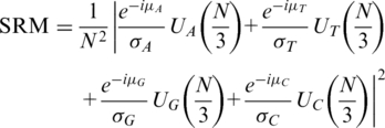Here, σ_Λ stands for the variance of arg[U_Λ(N/3)], also obtained from the known genes, and it is used in the measure to give more weights to narrower distributions (29). A high value of SRM reveals a coding region, since only in the coding regions can the four components be rotated to a same direction and produce a high summation. Kotlar and Lavner (29) suggested that considering the arguments of the Fourier spectra yields more information than the corresponding magnitudes alone.

Introducing the TP vector

The TP profile was presented in Frenkel and Korotkov’s work (15) using a Triplet Periodicity Matrix (TPM). The TPM is a 4 × 3 matrix, each row i (i = 1, 2, 3, 4) stands for a nucleotide base (A, T, C or G), each column stands for a position j (j = 1, 2, 3) in the period and the entry m_ij is the count by which the base i appears at the position j. Here, we also consider the TPM as a representation of the TP profile.

Considering the Tiwari’s method (23), the Fourier spectrum at N/3 for the base Λ (Λ = A, T, C or G) is:

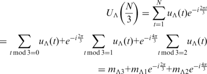(1)

For each nucleotide base Λ, the triplet row vector M = {m_Λ1, m_Λ2, m_Λ3} from Frenkel and Korotkov’s TPM is an equivalence of the Fourier spectrum U_Λ(N/3). In this work, this triplet row vector M is called a TP vector and its corresponding Fourier spectrum is considered as its complex form. The TP vector of a given DNA sequence X for the nucleotide base Λ is then denoted here in a function form: M_Λ(X).

Here, we define two cyclic shifts, i.e. left cyclic shift (LCS) and right cyclic shift (RCS), on the TP vector. The shift operations are to shift the values among the three elements. An LCS shifts the original TP vector {m₁, m₂, m₃} into {m₂, m₃, m₁}, and an RCS shifts the vector into {m₃, m₁, m₂}. The shift operations are denoted by two symbols ‘<<’ and ‘>>’: M << k stands for k times LCS on M, and M >> k stands for k times RCS. According to Equation 1, it is easy to find that a 2πk/3 counter clockwise rotation on the Fourier spectrum can be easily implemented by k times LCS on its corresponding TP vector M, i.e. M << k, while M >> k is equivalent to a 2πk/3 clockwise rotation. It is also noticed that, the addition, subtraction and multiplication on a TP vector M are equivalent to the same operations on its corresponding Fourier spectrum U, i.e. M ± M′ ↔ U ± U′ and cM ↔ cU (c is a real number). Besides, the length of a TP vector L(M) is defined here as the norm of its corresponding Fourier spectrum, i.e. L(M) = |U|.

The SASR

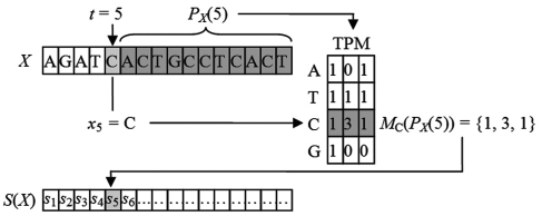
The SASR starts with a transformation from the DNA sequence to a TP vector’s sequence, named TP sequence. Consider a given DNA sequence, which is a sequence of nucleotide bases X = {x_t | t = 1, 2, 3 … , N}. The posterior subsequence of X at position t₀ is denoted as P_X(t₀) = {x_t | t₀ < t ≤ N}. The TP sequence, transformed from X, is defined as a sequence of TP vectors S(X) = {s_t | t = 1, 2, 3, … , N}, obtained as: s_t = Mx_t(P_X(t)). That is for each position t, calculate the TP vector s_t of the posterior subsequence P_X(t) for the nucleotide base x_t. Figure 1 shows an example explaining the transformation from the DNA sequence to the TP sequence.

Figure 1.

Transforming the DNA sequence into the TP sequence.

According to this description of the TP sequence, for each position t, the posterior subsequence is considered and a TP vector is calculated. It reveals that, in practice, generating a TP sequence from a DNA sequence is time consuming with the computational complexity of O(N²). In order to reduce the computational complexity, a recursive algorithm is developed here.

It is noticed that P_X(t+1) is a posterior subsequence of P_X(t). Then the algorithm is to recursively calculate M_Λ(P_X(t)) from M_Λ(P_X(t+1)), with the recurrence equation:

(2)

The recursive process is with the initial value M_Λ(P_X(N)) = {0, 0, 0}. Hence, M_Λ(P_X(t)) can be calculated recursively from the 3′- to 5′-end. In other words, we maintain a TPM of the posterior subsequence from position N to 1. Consequently, the TP sequence can be generated by choosing s_t, at each position t, from the four vectors, i.e. M_A(P_X(t)), M_T(P_X(t)), M_C(P_X(t)) and M_G(P_X(t)). The algorithm is described in the pseudo code as below.

TP sequence generation algorithm
Input: DNA sequence x[1 … N]
Output: TP sequence s[1 … N]
1	For each Λ do M[Λ] = {0, 0, 0};
2	t = N;
3	While(t>0) do{
4	s[t] = M[x[t]];
5	For each Λ do{
6	M[Λ] = M[Λ] >> 1;
7	If(x[t]==Λ) M[Λ] = M[Λ] + {1, 0, 0};
8	}
9	t––;
10	}

An example is given in Figure 2. Obviously, the computational complexity is reduced to O(N) by using this algorithm.

Figure 2.

The TP sequence generation algorithm.

After the transformation from the DNA sequence to the TP sequence, a graphic output of SASR can be obtained. The output is a random walk in the TP vector’s space, called the TP walk. The TP walk starts from the zero point {0, 0, 0}, and generates a moving trace according to the TP sequence. The trace can be considered as a sequence W = {w_t | t = 0, 1, 2, … , N} with an initial value w₀ = {0, 0, 0}, and for each step t > 0:

(3)

This definition of the TP walk is described in the TP vector’s space. However, since the TP vector and the Fourier spectrum are equivalent according to equation 1, it is safe to consider that it also defines the TP walk in the complex plane. Hence, the TP walk can be also presented in the complex plane. In the complex plane, the recurrence equation 3 means to move a unit length toward the direction of the TP vector’s corresponding complex number, for each step t.

RESULTS

TP walk in different cases

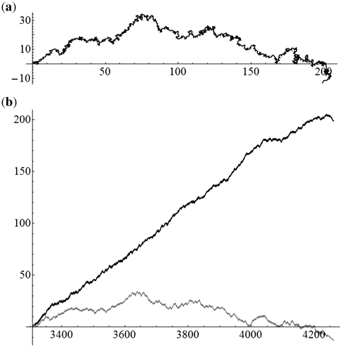
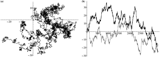
We first applied the SASR to simple DNA sequences, containing only a single coding or non-coding region, to investigate the behavior of the TP walk in these two special cases. Figure 3 shows the TP walk result of the first coding region (3307–4260) from the H. sapiens (Human) mitochondrial DNA sequence (No. J01415) and Figure 4 is the TP walk of the sequence before this region (1–3306, non-coding region without TP). In Figure 3a, the walk moves rightward from (0, 0) to around (200, 0) in the complex plane within only 954 steps, but in Figure 4a, the walk move around the zero point (Real part: −25–40; Imaginary part: −30–15) in the total 3306 steps. Meanwhile in Figure 3b, the real part keeps increasing with the growth of the t-value and the imaginary part keeps relatively constant. But in Figure 4b, both the real part and the imaginary part oscillate without a fixed pattern. Similar observations were found in experiments on other simple DNA sequences and it can be concluded that the TP walk of the single coding sequence has a trend moving rightward, while the walk of the non-coding sequence appears random. It is noticed that this principle is reasonable and is universally satisfied for such simple sequences, because it can be proved theoretically, as shown in Appendix 1.

Figure 3.

The TP walk of the first coding region (3307–4260) from the H. sapiens (Human) mitochondrial DNA sequence. (a) Walk trace in the complex plane. (b) Plot of the real part (black) and imaginary part (gray) of the points in the trace against the growing value of position t.

Figure 4.

The TP walk of the sequence before the first coding region (1–3306, non-coding region without TP property) of the H. sapiens (Human) mitochondrial DNA. (a) Walk trace in the complex plane. (b) Plot of the real part (black) and imaginary part (gray) of the points in the trace against the growing value of position t.

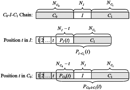
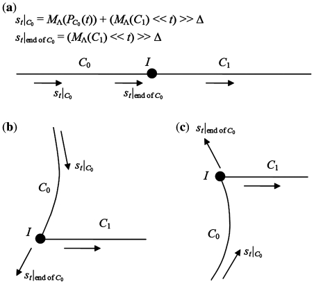
Consider a longer DNA sequence, which is a chain containing two coding regions with a non-coding region between them. This kind of chains is denoted as C₀-I-C₁ as shown in Figure 5. The two coding regions C₀ and C₁ are from a same organism, therefore share a same TP profile. Because we consider the coding regions’ general locations and the frame shift, rather than the exact boundaries, it is safe to assume that the lengths of C₀ and C₁ are multiples of 3, excluding the incomplete periods. Therefore the non-coding region I between them indicates a frame shift caused by insertions or deletions. The difference between the coding regions’ reading directions indicates a frame shift caused by an inversion. According to the definition of the TP sequence, which only takes the posterior subsequence into consideration, the walk in C₁ is not influenced by I or C₀, and it will be with the positive real direction as usual. However, walks in C₀ and I are influenced by their posterior parts, which are I-C₁ and C₁, respectively. From the detailed discussion in Appendix 2, we found that the walk in C₀ and I follows a fixed pattern. The walk in the I part is random around a relatively stable point, and the walk trace of the C₀ part is an arc. Therefore, it shows an obvious corner between the walk traces of C₀ and C₁. If C₀ and C₁ are in a same reading direction, there is a strong relationship between the frame shift value Δ and the corner’s shape, which is called here the ‘corner rule’ (Figure 6). Specifically, the change of the walk direction on the corner depends on Δ:

• Δ = 0: The direction keeps unchanged (go straight)

• Δ = 1: The direction rotates 2π/3 counterclockwise (turn left)

• Δ = 2: The direction rotates 2π/3 clockwise (turn right)

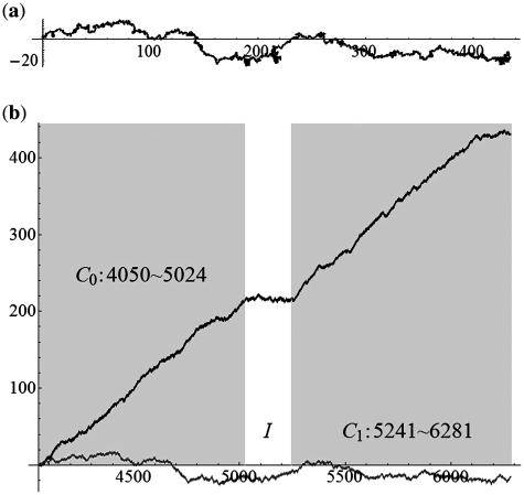
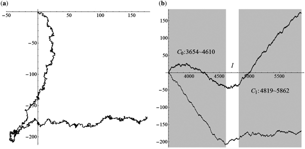
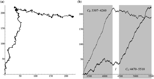
We applied the SASR to real C₀-I-C₁ chains with Δ = 0, 1, 2 (without inversion) to check whether the practical behavior conforms to the above discussion. Figure 7 shows the TP walk of a chain from the Gallus Gallus (Chicken) mitochondrial DNA sequence, which is with Δ = 0. Figure 8 shows the walk of a chain with Δ = 1, from the Halichoerus Grypus (Gray Seal) mitochondrial DNA and Figure 9 is for a chain with Δ = 2, from the H. sapiens (Human) mitochondrial DNA. Table 1 shows more details about these three chains. The (a) parts of Figures 7–9 indicate that the practical walk traces coincide with the corner rule. The (b) parts of Figures 7–9 show that the walks keep relatively constant in the non-coding regions compared with the high speed moving in the coding regions.

Figure 5.

C₀-I-C₁ Chain. N_* is the length of sub-sequence *.

Figure 6.

A sketch of the TP walk trace of the C₀-I-C₁ chain, when the two coding regions are in a same reading direction. (a) Δ = 0. (b) Δ = 1. (c) Δ = 2.

Figure 7.

The TP walk of 4050–6281 Gallus Gallus (Chicken) mitochondrial DNA sequence (Δ = 0). (a) Walk trace in the complex plane. (b) Plot of the real part (black) and imaginary part (gray) of the points in the trace against the growing value of position t and the dark areas stand for the coding regions.

Figure 8.

The TP walk of 3654–5862 Halichoerus grypus (Gray Seal) mitochondrial DNA sequence (Δ = 1). (a) Walk trace in the complex plane. (b) Plot of the real part (black) and imaginary part (gray) of the points in the trace against the growing value of position t and the dark areas stand for the coding regions.

Figure 9.

The TP walk of 3307–5510 H. sapiens (Human) mitochondrial DNA sequence (Δ = 2). (a) Walk trace in the complex plane. (b) Plot of the real part (black) and imaginary part (gray) of the points in the trace against the growing value of position t and the dark areas stand for the coding regions.

Table 1.

Three C₀-I-C₁ chains in real mitochondrial DNA sequences

Organism	Interval	C0	C1	Δ
Gallus Gallus (X52392)	4050–6281	4050–5024 (+)	5241–6281 (+)	0
Halichoerus Grypus (X72004)	3654–5862	3654–4610 (+)	4819–5862 (+)	1
Homo Sapiens (J01415)	3307–5510	3307–4260 (+)	4470–5510 (+)	2

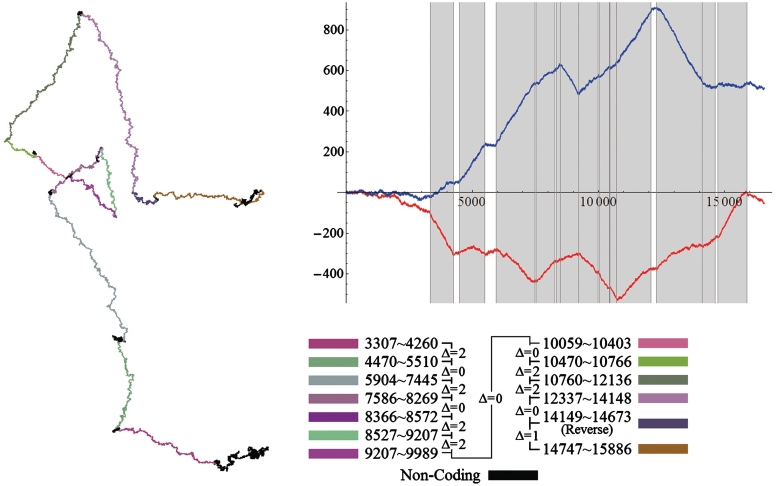
The practical TP walk for the complete DNA sequence was also investigated. Figure 10 shows the TP walk trace of the complete H. sapiens (Human) mitochondrial DNA sequence (No. J01415). The total 13 coding regions are marked in different colors and the Δ-value between each two of them is shown as well. It is clear in the figure that the coding regions stay on the arcs while the non-coding regions stay on the corners or around relatively stable points. The corners’ shapes follow the corner rule for all of the first 11 coding regions. The corner rule is not applicable for the two corners among 11th, 12th and 13th coding regions, because the 12th coding region is in the reverse reading direction. However, the 12th coding region also stays on an arc. Meanwhile, the top-right of Figure 10 shows that the curves of the real part and the imaginary part fluctuate up and down with the alternation of the coding regions and stay relatively constant in the non-coding regions. Actually, this behavior for the complete DNA sequence is raised by an accumulated effect of its short C₀-I-C₁ sub-chains from 3′ to 5′. It is easy to find that the TP walk of a complete sequence should follow the rules:

1. The walk traces of coding regions are arcs and the walk in the last coding region is with the positive real direction.

2. The walk in the non-coding regions is always random and moves around relatively stable points.

3. If two neighboring coding regions are in a same reading direction, the shape of the corner between them follows the corner rule.

Figure 10.

The TP walk trace of the complete H. sapiens (Human) mitochondrial DNA sequence in the complex plane with coding regions marked in different colors. The top-right is the plot of the real part (red) and imaginary part (blue) against the position value t and the dark areas stand for the coding regions.

The rule 3 is briefly proved in Appendix 3.

Performance and capability evaluations

Performance of the TP sequence’s generation algorithm

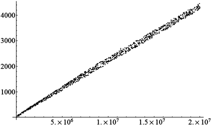
In order to test the practical computational complexity in generating a TP sequence from a DNA sequence, a simple program was written in the C++ language, and executed on a personal computer with Xeon(TM) CPU 2.8 GHz and 2.0 GB memory. We randomly generated 1000 artificial DNA sequences with random lengths (ranging from 20 000 to 2 00 000) and transformed them into TP sequences by using the algorithm mentioned in the ‘Materials and Methods’ section. The time cost of the 1000 transformations is plotted in Figure 11. It shows that the practical time cost rises from nearly 0 ms to 4200 ms with the sequence’s length N increasing from 20 000 to 2 00 000 linearly. It reveals that the practical computational complexity is O(N).

Figure 11.

Plot of the time cost against the sequence’s length N. The horizontal axis stands for the sequence’s length and the vertical axis stands for the time cost in millisecond.

The capability in discriminating coding and non-coding region

The TP walk visually discriminates the coding regions from the non-coding regions and also reveals the frame shift. However, it is significant to quantitatively investigate, to what extent, the TP walk’s patterns of the coding and non-coding regions are different, in order to check whether the coding regions can be further pointed out from the graph manually or computationally. Hence, we analyzed the difference between the walk’s patterns of two typical data sets. The data sets were extracted from the first 15 chromosome DNA sequences of the S. cerevisiae (no. NC_001133–NC_001147). One is called here the coding set or the positive set, containing all of the single-exon genes with ‘experimental evidence’. The other one is called the non-coding set or the negative set, containing all the inner sequences between genes. For a quantitative investigation, it needs to extract a measure from the SASR's visualization result, as a numerical representation of the walk’s pattern. For this reason, we present here a Rightward Rate (RR) measure. For a given DNA sequence, a RR measure is calculated from its TP walk W = {w_t | t = 0, 1, 2, … , N}:

(4)

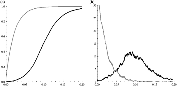
Here, Re(w) stands for the real part of the complex number w. This measure reveals the speed by which the walk moves rightward (with the positive real direction) in the complex plane. A single coding sequence has a TP walk moving rightward, causing the RR value being relatively high correspondingly. We applied the SASR on the sequences in the two data sets, and calculated their RR values. The Cumulative Distribution Function (CDF) and the Probability Density Functions (PDF) of the RR distributions in the two data sets are plotted in Figure 12. As expected, the non-coding sequences occupy the low RR area and the coding sequences tend to be with higher RR values. The sample means m and the sample standard deviations d are listed in Table 2. An independent 2-sample t-test was conducted on these two distributions, in which we got the t value at 107.069, and the P-value is ∼0. It indicates extreme high statistical significance of the difference between the two distributions.

Figure 12.

The RR distributions in the coding set (black) and the non-coding set (gray). (a) The CDF. (b) The PDF.

Table 2.

Statistics of measures for the two DNA sequences data sets

	Size	RR		OSCM		SRM
		m	d	m	d	m	d
Coding set (positive)	4144	0.10255	0.04444	0.00150	0.00099	0.04646	0.03289
Non-coding set (negative)	5594	0.02103	0.02401	0.00053	0.00221	0.01493	0.06558
Two-sample t-test
t-value		107.069		29.132		31.075
Degree of freedom		5924		8685		8207
P-value		0		6.18 × 10−178		2.00 × 10−201

The OSCM (27) and SRM (29) were also applied on the sequences in the two data sets. For the OSCM, the four coefficients have been set up, in Anastassiou’s work (27), as a = 0.1 + 0.12i, t = −0.3−0.2i, c = 0 and g = 0.45−0.19i, for the S. cerevisiae DNA. Meanwhile, we trained the SRM using the single-exon genes, which are with ‘experimental evidence’ and in the forward reading direction, from the 16th chromosomes of S. cerevisiae (no. NC_001148). Consider that, the OSCM and the SRM, set up from the genes in the forward direction, may miss the TP property in the reverse coding sequences, which are also contained in the positive set. To recognize such reverse TP property, in Anastassiou’s work (27) and Kotlar and Lavner’s work (29), the complementary measures were involved. According to Anastassiou (27), the four coefficients in the complementary measure are:  = t′e^−i2π/3,  = a′e^−i2π/3,  = g′e^−i2π/3 and  = c′e^−i2π/3. Here a′, t′, c′ and g′ are the complex conjugates of the original coefficients a, t, c, and g. In Kotlar and Lavner’s work (29), the complex coefficients of the four spectrums were also transformed in the same way to form the complementary measure. Therefore, the practical OSCM (or SRM) measure for discriminating the coding (in both reading directions) and non-coding sequences is the greater one between the original measure and its complementary measure. We calculated the OSCM and the SRM of each entire sequence in the two data sets and obtained the distributions of the measures’ values. The sample means and the sample standard deviations are also listed in Table 2. The t-tests obtained P-values at 6.18 × 10⁻¹⁷⁸ (OSCM) and 2.00×10⁻²⁰¹ (SRM) for the difference between the distributions of the positive and negative sets. Although they also show extreme high statistical significance of the difference, the P-values are higher and the t-values are much less than the corresponding values obtained by using the RR measure. It reveals that more obvious difference is obtained between the two data sets by using the SASR than using the OCSM and the SRM.

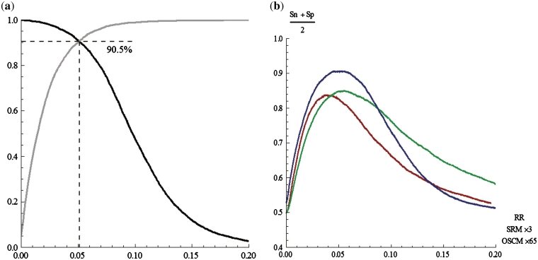
From another point of view, we investigated a classification of the sequences using a RR threshold, in which a sequence is classified to coding if its RR value is beyond the threshold x and non-coding otherwise. The sensitivity (Sn = number of correctly classified coding sequences/number of coding sequences) and the specificity (Sp = number of correctly classified non-coding sequences/number of non-coding sequences) (6,10,33) of this classification can be easily derived from the CDF of the two RR distributions mentioned above. That is Sn(x) = 1 – F_p(x) and Sp(x) = F_n(x), where F_p(x) and F_n(x) are the CDF of the RR distributions in the coding set and the non-coding set, respectively. The sensitivity and specificity are plotted in Figure 13a. It shows that, both the sensitivity and specificity can reach ∼90.5% at the RR threshold of ∼0.05, over all the samples. Meanwhile, the OSCM and the SRM were also used, instead of the RR measure, for the same classification. The sensitivity and specificity are also derived from the CDF of corresponding distributions. The averages of Sn and Sp by using these two measures are plotted in Figure 13b, as well as the corresponding value obtained by using the RR measure. It shows that, the peaks can reach only 83.5% and 85% by using the OSCM and the SRM, respectively, which show less accuracy, compared with using the RR measure.

Figure 13.

The accuracy in classifying sequences. (a) The sensitivity (black) and specificity (gray) in the classification by using the RR measure. (b) The averages of the sensitivity and specificity in the classification by using the OSCM (red), the SRM (green) and the RR measure (blue).

We catalogued the sequences by their length, and fixed the RR threshold at 0.05. It is found that the sensitivity in recognizing the long coding sequences is higher than in recognizing the short ones (Table 3), and the specificity shows a similar change over catalogs, except for a significant drop at the longest catalog, i.e. > 3300 bp. However, when the threshold is raised to 0.075, the coding regions in this catalog can be well discriminated with the Sn/Sp of 92.8/98.7%. It shows that the walk patterns of the very long (>3300 bp) coding and non-coding sequences still differ enough for the discrimination, and the low specificity when using the threshold of 0.05 may be caused by other periodicity patterns (not related to genetic coding). Beside, the precision (Pr = number of correctly classified coding sequences/number of classified coding sequences) (41) is also calculated. This value reflects the reliability of the classified coding sequences, which is impacted from the capability of the classification method as well as the coding/non-coding proportion of the data set. Table 3 shows that the precision is low in classifying sequences <600 bp, compared with the high value in the long length catalogs, although the very biased coding/non-coding proportion of the data set should also be noticed in the shortest and longest catalogs. In general, this test reveals that the TP walk is more capable in discriminating longer regions than the shorter ones, despite in the view of sensitivity, specificity or precision. This result is reasonable, because this approach is essentially to visualize the intensity of local TP and it requires a sufficient length to show such intensity, in statistics.

Table 3.

The sensitivity (Sn), specificity (Sp) and precision (Pr) in recognizing coding sequences with different lengths using the fixed RR threshold 0.05

Length	I	II (Sn) (%)	III	IV	V (Sp) (%)	VI	Pr (%)
1–300	89	66 (74.2)	23	2176	1813 (83.3)	363	15.4
301–600	463	364 (78.6)	99	1940	1602 (92.6)	338	51.8
601–900	612	524 (85.6)	88	710	694 (97.7)	16	97.0
901–1200	656	581 (88.6)	75	295	293 (99.3)	2	99.7
1201–1500	552	513 (92.9)	39	156	156 (100)	0	100
1501–1800	493	472 (95.7)	21	98	96 (98.0)	2	99.6
1801–2100	340	324 (95.3)	16	59	57 (96.6)	2	99.4
2101–2400	232	227 (97.8)	5	40	40 (100)	0	100
2401–2700	190	183 (96.3)	7	29	29 (100)	0	100
2701–3000	122	121 (99.2)	1	16	16 (100)	0	100
3001–3300	103	102 (99.0)	1	18	18 (100)	0	100
3301–∞	292	291 (99.5)	1	57	33 (57.9)	24	92.4
*3301–∞	292	271 (92.8)	21	57	56 (98.7)	1	99.6

I, Number of the coding sequences; II, number of the coding sequences classified as coding sequences; III, number of the coding sequences classified as non-coding sequences; IV, number of the non-coding sequences; V, number of the non-coding sequences classified as non-coding sequences; VI, number of the non-coding sequences classified as coding sequences. In the row with ‘asterisk’, threshold 0.075 is used.

The discussions presented above indicate that TP walk’s patterns of the coding and non-coding regions are different to a large extent for roughly distinguishing the coding regions manually or computationally.

DISCUSSION

There have been many studies visualizing various properties hidden in the DNA sequence, such as GC-AT walk (42), Z-curve representation (43) and Spider representation (44). Compared with these, the SASR's output, namely the TP walk, shows a better visual effect specifically for the TP property, which is strongly related to the protein coding. Therefore, the coding regions’ locations can be revealed directly from the TP walk trace (Figures 3 and 7–10). Meanwhile, according to Frenkel and Korotkov (15), most of the current Fourier transform-based methods do not allow revealing the frame shift between coding regions caused by insertions and deletions. In contrast, the SASR's output reveals such frame shift by the special corner’s shape (Figures 7–10).

As mentioned in the ‘Introduction’ section, most of the currently used methods, with outstanding performance in predicting coding regions, persistently depend on the preceding training process. They require a set of sufficient and suitable training data to obtain their high accuracies, otherwise, the methods may fail. Compared with them, the SASR does not require any extra information for training, since the vectors are rotated automatically with an auto-maintained TPM and the special selection process. Therefore, this approach is called ‘self adaptive’ and it facilitates the applications of the ‘TP profile matching’ on unknown organisms, which cannot provide sufficient known genes for the training. Moreover, as mentioned in the part of the capability evaluations, the OSCM and the SRM require another complementary predictor to detect the coding regions in the reverse reading direction (27,29). It is because the reverse coding regions contain the ‘reverse complementary’ TP profile. Using a single predictor may miss such TP property, if the trained profile is obtained from the forward reading genes. However, in the SASR, since the TPM is not obtained from any known genes, but automatically maintained, the reverse coding regions can be also visualized in a same TP walk with the forward regions (see the 12th region in Figure 10).

As mentioned in the ‘Introduction’ section, most of the ‘measure-based’ methods have limitations caused by the fixed analysis scale. Compared with the ‘measure-based’, the visualization is another way to analyze the TP property, providing opportunities to analyze sequences in various scales. The prediction of the coding regions can be obtained manually, taking advantages of human’s ‘auto-scale analysis ability’ or computationally, with some well developed time series theory or image processing methods.

CONCLUSION

This work proposes a new approach, named SASR, providing a visualized presentation of unannotated protein-coding regions in DNA sequences. This approach is based on the TP property, and using the Fourier transform. The graphic output (the TP walk) visually reveals the locations of the coding regions and the frame shifts between them: Arcs indicate the coding regions, stable points indicate the non-coding regions and the corners’ shapes reveal the frame shifts. Based on these visualized patterns, some computational methods can be further developed for various gene analysis purposes. In this work, we develop a preliminary TP score (the RR measure) based on the SASR, suitable in fast discrimination between relatively long coding and non-coding genomic sequences. Although our application on previously annotated genomic sequences shows clear potential of RR in the classification, further investigations are required in order to characterize the extent at which it can be applied in classical whole genome ab initio gene prediction analyses, concerning problems such as the choice of a proper threshold value.

In general, the SASR has some significant advantages including: (i) The SASR does not require any preceding training process, so it can work before any extra information is available, especially helpful when dealing with new sequences from unknown organisms; (ii) Without a fixed analysis scale, the visualization output provides opportunities to analyze sequences in various scales and take advantages of human’s ‘auto-scale analysis ability’; (iii) The SASR can be easily implemented with the computational complexity O(N). Hence, the SASR could be an efficient tool in investigation of the local TP property of genomic sequences, and further help in the ‘early stage’ gene prediction for new species having no annotated relatives. It is also helpful in the refinement of existing protein-coding regions annotation, because of its ability to detect frame shifts by mean of a visual inspection of the graphic output.

SUPPLEMENTARY DATA

Supplementary Data are available at NAR Online.

FUNDING

This work was supported by the Hong Kong Polytechnic University project (G-RPA7). Funding for open access charge: The Hong Kong Polytechnic University.

Conflict of interest statement. None declared.

APPENDIX 1

Consider the DNA sequence X with a TPM = {M_A(X), M_T(X), M_C(X), M_G(X)}^T. For each step t, the increment in equation 3 is:

Here, the ‘approximation ≈’ is because, in a single coding or non-coding DNA sequence, most of the posterior subsequences share the same entries’ proportions of TPM only with a shift caused by the position value t. Meanwhile, according to Frenkel and Korotkov (15), a certain base Λ appears at position j in the period with the probability:

Hence, for each step t, the increment of the TP walk is expected to be:

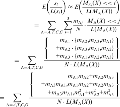(A.1)

Kotlar and Lavner’s work (29) shows that the entries in the TP vectors are biased in the single coding sequence, and uniformly random in the non-coding sequence. That is:

Then we have:

It shows that, in Equation A.1, for the single coding sequence, the third element of the expected increment dominates over the other two. According to equation 1, it causes the TP walk moving rightward in the complex plane. On the other hand, since the three vector’s elements are balanced for the non-coding sequence, the walk appears random around the zero point.

APPENDIX 2

First, we consider the walk in I, which is influenced by the posterior part C₁. Suppose that a base Λ appears at position t in the I part (Figure 5). Thus we have:

(A.2)

Here N_I means the length of the non-coding region I. According to the discussion in Appendix 1, the first term in the right hand side M_Λ(P_I(t)) is a complex random variable with the expected value of 0, since I is without TP property, and the three elements in this vector are balanced. Meanwhile M_Λ(C₁) is a non-zero constant vector, since C₁ is a coding region with TP property. However, because I is non-coding, the position where base Λ appears is uniformly random (29). It means that t is uniformly random, and so is N_I − t. Therefore, the second term M_Λ(C₁) >> (N_I − t) should be also random with the expected value of 0. So, in view of the total effect, the walk in this part should be random around a relatively stable point.

For the TP walk in C₀ part, we also suppose that a base Λ appears at position t in C₀ part (Figure 5). Thus we have:

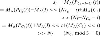(A.3)

Obviously, the first term in equation A.3 just indicates the original behavior of the TP walk in C₀ without the influence from I and C₁, and it is expected to be with the positive real direction as mentioned before. The second term is nearly 0, since there is no dominant element in M_Λ(I).

Now we focus on the third term in equation A.3. The difference between the coding regions’ reading directions reveals a frame shift caused by an inversion. There are two reading directions, i.e. the forward and reverse directions (43). There is no harm to assume that C₁ is in the forward direction, because if not, the derivation below is similar. It is noticed that, according to Kotlar and Lavner’s work (29), for a certain organism, base Λ has its preference position r_Λ (a real number in (0, 3] as an expected value) in the period. It causes M_Λ(C₁) to be with the expected phase angle of −2πr_Λ/3 in the complex plane. Then the behavior of the TP walk in C₀ is discussed in two cases as follows.

If C₀ is also in the forward direction, the preference position of Λ in C₀ is also r_Λ. Since t is just a position that Λ appears at, in view of the total effect, M_Λ(C₁) << t likely causes a same effect as M_Λ(C₁) << r_Λ does. It means a 2πr_Λ/3 counter clockwise rotation on M_Λ(C₁), which is with the expected phase angle of −2πr_Λ/3, and the production is with the expected phase angle of 0. In other words, M_Λ(C₁) << t is expected to be a positive real number. Then the direction of the third term only depends on the length of I, i.e. N_I. The frame shift between the two coding regions (without inversion) is Δ = N_I mod 3. It is easy to find that: if Δ = 0, the walk in C₀ will still be with the positive real direction, which is the same direction as in C₁. Otherwise, there will be a corner between the two coding regions, and the walk trace in C₀ will be an arc since the first term in equation A.3, M_Λ(P_C0(t)), becomes weaker and weaker with the growth of t, until the third term totally dominates in the s_t value at the end of C₀. At the end of C₀, the walk direction should only depend on the value of Δ. Accordingly, there is a strong relationship between Δ and the corner’s shape, which is called here the ‘corner rule’ (Figure 6). When the two neighboring coding regions (C₀ and C₁) are in a same reading direction, the change of the walk direction on the corner depends on Δ:

• Δ = 0: The direction keeps unchanged (go straight)

• Δ = 1: The direction rotates 2π/3 counterclockwise (turn left)

• Δ = 2: The direction rotates 2π/3 clockwise (turn right)

The corner rule satisfies only if the two coding regions are in a same reading direction. If C₀ is in the reverse reading direction (different from C₁), the triplets in C₀ are read from the complementary strand in the reverse direction (43). So the preference position of Λ in C₀ turns to be 4 − r_Λ′ (as the mirror image of r_Λ′ with the symmetry centre 2). Here Λ′ denotes the complementary base of Λ, i.e. A′ = T, T′ = A, G′ = C and C′ = G. Then in view of the total effect, M_Λ(C₁) << t is as the same as M_Λ(C₁) << (4 − r_Λ′) = M_Λ(C₁) << (1 − r_Λ′). It means a 2π(1 − r_Λ′)/3 counterclockwise rotation on M_Λ(C₁), and the production is with the expected phase angle of 2π(1 − r_Λ − r_Λ′)/3. In view of the total effect, the third term (M_Λ(C₁) << t) >> N_I has an expected direction. It reveals that the walk in C₀ part has its trend, and the walk trace also follows an arc. But the expected direction depends on some statistics of the organism besides a simple Δ value, including the proportions and the preference positions of the bases.

APPENDIX 3

Number the coding regions from the 5′-end to the 3′-end as C₀, C₁, … , C_K−1, C_K. Consider the corner between two neighbouring coding regions C_k−1 and C_k, which are both in the forward direction (the situation is similar if they are both in the reverse direction). Suppose that a base Λ appears at position t⁻ in C_k-1 and t⁺ in C_k, and these two positions are closed to the corner (t⁻and t⁺ are local index numbers for C_k−1 and C_k, namely t⁻ is nearly the length of C_k−1 and t⁺ is close to 0). Then we calculate the expected walk directions at these two positions.

Ignore the influence from the inner I parts since it is nearly 0 as discussed before, and also ignore the very short posterior subsequence at t⁻ in C_k−1 since position t⁻ is close to the corner (the end of C_k−1). Then we have:

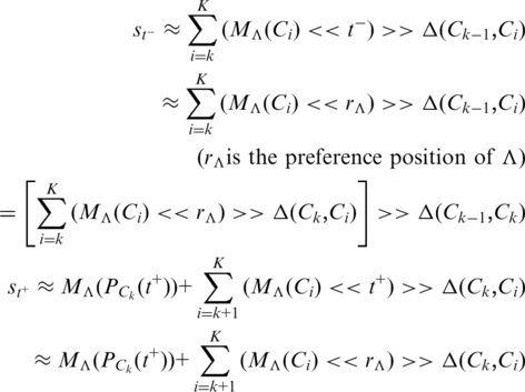Since t⁺ is close to the corner (the start of C_k), posterior subsequence at t⁺ in C_k is nearly the entire C_k with a shift. That is:

Accordingly,

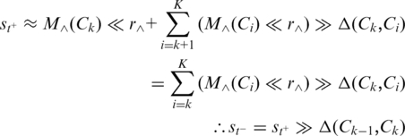It reveals that the walk direction rotates on the corner depending on Δ(C_k−1, C_k).

REFERENCES

- 1.Bennetzen JL, Hall BD. Codon selection in yeast. J. Biol. Chem. 1982;257:3026–3031. [PubMed] [Google Scholar]
- 2.Staden R, McLachlan AD. Codon preference and its use in identifying protein coding regions in long DNA sequences. Nucleic Acids Res. 1982;10:141–156. doi: 10.1093/nar/10.1.141. [DOI] [PMC free article] [PubMed] [Google Scholar]
- 3.Claverie JM, Bougueleret L. Heuristic informational analysis of sequences. Nucleic Acids Res. 1986;14:179–196. doi: 10.1093/nar/14.1.179. [DOI] [PMC free article] [PubMed] [Google Scholar]
- 4.Peng CK, Buldyrev SV, Goldberger AL, Havlin S, Sciortino F, Simons M, Stanley HE. Long-range correlations in nucleotide sequences. Nature. 1992;356:168–170. doi: 10.1038/356168a0. [DOI] [PubMed] [Google Scholar]
- 5.Li W. The complexity of DNA. Complexity. 1997;3:33–37. [Google Scholar]
- 6.Zhang CT, Wang J. Recognition of protein coding genes in the yeast genome at better than 95% accuracy based on Z curve. Nucleic Acids Res. 2000;28:2804–2814. doi: 10.1093/nar/28.14.2804. [DOI] [PMC free article] [PubMed] [Google Scholar]
- 7.Stanke M, Waack S. Gene prediction with a hidden Markov model and a new intron submodel. Bioinformatics. 2003;19:ii215–ii225. doi: 10.1093/bioinformatics/btg1080. [DOI] [PubMed] [Google Scholar]
- 8.Haimovich AD, Byrne B, Ramaswamy R, Welsh WJ. Wavelet analysis of DNA walks. J. Comput. Biol. 2006;13:1289–1298. doi: 10.1089/cmb.2006.13.1289. [DOI] [PubMed] [Google Scholar]
- 9.Orlov YL, Te Boekhorst R, Abnizova I. Statistical measures of the structure of genomic sequences: entropy, complexity and position information. J. Bioinform. Comput. Biol. 2006;4:523–526. doi: 10.1142/s0219720006001801. [DOI] [PubMed] [Google Scholar]
- 10.Te Boekhorst R, Abnizova I, Nehaniv C. Discriminating coding, non-coding and regulatory regions using rescaled range and detrended fluctuation analysis. BioSystems. 2008;91:183–194. doi: 10.1016/j.biosystems.2007.05.019. [DOI] [PubMed] [Google Scholar]
- 11.Do JH, Choi DK. Computational Approaches to Gene Prediction. J. Microbiol. 2006;44:137–144. [PubMed] [Google Scholar]
- 12.Borodovsky M, McIninch J. GeneMark: parallel gene recognition for both DNA strands. Comput. Chem. 1993;17:123–133. [Google Scholar]
- 13.Burge C, Karlin S. Prediction of complete gene structures in human genomic DNA. J. Mol. Biol. 1997;268:78–94. doi: 10.1006/jmbi.1997.0951. [DOI] [PubMed] [Google Scholar]
- 14.Salzberg S, Delcher A, Kasif S, White O. Microbial gene identification using interpolated Markov models. Nucleic Acids Res. 1998;26:544–548. doi: 10.1093/nar/26.2.544. [DOI] [PMC free article] [PubMed] [Google Scholar]
- 15.Frenkel FE, Korotkov EV. Classification analysis of triplet periodicity in protein-coding regions of genes. Gene. 2008;421:52–60. doi: 10.1016/j.gene.2008.06.012. [DOI] [PubMed] [Google Scholar]
- 16.Frenkel FE, Korotkov EV. Using triplet periodicity of nucleotide sequences for finding potential reading frame shifts in genes. DNA Res. 2009;16:105–114. doi: 10.1093/dnares/dsp002. [DOI] [PMC free article] [PubMed] [Google Scholar]
- 17.Fickett JW. The gene identification problem: An overview for developers. Comput. Chem. 1996;20:103–118. doi: 10.1016/s0097-8485(96)80012-x. [DOI] [PubMed] [Google Scholar]
- 18.Fickett JW. Recognition of protein coding regions in DNA sequences. Nucleic Acids Res. 1982;10:5303–5318. doi: 10.1093/nar/10.17.5303. [DOI] [PMC free article] [PubMed] [Google Scholar]
- 19.Henderson J, Salzberg S, Fasman KH. Finding Genes in DNA with a Hidden Markov Model. J. Comput. Biol. 1997;4:127–141. doi: 10.1089/cmb.1997.4.127. [DOI] [PubMed] [Google Scholar]
- 20.Azad RK, Borodovsky M. Probabilistic methods of identifying genes in prokaryotic genomes: Connections to the HMM theory. Brief. Bioinform. 2004;5:118–130. doi: 10.1093/bib/5.2.118. [DOI] [PubMed] [Google Scholar]
- 21.Cao YH, Tung WW, Gao JB, Qi Y. Recurrence time statistics: Versatile tools for genomic DNA sequence analysis. J. Bioinform. Comput. Biol. 2005;3:677–696. doi: 10.1142/s0219720005001235. [DOI] [PubMed] [Google Scholar]
- 22.Gao JB, Qi Y, Cao YH, Tung WW. Protein coding sequence identification by simultaneously characterizing the periodic and random features of DNA sequences. J. Biomed. Biotechnol. 2005;2005:139–146. doi: 10.1155/JBB.2005.139. [DOI] [PMC free article] [PubMed] [Google Scholar]
- 23.Tiwari S, Ramachandran S, Bhattacharya A, Bhattacharya S, Ramaswamy R. Prediction of probable genes by Fourier analysis of genomic sequences. Comput. Appl. Biosci. 1997;13:263–270. doi: 10.1093/bioinformatics/13.3.263. [DOI] [PubMed] [Google Scholar]
- 24.Yan M, Lin ZS, Zhang CT. A new Fourier transform approach for protein coding measure based on the format of the Z curve. Bioinformatics. 1998;14:685–690. doi: 10.1093/bioinformatics/14.8.685. [DOI] [PubMed] [Google Scholar]
- 25.Dodin G, Levoir P, Cordier C. Triplet correlation in DNA sequences and stability of heteroduplexes. J. Theor. Biol. 1996;183:341–343. doi: 10.1006/jtbi.1996.0225. [DOI] [PubMed] [Google Scholar]
- 26.Dodin G, Vandergheynst P, Levoir P, Cordier C, Marcourt L. Fourier and wavelet transform analysis, a tool for visualizing regular patterns in DNA sequences. J. Theor. Biol. 2000;206:323–326. doi: 10.1006/jtbi.2000.2127. [DOI] [PubMed] [Google Scholar]
- 27.Anastassiou D. Frequency-domain analysis of biomolecular sequences. Bioinformatics. 2000;16:1073–1081. doi: 10.1093/bioinformatics/16.12.1073. [DOI] [PubMed] [Google Scholar]
- 28.Anastassiou D. Genomic Signal Processing. Bioinf. Signal Process. Mag. 2001;18:8–20. [Google Scholar]
- 29.Kotlar D, Lavner Y. Gene prediction by spectral rotation measure: a new method for identifying protein-coding regions. Genome Res. 2003;13:1930–1937. doi: 10.1101/gr.1261703. [DOI] [PMC free article] [PubMed] [Google Scholar]
- 30.Masoom H, Datta S, Asif A, Cunningham L, Wu G. In Proceedings of the IEEE Symposium on Computational Intelligence and Bioinformatics and Computational Biology. Toronto, Canada: 2006. A fast algorithm for detecting frame shifts in DNA sequences; pp. 1–8. [Google Scholar]
- 31.Tuqan J, Rushdi A. Proceedings of the 40th Asilomar Conference on Signals, Systems and Computers. Pacific Grove, California: 2006. The filtered spectral rotation measure; pp. 1875–1879. [Google Scholar]
- 32.Tuqan J, Rushdi A. A DSP Approach for Finding the Codon Bias in DNA Sequences. IEEE J. Sel. Top. Sign. Proces. 2008;2:343–356. [Google Scholar]
- 33.Yin CC, Yau Stephen ST. Prediction of protein coding regions by 3-base periodicity analysis of a DNA sequence. J. Theor. Biol. 2007;247:687–694. doi: 10.1016/j.jtbi.2007.03.038. [DOI] [PubMed] [Google Scholar]
- 34.Jiang XY, Lavenier D, Yau Stephen ST. Coding region prediction based on a universal DNA sequence representation method. J. Comput. Biol. 2008;15:1237–1256. doi: 10.1089/cmb.2008.0041. [DOI] [PubMed] [Google Scholar]
- 35.Chang CQ, Fung Peter CW, Hung YS. In Proceedings of the Fifth International Conference on Information Technology and Application in Biomedicine, in conjunction with the Second International Symposium and Summer School on Biomedical and Health Engineering. Shenzhen, China: 2008. Improved gene prediction by resampling-based spectral analysis of DNA sequence; pp. 221–224. [Google Scholar]
- 36.Akhtar M, Ambikairajah E, Epps J. Processing of IEEE International Conference on Acoustics, Speech and Signal Processing. Las Vegas, Nevada, USA: 2008. Optimizing period-3 methods for eukaryotic gene prediction; pp. 621–624. [Google Scholar]
- 37.Akhtar M, Epps J, Ambikairajah E. Signal processing in sequence analysis: advances in eukaryotic gene prediction. IEEE J. Sel. Top. Sign. Proces. 2008;2:310–321. [Google Scholar]
- 38.Ré M, Pavesi G. Detecting conserved coding genomic regions through signal processing of nucleotide substitution patterns. Artif. Intell. Med. 2009;45:117–123. doi: 10.1016/j.artmed.2008.07.015. [DOI] [PubMed] [Google Scholar]
- 39.Voss RF. Evolution of long-range fractal correlations and 1/f noise in DNA base sequences. Phys. Rev. Lett. 1992;68:3805–3808. doi: 10.1103/PhysRevLett.68.3805. [DOI] [PubMed] [Google Scholar]
- 40.Fickett JW, Tung CS. Assessment of protein coding measures. Nucleic Acids Res. 1992;20:6441–6450. doi: 10.1093/nar/20.24.6441. [DOI] [PMC free article] [PubMed] [Google Scholar]
- 41.Olson DL, Delen D. Advanced Data Mining Techniques. Springer: Berlin Heidelberg; 2008. [Google Scholar]
- 42.Berthelsen CL, Glazier JA, Skolnick MH. Global fractal dimension of human DNA sequences treated as pseudorandom walks. Phys. Rev. A. 1992;45:8902–8913. doi: 10.1103/physreva.45.8902. [DOI] [PubMed] [Google Scholar]
- 43.Zhang R, Zhang CT. Z-curves, an intutive tool for visualizing and analyzing the DNA sequences. J. Biomol. Struct. Dyn. 1994;11:767–782. doi: 10.1080/07391102.1994.10508031. [DOI] [PubMed] [Google Scholar]
- 44.Cebrat S, Dudek MR. The effect of DNA phase structure on DNA walks. Eur. Phys. J. B. 1998;3:271–276. [Google Scholar]
Associated Data
This section collects any data citations, data availability statements, or supplementary materials included in this article.