PDE-constrained multispectral imaging of tissue chromophores with the equation of radiative transfer

Abstract

We introduce a transport-theory-based PDE-constrained multispectral model for direct imaging of the spatial distributions of chromophores concentrations in biological tissue. The method solves the forward problem (boundary radiance at each wavelength) and the inverse problem (spatial distribution of chromophores concentrations), in an all-at-once manner in the framework of a reduced Hessian sequential quadratic programming method. To illustrate the code’s performance, we present numerical and experimental studies involving tumor bearing mice. It is shown that the PDE-constrained multispectral method accelerates the reconstruction process by up to 15 times compared to unconstrained reconstruction algorithms and provides more accurate results as compared to the so-called two-step approach to multi-wavelength imaging.

1. Introduction

Over the past decade near-infrared optical tomography (NIROT) has emerged as a viable imaging modality to monitor physiologically important parameters such as concentrations of oxyhemoglobin [HbO₂] and deoxyhemoglobin [Hb] in tissues [1–8]. This technique extracts tissue chromophore concentrations by exploiting the absorption data at multiple wavelengths, based on the fact that absorbers in tissue such as hemoglobin, water and lipid are linearly correlated with the tissue absorption. Initially researchers employed the so-called two-step method to obtain the concentrations of these absorbers and other chromophores. In this approach, the absorption coefficients are retrieved sequentially for each wavelength and then combined to obtain the concentrations through a direct matrix inversion or a least-squared method. However, it is well known [4,6,7] that this two-step approach sometimes produces unreasonable results (e.g. negative chromophore concentrations), and can show strong cross-talk between chromophores. To overcome this problem, researchers introduced a multispectral method in which chromophore concentrations are directly reconstructed by utilizing spectral constraints between chromophores into the reconstruction process. It has been shown that these direct methods provide improved accuracy and mitigate cross-talk. Li et al. [6] proposed a multispectral method based on the perturbation theory and demonstrated that it improved the concentration images of various chromophores. Corlu et al. [4,7] explored wavelength optimization for the continuous-wave multispectral optical tomography and validated their results through numerical simulations and with experimental data.

Both Li et al. and Corlu et al., however, based their work on the diffusion approximation (DA) to the more generally applicable equation of radiative transfer (ERT). It is well known that the diffusion approximation becomes less accurate when applied to imaging of small-tissue volumes and is further compromised if highly absorbing objects or fluid-filled regions, which contain, for example, cerebrospinal or synovial fluids, are considered [9]. The use of the full ERT alleviates these problems and provides accurate prediction of intensity measurements for imaging of small-tissue geometries. However, employing the ERT with the conventional two-step approach leads to prohibitively long computation times compared to the DA version, since the two-step model requires a large number of repeated forward simulations (based on ERT) that should be done for each wavelength during optimization. Thus it remains a challenging task to develop computationally efficient, accurate transport-theory-based multispectral chromophore reconstruction codes. This motivates our implementation of a fast ERT-based multispectral model for direct accurate imaging of chromophores concentrations in small-tissue volumes.

In this work we present a novel approach called a PDE-constrained multispectral imaging method that enables us to achieve two goals: first this approach accelerates the ERT-based image reconstruction process, and second it improves the chromophore reconstruction accuracy. To evaluate the new method, we provide numerical simulations and experimental results involving tumor bearing mice. Throughout these studies our new method is compared to the performance of the conventional unconstrained two-step method.

2. Equation of radiative transfer as a light propagation model

The frequency domain forward model for light propagation in tissue can be accurately modeled by the radiative transfer equation [10,11] as

$$[\Omega \cdot \nabla +{\mu }_a(\lambda )+{\mu }_s(\lambda )+i\frac{\omega }{c}]u_{\lambda }(\overrightarrow{r},\Omega ,\omega )=\frac{{\mu }_s^{\lambda }}{4\pi }{\displaystyle \underset{4\pi }{\int }{u}_{\lambda }(\overrightarrow{r},{\Omega }^{+},\omega )}\Phi ({\Omega }^{+},\Omega )d{\Omega }^{+}+Q_{\lambda }(\overrightarrow{r},\Omega ,\omega )$$ (1)

where u_λ is the spectral radiation intensity in unit [W/cm²/sr./nm], Q_λ is the interior spectral radiation source in unit [W/cm³/sr./nm], and μ_a(λ) and μ_s(λ) are the wavelength-dependent absorption and scattering coefficient in unit [1/cm], and Φ is the phase function describing scattering from direction Ω⁺ into direction Ω. We use here the Henyey-Greenstein phase function that is commonly used in tissue optics. The above equation can be solved with appropriate boundary conditions. In this work, we implemented a partially-reflective boundary condition [12] that allows us to consider the refractive index mismatch between the tissue and air.

We use an unstructured node-centered finite-volume approach [11] for the angular domain and a discrete ordinates formulation for the spatial domain, in order to obtain the discretized form of Au = b where the sparse matrix A contains all coefficients resulting from discretization and the vector b represents the discretized boundary conditions, respectively. The algebraic equation Au = b, is solved with a complex version of the GMRES (m) linear solver [13] where m denotes the iteration number after which GMRES is restarted. Thus, the spectral intensity and phase shift are obtained by solving the forward problem [Eq. (1)] with a distribution of known optical properties at wavelength λ.

The tissue chromophore reconstruction is based on the linear correlation between the absorption coefficient and the chromophore concentration. The known mapping function of the i-th chromophore concentration C_i to the absorption coefficient μ_a(λ) is given with the i-th absorption extinction coefficient ε_i(λ) as

$${\mu }_a(\lambda )={\displaystyle \sum _{i=1}^{N_c}{\epsilon }_i(\lambda )C_i}$$ (2)

where N_c is the number of total chromophores that contribute to the absorption at wavelength λ. In the matrix form, Eq. (2) is given as [M] = [E][C] where the coefficient matrix [E] denotes the molar extinction coefficients of chromophores whose values are available in the literature [14], and the concentration vector [C] denotes the concentration of chromphores.

3. Two-step and multi-spectral PDE-constrained models

Reconstruction of tissue chromophore concentrations can be performed in two different ways: a two-step method or a one-step multispectral method. Both methods will be described in some detail next.

3.1 Two step Method

The traditional two-step method deals with reconstructing the absorption data μ_a(λ) for each wavelength λ which corresponds to minimizing the objective function defined at wavelength λ given as

$$\varphi [{\mu }_a({\lambda }_n),{\mu }_s({\lambda }_n)]=\frac{1}{2}{\displaystyle \sum _{d=1}^{ND}{\left|Q{u}_d^{\lambda }-z_d^{\lambda }\right|}^2}.$$ (3)

where Q is the measurement operator that projects the angular intensity distribution $u_d^{\lambda }$ onto the measurable quantity (i.e., radiation flux at the surface), $z_d^{\lambda }$ is the spectral measurement made at surfaces and ND is the total number of measurements. Then these images are converted into the chromophore concentration images. For example, consider four main absorbers (HbO₂, Hb, Water and Lipid) with four wavelengths measurements. In this case, we can decompose four absorption coefficient maps into into the chromophore images by using Eq. (2) as

$$\left[\begin{array}{l}{\text{HbO}}_{\text{2}}\\ \text{Hb}\\ \text{Water}\\ \text{Lipid}\end{array}\right]={\left[\begin{array}{cccc}{\epsilon }_{{\text{HbO}}_{\text{2}}}^{{\lambda }_1}& {\epsilon }_{\text{Hb}}^{{\lambda }_1}& {\epsilon }_{\text{Water}}^{{\lambda }_1}& {\epsilon }_{\text{Lipid}}^{{\lambda }_1}\\ {\epsilon }_{{\text{HbO}}_{\text{2}}}^{{\lambda }_2}& {\epsilon }_{\text{Hb}}^{{\lambda }_2}& {\epsilon }_{\text{Water}}^{{\lambda }_2}& {\epsilon }_{\text{Lipid}}^{{\lambda }_2}\\ {\epsilon }_{{\text{HbO}}_{\text{2}}}^{{\lambda }_3}& {\epsilon }_{\text{Hb}}^{{\lambda }_3}& {\epsilon }_{\text{Water}}^{{\lambda }_3}& {\epsilon }_{\text{Lipid}}^{{\lambda }_3}\\ {\epsilon }_{{\text{HbO}}_{\text{2}}}^{{\lambda }_4}& {\epsilon }_{\text{Hb}}^{{\lambda }_4}& {\epsilon }_{\text{Water}}^{{\lambda }_4}& {\epsilon }_{\text{Lipid}}^{{\lambda }_4}\end{array}\right]}^{-1}\left[\begin{array}{c}{\mu }_a({\lambda }_1)\\ \begin{array}{l}{\mu }_a({\lambda }_2)\\ {\mu }_a({\lambda }_3)\end{array}\\ {\mu }_a({\lambda }_4)\end{array}\right]$$ (4)

If more than four wavelengths are used to obtain four chromophores, i.e., N_c < N_λ, the chromophore concentrations may be the least-squared solutions to Eq. (2).

The one-step multispectral method retrieves the spatial distributions of chromphore concentrations directly by employing the multispectral measurements simultaneously into reconstruction. This can be achieved by minimizing the sum of the objective functions defined at each wavelength λ as:

$$f(C_i)={\displaystyle \sum _{n=1}^{N_{\lambda }}\varphi [{\mu }_a({\lambda }_n),{\mu }_s({\lambda }_n)]}=\frac{1}{2}{\displaystyle \sum _{n=1}^{N_{\lambda }}{\displaystyle \sum _{d=1}^{ND}{\left|Q{u}_d^{{\lambda }_n}-z_d^{{\lambda }_n}\right|}^2}}$$ (5)

where N_λ is the number of measurement wavelengths and C_i is the i-th chromophore concentration that can be either [HbO₂] or [Hb] or [Water] or [Lipid] concentrations. Note that the reconstruction variables in Eq. (5) are the chromophore concentrations themselves, not the absorption coefficients. Equation (5) also shows that the chromophore concentrations are updated by checking variations in all spectral data through the minimization process. Since the multispectral method can make use of as many wavelength data as available for the same number of unknowns, it improves the nature of the problem, thus making a highly ill-posed problem less ill-posed. This cannot be achieved by the two-step method, which just increases the number of unknowns as the number of measurement wavelengths is increased.

3.2 PDE-constrained multispectral method

We introduce here the PDE-constrained multispectral model. In order to understand the difference between the PDE-constrained multispectral and standard PDE-constrained models, we begin with a brief review of the standard PDE-constrained optimization.

Consider the standard optical tomographic problem defined at each wavelength as:

$$\text{min }f({\mu }_{\lambda };u_{\lambda })=\frac{1}{2}{\left|Q{u}_{\lambda }-z_{\lambda }^{obs}\right|}^2+\beta R\text{ subject to }c({\mu }_{\lambda };u_{\lambda })=A{u}_{\lambda }-b=0$$ (6)

where u and z^obs denote the vectors of spectral intensity predictions and measurements, respectively, R denotes appropriate regularization with a regularization parameter β, and μ_λ denotes a vector of unknown wavelength-dependent absorption coefficients. The equation Au = b is a discretized version of the forward transport equation. The problem given by Eq. (6) is often referred to as “PDE-constrained” since the optimal solution at minimum of f has to satisfy the partial differential equations (i.e., ERT) represented by Au = b.

The most common approach for solving Eq. (6) is to treat the forward variable u as a dependent variable of the inverse variable μ_λ, which makes it possible to replace the prediction vector u in f of Eq. (6) by its forward solution vector A⁻¹b. As a result, the problem Eq. (6) is reformulated as

$$\text{minimize }{f}^{\ast }({\mu }_{\lambda })=\frac{1}{2}{\left|Q{A}^{-1}b-z_{\lambda }^{obs}\right|}^2+\beta R$$ (7)

which is often referred to as “unconstrained” because equality Au = b no longer appears in Eq. (7), i.e., f* is now a function of μ_λ only. Thus the accurate forward solution A⁻¹b has to be obtained for each wavelength λ for evaluation of the objective function Eq. (7), which makes the unconstrained code computationally very expensive both with respect to time and memory. Nonetheless, this approach has been widely used in optical tomography because of the ease of implementation. The existing DA-based multispectral or two-step schemes [2–7] belong to this category.

Another approach to solve Eq. (6), is to treat the forward variable u and the inverse variable μ_λ independently. This enables solving the equality-constrained problem [Eq. (6)] directly by updating the forward and inverse variables simultaneously at each of optimization iterations. Typically the PDE-constrained inverse problem [Eq. (6)] can be reformulated into the framework of the following extended objective function called “Lagrangian” as:

$$L({\mu }_{\lambda },u_{\lambda };{\eta }_{\lambda })\triangleq \frac{1}{2}{\left|Q{u}_{\lambda }-z_{\lambda }^{obs}\right|}^2+{\eta }_{\lambda }^T(A{u}_{\lambda }-b)$$ (8)

Here η is called the vector of Lagrange multipliers. The simultaneous solutions of forward and inverse problems can be achieved at points satisfying the so-called first order Karush-Khun-Tucker (KKT) conditions [11,15] where the gradient of L in Eq. (8) vanishes with respect to η, u and μ_λ, respectively. One major advantage of this PDE-constrained approach is that the solution of the forward problem does not have to be accurate until optimization reaches convergence. So the inexact solution obtained with a loose criterion can be used into optimization, which leads to a significant saving in the total reconstruction time. Recently, our group has for the first time used this PDE-constrained optimization into imaging of absorption and scattering maps in tissue: the augmented Lagrangian (AL) method [15] and the reduced Hessian sequential quadratic programming (rSQP) method [11].

However, the PDE-constrained approach of this kind [Eq. (8)] cannot be used directly with the one-step multispectral model. The reason is that the standard PDE-constrained optimization method [Eq. (8)] works only for a single wavelength-dependent constrained problem [Eq. (6)]. Thus it cannot treat all wavelengths data simultaneously within a PDE-constrained optimization framework. Therefore the standard PDE-constrained optimization approach has to be reformulated into a one-step multispectral model so that all multispectral data can be utilized simultaneously into reconstruction, which is the focus of this study.

In the following we provide a description of the formulation of PDE-constrained multispectral optimization. The basic idea behind this new method is to combine the multispectral model [Eq. (5)] and the PDE-constrained approach [Eq. (8)]. In other words, to be able to use data from all wavelengths we minimize the sum of the objective function defined at each wavelength λ [Eq. (5)] within the framework of PDE-constrained optimization [Eq. (8)]. This is achieved with the following formulations for PDE-constrained multispectral optimization:

$$\text{min }f(x;u_{\lambda })=\frac{1}{2}{\displaystyle \sum _{\lambda }{\left|Q{u}_{\lambda }-z^{obs}\right|}^2}+\beta R(x)\text{ subject to }c(x;u_{\lambda })=A{u}_{\lambda }-b=0$$ (9)

$$L(x,u_{\lambda };{\eta }_{\lambda })\triangleq \frac{1}{2}{\displaystyle \sum _{\lambda }{\left|Q{u}_{\lambda }-z_{\lambda }^{obs}\right|}^2}+{\displaystyle \sum _{\lambda }{\eta }_{\lambda }^T(A{u}_{\lambda }-b)}$$ (10)

Here the inverse variable becomes a vector x of all unknown chromophore concentrations, i.e., x = (C_j). We employ here the rSQP method to solve the PDE-constrained multispectral problem [Eq. (9)] by minimizing the multispectral Lagrangian function L [Eq. (10)] with respect to η, u and x. A multispectral version of the rSQP algorithm is described in the following section.

3.3 Reduced Sequential Quadratic Programming (rSQP)

In the PDE-constrained multispectral model, the reduced Hessian SQP scheme solves the optimization problem [Eq. (9)] by minimizing the quadratic approximation of the Lagrangian function given by Eq. (10) subject to the linearization of the forward equation as follows:

$$\text{min }\Delta x^{kT}{g}_r^k+\frac{1}{2}\Delta x^{kT}{H}_r^k\Delta x^k\text{ subject to }{C}^k\Delta p^k+{(A{u}_{\lambda }-b)}^k=0$$ (11)

where Δp = (Δx, Δu_λ)^T at (x^k, u_λ^k), $g_r^k$is the reduced gradient and $H_r^k$ is the reduced Hessian of the Lagrangian function. Here $C^k$denotes the Jacobian matrix of the constraint with respect to p = (x, u_λ), given by $C^k={(A{u}_{\lambda }-b)}_p^{kT}$. After differentiation of Eq. (11) with respect to Δx, we finally can obtain the following forms for the updates of forward and inverse variables as:

$$\begin{array}{l}\Delta x^k=-{\left(H_r^k\right)}^{-1}{g}_r^k\\ \Delta u_{\lambda }^k=A^{-1}\left[{(A{u}_{\lambda })}^k-b-{\left(A{u}_{\lambda }\right)}_x^{kT}\Delta x^k\right]\end{array}$$ (12)

where the matrix-vector product ${(H_r^k)}^{-1}{g}_r^k$ is directly approximated by using the limited-memory BFGS updating formula [16]. Here the reduced gradient $g_r^k$ is given for the j-th chromophore concentration as:

$$g_{r,j}^k={\displaystyle \sum _{\lambda }{\epsilon }_j^{\lambda }\left(u_{\lambda }^{kT}{A}_{x_j}^T{\eta }_{\lambda }^k\right)+}{\nabla }_{x_j}{f}^k$$ (13)

The Lagrangian multiplier ${\eta }_{\lambda }^k$ at each wavelength λ can be obtained by solving the corresponding adjoint equation, given as:

$$A^{kT}{\eta }_{\lambda }^k=-Q^T{(Q{u}_{\lambda }^k-z_{\lambda }^{obs})}^{*}$$ (14)

where the operator (.)* denotes the complex conjugate of the complex vector. The global convergence of the PDE-constrained multispectral algorithm is ensured by a line search on the following $l_1$ merit function that somehow balances the aims of reducing the objective function and satisfying the constraints, given as:

$${\phi }_{{\eta }_k}(u_{\lambda },x)=f(u_{\lambda },x)+{\displaystyle \sum _{\lambda }{\eta }_{\lambda }{\Vert A{u}_{\lambda }-b\Vert }_1}$$ (15)

which is chosen here for its simplicity and low computational cost. The merit function [Eq. (15)] is successively monitored to ensure the global progress towards the optimal forward and inverse solutions, while a line search is performed to find a step length ${\alpha }^k$ that can provide a sufficient decrease in the merit function. As a consequence, the new iterate is given as:

$$\begin{array}{l}{x}^{k+1}=x^k+{\alpha }^k\Delta x\\ u_{\lambda }^{k+1}=u_{\lambda }^k+{\alpha }^k\Delta u_{\lambda }^k.\end{array}$$ (16)

The algorithm as described in Eqs. (11)–(16) is used for our numerical and experimental studies that will be presented next.

4. Results

In this section, we apply the newly developed PDE-constrained multispectral method to directly recover the chromphore concentrations inside the medium. The performance of the algorithm is evaluated in terms of CPU times and accuracy. Without loss of generality, the scattering coefficient was assumed to be constant over the medium, given by μ_s^′(λ) = Aλ^-b (A = 45000, b = 1.3). In both the numerical and the experimental studies, we focus on the reconstruction of the oxy-hemoglobin (HbO₂) and deoxy-hemoglobin (Hb) concentrations since these are two major absorbers in tissue closely related to disease progression and physiological process. Water concentration was assumed constant over the medium.

4.1 Numerical study

First, we consider two-dimensional circular enclosure, as shown in Fig. 1 , filled with an inhomogeneous medium. Two objects with a diameter of 0.2cm are embedded in the background: one differs only in [HbO₂] and the one only in [Hb]. The corresponding chromophore concentrations are given in Table 1 for the background medium and the objects. The background medium has [HbO₂] of 40[μM] and [Hb] of 20[μM]. The object 1 has [HbO₂] of 80 while the object 2 has [Hb] of 40[μM]. These values are chosen here to mimic absorption coefficients of 0.1~0.2 (cm⁻¹), which correspond to the typical transport regime.

Fig. 1.

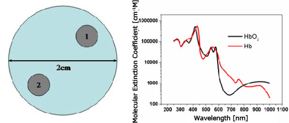
Circular enclosure (left) and absorption spectra of HbO₂ (right): the test medium has two objects of perturbation: one in [HbO₂] and one in [Hb].

Table 1. Chromophore concentrations and optical properties of the background medium and the objects.

Object	HbO2 [μM]	Hb [μM]	Water [%]
Background	40	20	18
1	80	20	18
2	40	40	18

Eight sources are located around the enclosure surface at regular intervals. The sources are isotropic-emitting into the medium and intensity-modulated with a frequency of 600 MHz. The 64 detectors are equally spaced around the boundary surface. This yields a total of 512 source-detector pairs for reconstruction. For noise-free simulated data z_d in Eq. (5), we used a mesh of 11538 triangle elements with a S₁₀ quadrature. The prediction Qu_d in Eq. (5) is obtained on a coarser mesh of 2854 triangular elements with a S₆ quadrature. Measurements containing noise are simulated by adding an error term to z_d in the form $z_d^{obs}=z_d+\varpi \sigma$, where σ is the standard deviation of measurement errors and ϖ is the random variable with normal distribution. Here we chose a noise level of 15dB which represents the typical noise level encountered in optical tomography [17].

Since we look at the reconstruction of [HbO₂] and [Hb], we only need two wavelengths to distinguish between these two chromophores. However, different sets of two wavelengths may affect the reconstruction accuracy. To illustrate the influence of the wavelengths set chosen, we consider two different sets of measurement wavelengths which are selected here from commonly available diode lasers: one set with (650nm, 830nm), the other set with (760nm, 830nm). Another reason for this set comes from the fact that, as shown in Fig. 1, the molar extinction coefficients of HbO₂ and Hb are different from each other for chosen wavelengths, which is thus believed to be favorable to reconstructing HbO₂ and Hb concentrations.

We use two metrics for the reconstruction quality: a correlation coefficient ρ_c and a deviations factor ρ_d, as defined in [17]. Accordingly, the larger correlation coefficient, close to 1, and smaller deviation factor, close to zero, represents the higher accuracy. Also the correlation coefficient may be used to indicate the degree of cross-talk that can be measured as the HbO₂ (Hb) concentration divided by the Hb (HbO₂) concentration in Hb (HbO₂) position of the known object. Besides the effects of different wavelength sets, we also investigate the CPU times in both PDE-constrained and conventional multispectral methods, which is another important metric for evaluation of the performance of the proposed algorithm. All reconstructions are performed using two methods: the PDE-constrained one-step multispectral method and the unconstrained two-step method. Note that the unconstrained two-step method is based on the quasi-Newton (BFGS) updating scheme [16,17]. Hereafter this unconstrained two-step method will be denoted by simply the conventional method. The results are given in Table 2 and in Figs. 2 and 3 .

Table 2. Image quality of reconstructed [HbO₂] and [Hb] obtained with the PDE-constrained multispectral and unconstrained two-step methods.

λ set	Method	CPU times (min.)	[HbO2]		[HbO2]		[Hb]		[Hb]
			Cor. ρc	Dev. ρd		Cor. ρc		Dev. ρd
650-830	PDE-constrained	14.5(12*)	0.62	0.91		0.71		0.93
	unconstrained	168	0.54	0.89		0.56		0.90
760-830	PDE-constrained	9.4(9*)	0.63	1.01		0.62		0.95
	unconstrained	84	0.62	1.17		0.61		1.07

*Numbers in the parenthesis in the 3rd column indicate the speedup factors by the PDE-constrained method compared to the unconstrained two-step method.

Fig. 2.

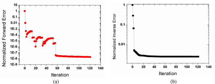
Convergence history of the PDE-constrained multispectral method with iteration: (a) forward error; (b) inverse error.

Fig. 3.

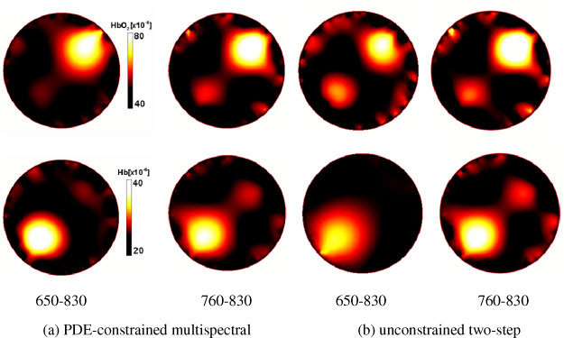
Images of reconstructed [HbO₂] (top row) and [Hb] (bottom row), obtained with the PDE-constrained multispectral and unconstrained two-step methods for two different wavelength sets.

As shown in Table 2, the PDE-constrained method leads to a significant saving in the CPU time in all cases. For the (650nm, 830nm) set, the PDE-constrained multispectral method reaches convergence in 14.5 min while the unconstrained two-step method takes about 168 min to converge at the same convergence criterion used in the PDE-constrained multispectral method. Therefore, the PDE-constrained multispectral method reduces the computation time by a factor of about 12. We observe a similar time saving in the other cases of a different wavelength set (see Table 2). The (760nm, 830nm) set data converges in 9.4 min using the PDE-constrained method and in 84 min using the unconstrained two-step method, respectively. Therefore, in this case, the PDE-constrained multispectral method accelerates the reconstruction process by a factor of about 10.

The main reason for this significant reduction in the CPU time can be explained by the fact that the PDE-constrained multispectral method does not require the exact solution of the forward problem at each iteration of optimization until it converges to the optimal solution, as mentioned earlier. Indeed we do not solve the forward problem for each wavelength, and instead we solve the linearized forward problem Eq. (12) which is much inexpensive to solve) for each wavelength. In other words, even a loose tolerance of 10⁻² can be used to solve for the linearized forward problem. Since we use a GMRES iterative solver, the usage of a loose tolerance (of 10⁻²) takes a much smaller number of iterations to a stopping criterion than the tight tolerance (of 10⁻¹⁰) used in the unconstrained two-step method. As a consequence, this leads to a significant time savings through the overall optimization process.

Figure 2(a) and 2(b) show the convergence history of the PDE-constrained multispectral method with the number of iterations. As expected, it is observed that the PDE-constrained multispectral scheme solves the forward and inverse problems simultaneously through decreasing all forward [Fig. 2(a)] and inverse [Fig. 2(b)] errors at once in each of optimization iterations.

Figure 3 shows the reconstructed concentration images of two chromophores HbO₂ and Hb obtained with two wavelength sets. Each row corresponds to the reconstructed images of HbO₂ and Hb concentrations, respectively, and the columns display the reconstructed images for wavelength sets 1 and 2, for the PDE-constrained and unconstrained two-step methods, respectively. In terms of image quality, the two methods with sets 1 and 2 give different results. For set 1, it can be seen from Table 2 and Fig. 3 that the PDE-constrained method gives more accurate results than the conventional method. The correlation factor of the PDE-constrained method is 0.62 and 0.71 for [HbO₂] and [Hb], respectively. This is almost 20% and 40% better than when the two-step method is used (ρ_c = 0.54 and 0.56, respectively). For set 2, both methods give similar results for both [HbO₂] and [Hb]. When both wavelength sets are compared against the method, the two-step method works better with the 760-830 set rather than the 650-830 set. On the other hand, the PDE-constrained method outperforms the unconstrained two-step method for both wavelength sets. In particular, it gives best results for the 650-830 set.

Also, we found that the two-step unconstrained method produces larger deviation factors due to overestimation or underestimation in either HbO₂ or Hb or both of the two (see Fig. 3). More evidences supporting this statement can be found from results obtained with the (760nm, 830nm) set. As compared to the results with the (650nm, 830nm) set, the two methods give lower accuracy both with respect to the correlation coefficient and the deviation factor as given in Table 2. Especially some cross-talk between two hemoglobin concentrations is observed in both of the two methods: the false Hb (HbO₂) perturbation is retrieved in the position of object 2 Eq. (1) where the medium has only inhomogeneity in HbO₂ (Hb). In addition to cross-talk, the conventional method reveals larger artifacts and overestimation or underestimation in both [HbO₂] and [Hb]. This nature of the (760nm, 830nm) set may be explained by the concept of a condition number κ(E) of the molar extinction coefficient matrix E of HbO₂ and Hb that represents a measure of how ‘well-posed’ a problem is: the larger κ(E) is, the more ‘ill-posed’ is the system. In other words, if the condition number is large, even a small error in the estimated absorption coefficient may cause a large error in the reconstructed hemoglobin concentration, and vice versa. In our cases, the condition numbers for the (650nm, 830nm) and (760nm, 830nm) sets are 1.76 and 3.17 respectively. Therefore it is evident that the (760nm, 830nm) set exhibits the nature of more ill-posed noise-sensitive problem, consequently making it more difficult to distinguish between the two unknowns, as compared to the (650nm, 830nm) set.

4.2 Experimental study

In addition to numerical studies, we have started to explore the code’s performance using experimental data obtained from tumor bearing mice. For this experiment 10⁶ cultured human Ewing sarcoma cells engineered to express luciferase (SK-NEP1-luc) were implanted intra-renally in NCR nude mice and allowed to grow until the tumor size reached about 1g as determined by weekly bioluminescence measurements. The experimental data was acquired with a continuous-wave digital optical tomography system that illuminates the target simultaneously with two wavelengths (λ = 760 nm and 830nm) modulated at 5 kHz and 7 kHz respectively. The system’s 16 sources and 32 detectors are configured in two rings, separated by 1.25cm, around a 3.175cm Delrin cylinder. Each ring contains 8 sources and 16 detectors arranged in a source-detector-detector-source configuration. The animal, anesthetized using isofluorane gas, was placed in the cylinder with the kidney and tumor located between the two rings of sources and detectors [see Fig. 4(a) ]. Then 1% Intralipid fluid was used to fill the remaining space in the cylinder to help reduce edge effects. The system uses silicon photodiodes to detect the transmitted and reflected photons passing through the cylinder. A digital-signal-processor (DSP) chip provides fast demodulation and control of the system giving an imaging frame rate of over 5 frames per second. More detailed information about the measurement system can be found elsewhere [18].

Fig. 4.

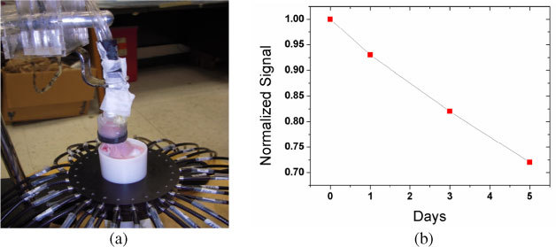
Optical imaging probe with mouse positioned in the cylinder (a) and signal changes observed over a 5 day period for the sum of all measurements (b).

To monitor the hemodynamic effects in the growing tumor, four sets of optical tomographic images (1000 frames of data - approximately three minutes of imaging) were obtained at days 0, 1, 3, and 5 after the tumor size was determined to have reached 1g. A 300-point subsection of the 1000 frames data with minimal motion was selected and averaged to remove any respiratory and other noise. After the data was acquired with the mouse in the cylinder a reference set of data was acquired for a homogeneous medium of 1% Intralipid.

Since the instrument used for this study does not provide absolute measurements due to the unknown calibration errors such as photon loss in fibers, we defined the following objective function [19]:

$$\varphi [{\text{HbO}}_{\text{2}}\text{,Hb}]=\frac{1}{2}{\displaystyle \sum _{\lambda }{\displaystyle \sum _s{\displaystyle \sum _d{\left|\frac{M_{\text{tar},s,d}^{\lambda }}{M_{\text{ref,}s,d}^{\lambda }}{P}_{\text{ref},s,d}^{\lambda }-P_{\text{tar},s,d}^{\lambda }\right|}^2}}}$$ (17)

where the subscripts s and d denote the numbers of sources and detectors. $M_{\text{tar},s,d}^{\lambda }$ and $M_{\text{ref,}s,d}^{\lambda }$ denote the spectral measurements at wavelength λ for the target medium of unknown optical properties and the reference medium of known optical properties, respectively. $P_{\text{ref},s,d}^{\lambda }$ and $P_{\text{ref},s,d}^{\lambda }$ are the corresponding forward predictions for the reference medium of known optical properties and the target medium of unknown optical properties, respectively. Here 1% Intralipid matching fluid is used as the reference medium.

Figure 4(b) shows the changes in measured signal intensity as it develops over the 5-day period when the experiments were performed. The value plotted as a function of time is the sum of measured optical signal for all source-detectors pairs, normalized by the sum of the day 0 signal. In general, we always saw a decline in signal intensity in almost all source detector pairs over time, which is caused by the continuous growth of the tumor, which is accompanied by a well-understood increased in vascularization (and hence blood volume) in the field of view [20,21].

Using data from all source-detector pairs we furthermore retrieved the three-dimensional spatial distributions of oxy- and deoxy-hemoglobin, (HbO₂) and (Hb) as well as their sum the total hemoglobin (THb). As with the numerical studies, we compare the performance of the two methods (PDE-constrained multispectral and conventional two-step methods) on the experimental data. We measure the CPU times of the two methods, and since the exact distributions of chromophores are not known for the mouse, we just provide a qualitative assessment of the results based on the expected biological change.

The reconstructed images of [THb], [HbO₂] and [Hb] are shown in Figs. 5 and 6 . Note that Figs. 5 and 6 show the results for the 2cmx3cmx3cm volume in the cylinder of height 8cm and diameter 3.175cm. We present here a drawing of the 3D volume contour of the reconstructed values above the given threshold, which can provide a better way for visual inspection of the time-trace results than the 2D cross-section maps. In terms of the CPU times, the PDE-constrained multispectral method took approximately 2 hrs to converge, while the conventional two-step method reached convergence in about 24 hours on a Dual Core Intel Xeon 3.33GHz processor: this constitutes acceleration factor of about 10. Furthermore, the two methods gave different trends of reconstructed chromophores over time. As can be seen in Fig. 5, the images generated by the PDE-constrained multispectral method clearly show that [HbO₂], [Hb], and [THb] increase in volume and value over time. This is expected as the tumor volume and vascular density increase over time as well [20,21]. This is also in agreement with the observed changes in optical signal shown in Fig. 4. On the other hand, this trend is not seen in the results obtained with the two-step method (Fig. 6). The [HbO₂] and [Hb] values decrease at 72 hrs and 5 days, respectively. We believe that this is an artifact introduced by the two-step method. Since the two-step method does not take any spectral constraints into account, it has been observed to produce less reliable results before [4,6,7] (e.g., artifacts, cross-talk and negative values).

Fig. 5.

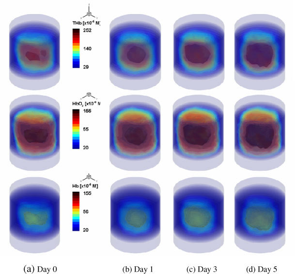
Reconstructed distributions of [THb] (1st row), [HbO₂](2nd row) and [Hb] (3rd row) as observed over the 5 day period, using the proposed PDE-constrained multispectral method, with a wavelength set of 760nm and 830 nm. Shown is the 2cmx3cmx3cm volume that includes a growing tumor in vivo.

Fig. 6.

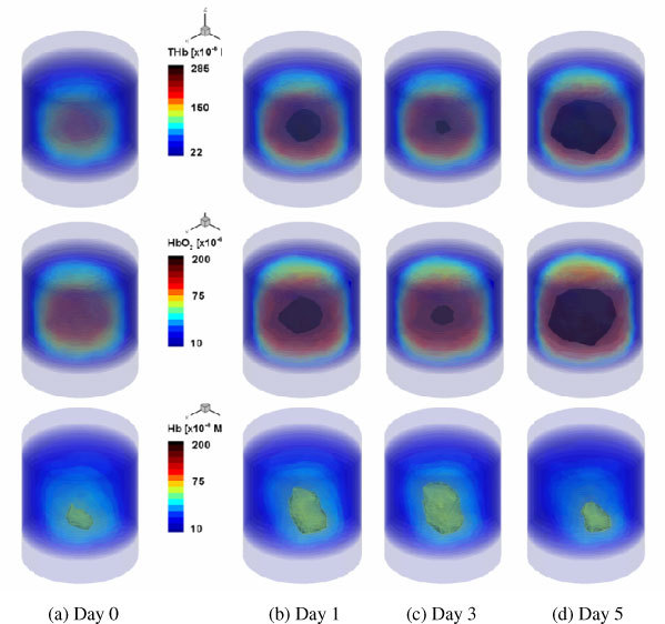
Reconstructed distributions of [THb](1st row), [HbO₂](2nd row) and [Hb](3rd row) over a 5-day period, using the conventional two-step method, with a wavelength set of 760nm and 830 nm. Shown is the 2cmx3cmx3cm volume that includes a growing tumor in vivo.

5. Conclusions

In this study, we present the first ERT-based PDE-constrained multispectral inverse method for direct imaging of chromophore concentrations in biological tissue. The proposed method is based on the reduced Hessian sequential quadratic programming method and solves the forward problem for each wavelength and the inverse problem for obtaining chromophore concentrations, in an all-at-once manner, which leads to a significant saving in the total image reconstruction time. We have evaluated the performance of the proposed algorithm through numerical studies and with experimental data obtained from tumor bearing mice.

We found that the PDE-constrained method not only reduces the image reconstruction time by a factor of up to 15 but also gives more accurate results as compared to the conventional two-step method. We also observed that the wavelengths pair (650 nm, 830 nm) produces more accurate results with less cross-talk than the wavelength pair (760 nm, 830 nm). The experimental results demonstrate that the PDE-constrained method gives reasonable results consistent with expected signal trends.