Complex Principal Components for Robust Motion Estimation

Abstract

Bias and variance errors in motion estimation result from electronic noise, decorrelation, aliasing, and inherent algorithm limitations. Unlike most error sources, decorrelation is coherent over time and has the same power spectrum as the signal. Thus, reducing decorrelation is impossible through frequency domain filtering or simple averaging and must be achieved through other methods.

In this paper, we present a novel motion estimator, termed the principal component displacement estimator (PCDE), which takes advantage of the signal separation capabilities of principal component analysis (PCA) to reject decorrelation and noise. Furthermore, PCDE only requires the computation of a single principal component, enabling computational speed that is on the same order of magnitude or faster than the commonly used Loupas algorithm. Unlike prior PCA strategies, PCDE uses complex data to generate motion estimates using only a single principal component. The use of complex echo data is critical because it allows for separation of signal components based on motion, which is revealed through phase changes of the complex principal components. PCDE operates on the assumption that the signal component of interest is also the most energetic component in an ensemble of echo data. This assumption holds in most clinical ultrasound environments. However, in environments where electronic noise SNR is less than 0 dB or in blood flow data for which the wall signal dominates the signal from blood flow, the calculation of more than one PC is required to obtain the signal of interest.

We simulated synthetic ultrasound data to assess the performance of PCDE over a wide range of imaging conditions and in the presence of decorrelation and additive noise. Under typical ultrasonic elasticity imaging conditions (0.98 signal correlation, 25 dB SNR, 1 sample shift), PCDE decreased estimation bias by more than 10% and standard deviation by more than 30% compared with the Loupas method and normalized cross-correlation with cosine fitting (NC CF). More modest gains were observed relative to spline-based time delay estimation (sTDE). PCDE was also tested on experimental elastography data. Compressions of approximately 1.5% were applied to a CIRS elastography phantom with embedded 10.4-mm-diameter lesions that had moduli contrasts of −9.2, −5.9, and 12.0 dB. The standard deviation of displacement estimates was reduced by at least 67% in homogeneous regions at 35 to 40 mm in depth with respect to estimates produced by Loupas, NC CF, and sTDE. Greater improvements in CNR and displacement standard deviation were observed at larger depths where speckle decorrelation and other noise sources were more significant.

I. Introduction

The determination of the time delay between two signals—one reference and one shifted—is a fundamental task in areas of research including medical imaging, radar, sonar, and speech processing. In medical ultrasound, motion estimation is performed in applications including phase aberration correction [1], [2], elastography [3]-[8], Doppler blood flow estimation [9], [10], and radiation force imaging [11]-[14]. In all of these applications, the physical principle underlying motion estimation is that changes in the path length between a group of acoustic scatterers and an ultrasound transducer will introduce a time delay in the backscattered ultrasound pulse. Along with fixed imaging parameters such as the center frequency and bandwidth, the performance of motion estimation is dependent upon the imaging environment. Signal correlation and SNR are especially important determinants of performance as expressed in the Cramer-Rao lower bound [15].

Motion estimators can be classified based upon the domain in which they operate. The most common phase domain techniques are the 1-D autocorrelator, developed by Kasai et al. [9], and the 2-D autocorrelator, developed by Loupas et al. [10]. Both techniques were developed to measure a single velocity estimate from an ensemble of echo data; however, they are also well suited to estimate pair-wise displacements, which can be combined to yield displacement profiles. The Loupas algorithm improved upon Kasai’s by accounting for local variations in the center frequency of the echo signal.

Although generally exhibiting a higher computational cost, several time-domain displacement estimators exhibit superior performance relative to Loupas [11], [13]. The spline-based time delay estimator (sTDE), developed by Viola and Walker, operates by forming a spline representation of the echo signal. The delay between a splined reference signal and a sampled shifted signal is located by minimizing an analytical mean squared error function.

Time-delay estimation performance can sometimes be improved by applying a pre-processing step using complex principal component filtering (PCF). With a computational cost comparable to a finite impulse response (FIR) filter, PCF was shown to reduce echo decorrelation and noise, thus reducing motion estimation errors [16]. Other PCA and blind source separation methods have been shown to improve performance in tissue classification, clutter rejection, physiological motion filtering, and radiation force induced displacement filtering [17]-[23]. Although PCA-based filtering techniques have been experimentally validated in a wide range of applications, there are limitations that include high computational complexity and the need for human input to select which PCs to retain and reject. PCDE utilizes complex echo data, which allows motion to be captured in a single principal component, as will be discussed subsequently. With the assumption that the signal component with the largest energy is also the signal component of interest, which is valid in most clinical ultrasound environments, PCDE can reduce or eliminate some of the limitations associated with other PCA-based techniques.

In this paper, we describe and characterize a novel estimator technique, termed the principal component displacement estimator (PCDE). This technique combines the decorrelation reduction of PCF with the modest computational cost of phase-domain estimators and the high performance of time-domain techniques. PCDE is compared against the Loupas algorithm, sTDE, and normalized cross correlation with cosine fitting (NC CF).

II. Methods

A. Principal Component Displacement Estimation (PCDE)

PCDE operates on an ensemble of complex data sampled in both range and pulse number. Complex data can be formed via hardware or software demodulation, including Hilbert transformation of RF data. The complex principal components of the data matrix, X, are determined using the covariance method of principal component analysis [24]. To illustrate this technique, first consider the matrix of complex echo data X, with T observations (samples through depth) and N variables (A-lines). The matrix X is mean-reduced so that each column in X has zero mean. The sample autocorrelation matrix, R̂ is computed by

$$\widehat{R}=X^{\ast }X,$$ (1)

where X* is the conjugate transpose of X. The complex PCs are then found by performing an eigenvalue decomposition to diagonalize R̂:

$$V^{-1}\widehat{R}V=\mathrm{\Lambda },$$ (2)

where V is a matrix with eigenvectors arranged in columns. Although the precise definition of what are considered to be the PCs of X has varied between different authors, a common notation is to define the PCs as the eigenvectors of the autocorrelation matrix or the eigenvectors weighted by the corresponding eigenvalues [24]. In this paper, we will define the PCs as the eigenvectors of the autocorrelation matrix. Therefore, the first complex PC of X, υ₁, is defined as the first column of V. The estimate of time delays through ensemble length, Δτ̂ [samples] (with dimensions N × 1), are calculated from υ₁ using

$$\mathrm{\Delta }\widehat{\tau }=\frac{{\tan }^{-1}\left\{\frac{\mathrm{Im}({\upsilon }_1)}{\mathrm{Re}({\upsilon }_1)}\right\}}{{\tan }^{-1}\left\{\frac{\mathrm{Im}\left[{\sum }_{m=0}^{M-2}{\sum }_{n=0}^{N-1}X\ast (m,n)X(m+1,n)\right]}{\mathrm{Re}\left[{\sum }_{m=0}^{M-2}{\sum }_{n=0}^{N-1}X\ast (m,n)X(m+1,n)\right]}\right\}}.$$ (3)

The numerator of (3) represents the phase of the first principal component, whereas the denominator is an estimate of the local center frequency via the lag-1 autocorrelation of the ensemble. Note the similarity to Loupas’ algorithm, with the first PC being used instead of the signal autocorrelation (we discuss the relationship between the two algorithms in Section IV-E).

Fig. 1 illustrates the signal separation capabilities of PCDE when operating on an ensemble of echo data. Fig. 1(a) shows multiple signal components with different motion characteristics, which are summed and weighted according to their relative positions within the point spread function (psf) of the acoustic beam (i.e., w₁ > w₂ > w₃). Differential motion within the acoustic beam is a major source of estimation bias and variance errors, which are particularly common in elasticity imaging [14], [25]. Although sources of electronic noise can be partially eliminated using conventional frequency-domain filtering, decorrelation sources have spectra that overlap with the signal of interest [s₁(t) from Fig. 1]. Thus, averaging or filtering in the frequency domain cannot reject undesirable signal components, yielding corrupted motion estimates. In contrast, PCDE operates in the time domain where it is possible to separate signals of overlapping spectra.

Fig. 1.

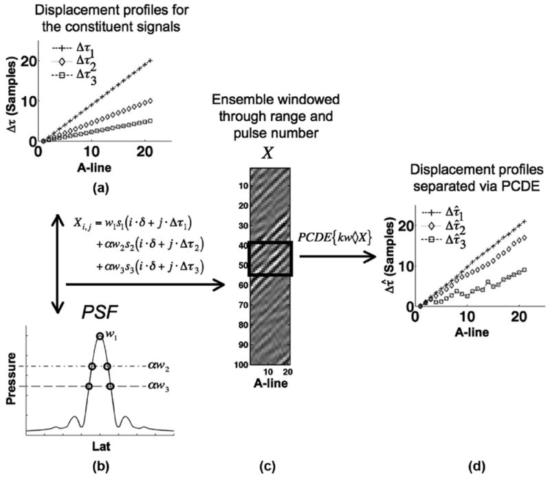
Three source signals with variable delay characteristics (panel A) and weightings (panel B) are summed to form a simulated ensemble of echo data, X, (panel C) which models decorrelation arising from differential motion across the point spread function (psf). Resulting echo data, X, is windowed, kw◇ X as denoted by the rectangle. PCDE operates on this subset of echo data to compute principal components (PCs), which correspond to different source signals. In panel D, the PCDE estimated displacements of the sources signals, Δτ̂, are illustrated. In this paper, we are only concerned with the most energetic source signal and so only the first PC was computed.

An example of simulated RF data resulting from the mixing of three signal components is shown in Fig. 1(b). After processing with PCDE, the mixed signals are separated from the ensemble data. This enables motion estimation on the desired signal component, s₁(t). Time delay estimates can also be performed on secondary signal components, s₂(t) and s₃(t) [Fig. 1(c)].

B. Sources of Decorrelation and Simulation Signal Model

As predicted by the Cramer-Rao lower bound for displacement estimation [15], decorrelation is a major limiter of motion estimation performance. In this paper, we define two types of decorrelation based upon their respective physical sources.

One source of decorrelation arises from new acoustic targets moving into and out of the acoustic beam. This type of decorrelation is most significant in applications with large displacements such as elastography and blood flow estimation. In this paper, we refer to this type of decorrelation as out-of-beam decorrelation because the underlying acoustic scatterers move out of the acoustic beam through time. We model this type of decorrelation in our simulations by specifying a correlation value and using Cholesky factorization to add new, uncorrelated signal components [11], [26]. This method operates by first forming a 2 × 2 symmetric matrix, A, which is composed of ones along the diagonal entries and the desired correlation coefficient, ρ along the off-diagonals. Using Cholesky factorization, matrix A is then factored into the product of an upper triangular matrix, Q and its transpose: A = Q′ Q. The upper right and lower right entries of Q are then used to weight the initial signal, c₁(t) and another uncorrelated signal of the same power spectrum, c₂(t). The output signal, s(t) is then formed by summing the signal components c₁(t) and c₂(t) and weighting them by the upper right and lower right entries of the Cholesky factorized matrix, Q₁₂ and Q₂₂ respectively:

$$s(t)=Q_{12}{c}_1(t)+Q_{22}{c}_2(t).$$ (4)

The signal component c₂(t) represents new acoustic scatterers moving into the acoustic beam, and thus, the source of out-of-beam decorrelation. As a result of this method, the output signal, s(t) is constructed so that it has a predefined correlation coefficient of ρ with the initial signal, c₁(t).

Another type of decorrelation, which is illustrated in Fig. 1, originates from differential displacements within the psf. This source of decorrelation is fundamentally different from out-of-beam decorrelation because the acoustic targets do not necessarily leave or enter the acoustic beam—they only exhibit differential axial displacement with respect to one another. Accordingly, we refer to this type as differential motion decorrelation. Differential motion decorrelation can be associated with what in other contexts is referred to as axial shear. Although many motion estimation applications are subject to differential motion within the psf, acoustic radiation force imaging applications are especially susceptible. Several studies have indicated that this is a major source of motion estimation corruption [14], [25].

To model differential motion decorrelation, three independent source signals s_l(t), representing echoes from scatterers at different locations within the psf, were weighted and summed to form the simulated ensemble, X_i,j:

$$X_{i,j}=w_1{s}_1(i·\delta +j·\mathrm{\Delta }{\tau }_1)+\alpha w_2{s}_2(i·\delta +j·\mathrm{\Delta }{\tau }_2)+\alpha w_3{s}_3(i·\delta +j·\mathrm{\Delta }{\tau }_3)$$ (5)

$$s_l(i·\delta +j·\mathrm{\Delta }{\tau }_l)=Q_{12}{c}_{l,1}(i·\delta +j·\mathrm{\Delta }{\tau }_l)+Q_{22}{c}_{l,2}(i·\delta +j·\mathrm{\Delta }{\tau }_l),$$ (6)

where δ is the sampling interval in range, Δτ_l are transmit to transmit time shifts, w_l are weighting coefficients corresponding to the source scatterers’ relative position in the psf, and α is a parameter that is varied in simulation to reduce or intensify decorrelation originating from differential motion. Eq. (6) is a discrete formulation of (4) describing the Cholesky factorization method for simulating out-of-beam decorrelation. This method is applied to each s_l(t) individually before summation in (5). Each echo signal s_l(t) is formed by summing two uncorrelated signal components, c_l,1(t) and c_l,2(t). These signal components are weighted by coefficients Q₁₂ and Q₂₂, which are determined by Cholesky factorization as described previously. The ratio of β₁ to β₂ determines the out-of-beam correlation of s_l(t) through time. In practice, differential motion decorrelation may vary because of non-uniform mechanical properties across the psf and because of changes in the f-numbers of the pushing and tracking beams [14].

C. Simulation Methods

Synthetic ultrasound data was generated in MATLAB (MathWorks Inc., Natick, MA). A-lines were formed by convolving the acoustic targets, modeled as Gaussian white noise, with the psf of the ultrasound pulse, which was represented as a sinusoid with a Gaussian envelope:

$$\mathrm{psf}(t)=e^{-(t^2/(2\sigma ))}\sin (2\pi f_{0}t)$$ (7)

$$\sigma =\frac{0.42466}{{\mathit{Bf}}_0},$$ (8)

where B is fractional bandwidth, f₀ is center frequency, and 0.42466 relates the full-width at half-maximum value of a Gaussian to its standard deviation.

To produce known subsample or sample delays between a reference and delayed echo signal, simulated data was generated at a sampling rate 40 times the rate desired for analysis. These signals were then downsampled starting at different samples to produce reference and delayed signals with a known subsample delay. Independent Gaussian-distributed white noise records were added to the reference and shifted signals to produce a desired SNR. Out-of beam and differential motion decorrelation were introduced to test the robustness of the various algorithms. Default simulation parameters are listed in Table I.

TABLE I.

Default Simulation Parameters.

Parameter	Value
Center frequency (f0)	8 MHz
Sampling frequency (fs)	40 Mhz
Signal to noise ratio (SNR)	25 dB
Fractional bandwidth (BW)	50%
Kernel length	3 periods
Out-of-beam correlation (ρ)	0.98
Differential motion weighting (α)	1
Differential motion parameters	Value
Δτ1 : Δτ2 : Δτ3	1: 1/2 : 1/4 samples
w1 : w2 : w3	$1:1/\sqrt{2}:1/2\mathrm{samples}$

D. Elastography Experiments

Experiments were performed on a CIRS Model 049A Elasticity QA phantom (Norfolk, VA ) with 10.4-mm-diameter cylindrical lesions located at 30 mm in depth. Three lesion types, with elasticity values ranging between 8.7 and 100 kPa embedded in a 25.2 ± 4 kPa homogeneous background, were imaged. Elasticity values for each lesion type with standard deviations, as provided by the manufacturer data sheet, are provided in Table II. The phantom was compressed with a motion controller attached to a Philips 15–6L compact linear array transducer (Philips Healthcare, Andover, MA), which operated at approximately 5.5 MHz center frequency. RF data frames were acquired after incremental compressions of 50 μm for 10 frames following the multi-compression elastography technique described in Lu et al. [5], [27]. This compression technique resulted in approximately 1.5% compression in regions of the 25.2 kPa background. RF data was obtained using an Ultrasonix RP scanner (Ultrasonix, Vancouver, BC, Canada). Displacements were computed off-line using a 3-period kernel window, and for sTDE and NC CF techniques, a 5-period search window. Strains were rendered from the displacement data at frame 10 using a Gaussian staggered strain filter with a full-width at half-maximum of 1.5 mm [28]. The staggered strain filter was equivalent to a Gaussian low-pass filter of the displacement data followed by differentiation along the range dimension using a filter convolution template [29]: [1 −1]^T. A summary of experimental parameters is listed in Table III.

TABLE II.

Elastography Phantom Stiffness.

Lesion type	Elasticity (kPa)
Type I	8.7 ± 3
Type II	12.8 ± 4
Type III	100 ± 10
Background	25.2 ± 4

TABLE III.

Elastography Parameters.

Parameter	Value
Center frequency (f0)	5.5 MHz
Sampling frequency (fs)	40 MHz
Fractional bandwidth (BW)	50%
Kernel window length	3 periods or 432 μm
Search window length	5 periods or 674 μm
Kernel window overlap	90%
Median filtering	None
Staggered strain filter width	1.5 mm

Performance of the proposed algorithms was assessed using two metrics: contrast-to-noise ratio (CNR) and displacement standard deviation. Using either metric, performance varied significantly with depth. Standard deviation measurements were larger at greater depths. Likewise, CNR values were lower if the background region was placed below, rather than above, the lesion. To illustrate this trend, we report standard deviation and CNR values at two representative depths 20 mm apart.

To compute CNR, a circular region of interest (ROI) with a 5 mm diameter, approximately half the diameter of the lesion, was selected inside the lesion and two ROIs were selected outside the lesion. The two background regions were located diagonal to the lesion and centered at 20 and 40 mm in range. The location of the outside ROIs was selected diagonal to the lesion, rather than directly above or below, to reduce the impact of stress concentration artifacts on CNR calculations as discussed in Varghese and Ophir [30]. Fig. 3 illustrates the regions used to compute a CNR for each strain image using the following expression [31]:

$$\mathrm{CNR}=\frac{\left|{\mu }_t-{\mu }_b\right|}{\sqrt{{\sigma }_t^2+{\sigma }_b^2}/2},$$ (9)

where μ is the mean strain value and σ is the standard deviation of strain values within the ROI of the target or background.

Fig. 3.

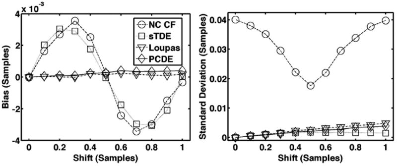
Average bias (left) and standard deviation (right) for each estimator over 1000 trials when subsample shifts are varied and the signal model does not include electronic noise or decorrelation.

Measures of displacement standard deviation were computed over regions spanning 15 to 20 mm and 35 to 40 mm in depth following the methods of Du et al. [5]. Briefly, to reduce the variations in displacement through depth, the mean displacement over depth was subtracted from the data by fitting the data to a line. Nonstationarities in the lateral direction remained because of small irregularities from sources such as phantom heterogeneity and non-uniform boundary effects, so the displacement was fit in the lateral dimension to a fourth-order polynomial. This function was then subtracted from the data and standard deviations were computed from this compensated region of displacement estimates.

III. Results

A. Effects of Decorrelation on Motion Estimation Performance

Fig. 3 shows average bias and standard deviation over 1000 trials for PCDE, Loupas, sTDE, and NC CF in the absence of noise, out-of-beam decorrelation, and differential motion decorrelation. All other simulation parameters were set according to the default values listed in Table I. Although no real application will be absent noise and decorrelation, this scenario highlights intrinsic limitations in the algorithms.

Figs. 4 and 5 illustrate estimator performance with either out-of-beam or differential motion decorrelation. Row A of Fig. 4 illustrates bias and standard deviation when only out-of-beam decorrelation is simulated (α = 0), whereas row B includes differential motion decorrelation (α = 1). Underestimation of the true displacement is more pronounced in row B, where multiple source signals are included in the signal model. Row A of Fig. 5 illustrates estimator performance when only differential motion decorrelation is simulated (ρ = 1.0), whereas row B includes out-of-beam decorrelation (ρ = 0.98).

Fig. 4.

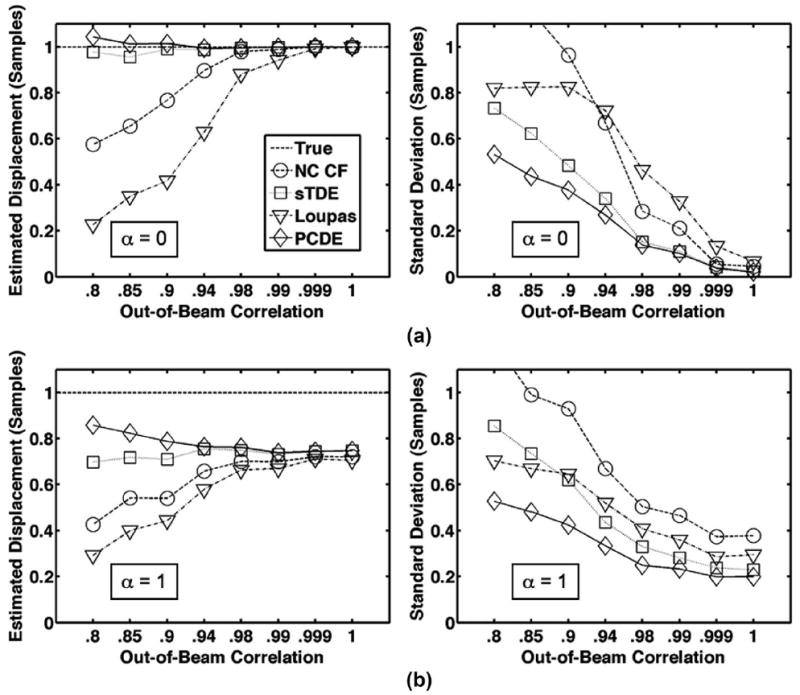
Row (a) illustrates average estimated displacement (left) and standard deviation (right) for each estimator over 1000 trials when only out-of-beam decorrelation is simulated and differential motion is not present (α = 0). Resulting echo correlation was varied between 0.8 and 1.0. In row (b), average estimated displacement (left) and standard deviation (right) are illustrated when both out-of-beam decorrelation and differential motion decorrelation are simulated. Differential motion weighting was set according to default parameters in Table I (α = 1). The dashed line is defined as the ‘true’ displacement, which corresponds to the peak displacement in the beam. For illustrative purposes, the x-axis is not a linear scale.

Fig. 5.

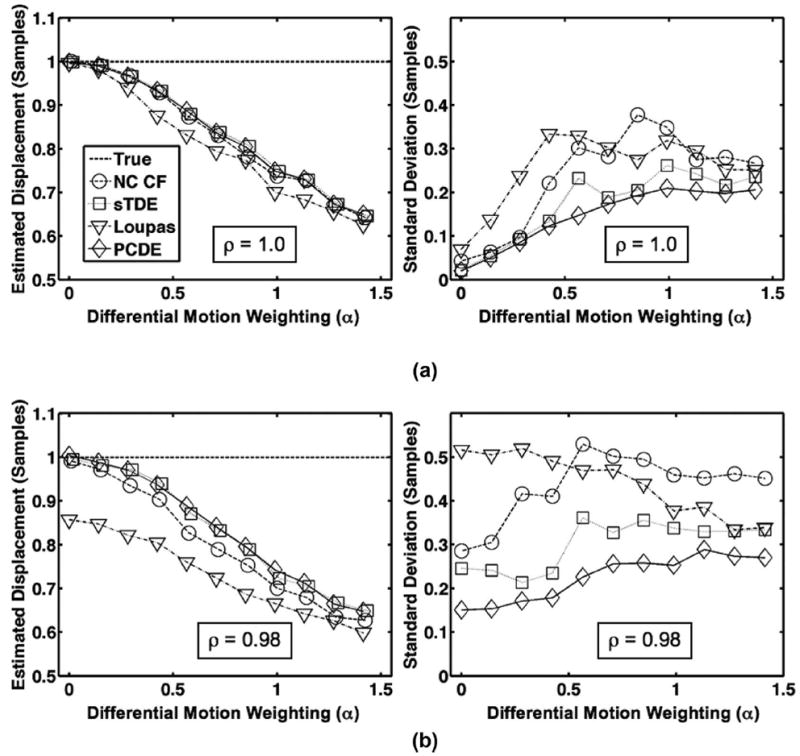
Row (a) illustrates average estimated displacement (left) and standard deviation (right) for each estimator over 1000 trials when only differential motion decorrelation is simulated with no out-of-beam decorrelation (ρ = 1.0). In row (b), average estimated displacement (left) and standard deviation (right) for each estimator over 1000 trials are illustrated when both out-of-beam decorrelation and differential motion decorrelation are simulated. The dashed line is defined as the ‘true’ displacement, which corresponds to the peak displacement in the beam. Echo correlation resulting from out-of-beam decorrelation was set according to default parameters in Table I (ρ = 0.98). In all cases, the differential motion weighting coefficient was varied between 0 and $\sqrt{2}$.

B. Effects of Displacement, SNR, Fractional Bandwidth, and Window Length on Motion Estimation Performance

Simulations were performed with default parameters listed in Table I, including both out-of-beam decorrelation (ρ = 0.98) and differential motion decorrelation (α = 1). Results are displayed in Figs. 6-10 to illustrate estimator performance as a function of subsample shifts (Fig. 6), shifts between 1 and 3 samples (Fig. 7), SNR (Fig. 8), fractional bandwidth (Fig. 9), and kernel window length (Fig. 10).

Fig. 6.

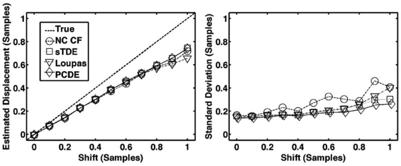
Average estimated displacement (left) and standard deviation (right) for each estimator over 1000 trials when subsample shift is varied between 0 and 1 sample. The dashed line is defined as the ‘true’ displacement, which corresponds to the peak displacement in the beam. The default simulation conditions of Table I were used such that both out-of-beam decorrelation and differential motion decorrelation were simulated.

Fig. 10.

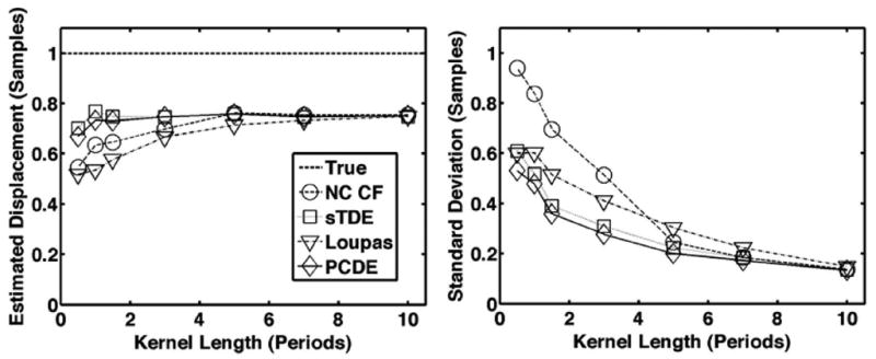
Average estimated displacement (left) and standard deviation (right) for each estimator over 1000 trials when kernel length is varied between 0.5 and 10 periods. The dashed line is defined as the ‘true’ displacement, which corresponds to the peak displacement in the beam. The default simulation conditions of Table I were used such that both out-of-beam decorrelation and differential motion decorrelation were simulated.

Fig. 7.

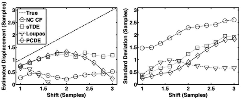
Average estimated displacement (left) and standard deviation (right) for each estimator over 1000 trials when simulated echo shifts are varied between 1 and 3 samples. The dashed line is defined as the ‘true’ displacement, which corresponds to the peak displacement in the beam. The default simulation conditions of Table I were used such that both out-of-beam decorrelation and differential motion decorrelation were simulated.

Fig. 8.

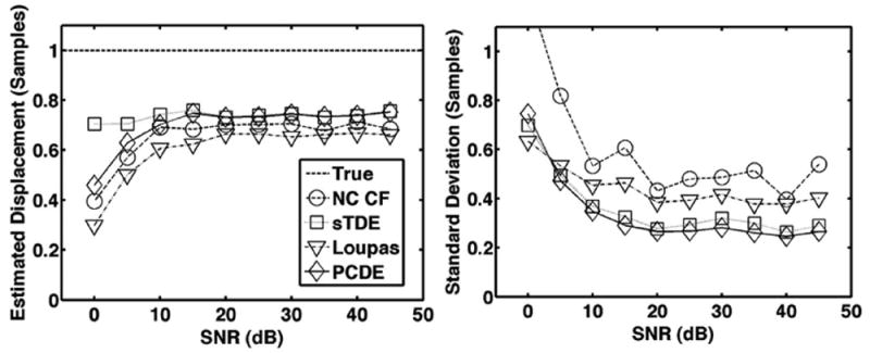
Average estimated displacement (left) and standard deviation (right) for each estimator over 1000 trials when simulated SNR is varied between 0 and 45 dB. The dashed line is defined as the ‘true’ displacement, which corresponds to the peak displacement in the beam. The default simulation conditions of Table I were used such that both out-of-beam decorrelation and differential motion decorrelation were simulated.

Fig. 9.

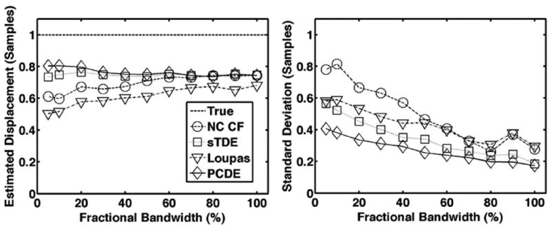
Average estimated displacement (left) and standard deviation (right) for each estimator over 1000 trials when fractional bandwidth is varied between 5% and 100%. The dashed line is defined as the ‘true’ displacement, which corresponds to the peak displacement in the beam. The default simulation conditions of Table I were used such that both out-of-beam decorrelation and differential motion decorrelation were simulated.

C. Motion Estimation Performance in Elastography Imaging

Displacement maps were rendered from each motion estimator using a 3-period kernel window with 90% overlap. Example displacement maps of lesion type I are depicted in Fig. 11. Displacement corruption is noticeably worse with increased depth, where noise and decorrelation was more prevalent because of attenuation of signal amplitude and greater out-of-beam motion.

Fig. 11.

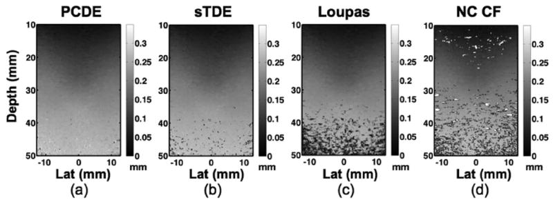
Experimental elastography displacement maps formed using a) principal component displacement estimation, b) spline time delay estimation (sTDE), c) the Loupas algorithm, and d) normalized cross-correlation with cosine fitting (NC CF). Experiments used a CIRS Model 049A phantom with type I lesion of approximately 8.7 kPa and background stiffness of approximately 25.2 kPa.

Displacement maps were computed in homogeneous regions of the 25.2 kPa background and average displacement standard deviation was computed for two depths: 15 to 20 mm and 35 to 40 mm. Average displacement standard deviation over nine trials for each region and each motion estimator are listed in Table IV. Standard deviation was estimated for each region as described in Section II-D. The lateral extent of each region was approximately 25.6 mm.

TABLE IV.

Elastography Displacement Standard Deviation.

Algorithm	15 to 20 mm STD (μm)	35 to 40 mm STD (μm)
PCDE	4.21	13.1
Spline TDE	4.47	39.8
Loupas	4.20	84.5
NC CF	89.1	152

Images of strain, from approximately 0 to 1.5%, are illustrated in Fig. 12 for each motion estimator (columns) and for lesion type I (row A), lesion type II (row B), and lesion type III (row C). Elastograms were produced from the displacement data by applying a Gaussian staggered strain linear filter with a 1.5 mm full-width at half-maximum. Performance of each algorithm is quantified via CNR calculations using (9) when background ROIs were centered at 20 mm [Fig. 13(a)] and 40 mm [Fig. 13(b)].

Fig. 12.

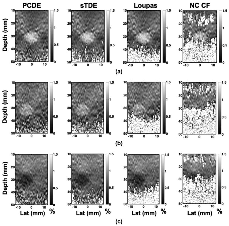
Elastograms formed using principal component displacement estimation (column I), spline time delay estimation (column II), the Loupas algorithm (column III), and normalized cross-correlation with cosine fitting (column IV). Rows are elastograms of lesion type I (row aA), lesion type II (row b), and lesion type III (row c). In all instances, kernel length was 3 periods with 90% overlap.

Fig. 13.

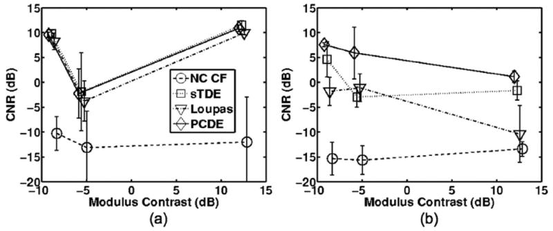
Average contrast to noise ratio (CNR) values when the background region is centered at a) 20 mm and b) 40 mm. Error bars illustrate the mean CNR plus or minus one standard deviation over 3 trials.

IV. Discussion

A. Computational Cost of PCDE

Computational time is an important feature of motion estimation algorithms as it is generally desirable to apply them to real-time applications. The computational cost of PCDE is dramatically lower than sTDE and is very competitive with the Loupas method, depending on the length of the ensemble. Although eigenvalue decomposition is computationally expensive, PCDE only requires calculating the first PC, which can potentially be reduced to an O(N) computation [32]. As implemented in this paper, PCDE used the eigs function in MATLAB to capture only the first PC from a symmetric autocorrelation matrix.

The time required for each algorithm to compute a displacement profile in MATLAB was averaged over 1000 trials and is reported in Fig. 14. Results are shown as a function of ensemble length. Two variations of PCDE are implemented. Although estimation performance was equivalent, there was a dramatic difference in computation time when eigenvalues were computed with the MATLAB eigs function versus the eig function. The eigs function uses routines from Fortran libraries that are better suited for large sparse matrices, whereas eig uses routines that are better suited for small, non-sparse matrices. Our simulations show that at a 3-period kernel window length, the eig function is much more efficient with small ensemble lengths, less than 75 A-lines; eigs becomes more efficient at ensemble lengths greater than 75.

Fig. 14.

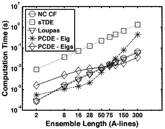
Time to compute one displacement profile averaged over 1000 trials. Ensemble lengths are varied between 2 and 300 A-lines. ‘PCDE – Eig’ denotes PCDE estimates when MATLAB function ‘eig’ is used to compute eigenvectors. Similarly, ‘PCDE – Eigs’ denotes PCDE estimates when MATLAB function ‘eigs’ is used to compute eigenvectors.

As anticipated, PCDE was more than an order of magnitude faster than sTDE but slightly slower than the Loupas algorithm at ensemble lengths less than 4 A-lines using the eig command. Conclusions from these results are limited because they were performed in MATLAB, which is more highly optimized for certain operations. Although PCDE showed computational times on the same order of magnitude or faster than Loupas in this setting, it is anticipated that the computational complexity of PCDE can be reduced with further optimization of the algorithm.

B. PCDE in Simulation

Fig. 3 shows bias and standard deviation for motion estimates performed on simulated echoes under ideal conditions, which did not include electronic noise or decorrelation. The periodic trends in the bias of sTDE and NC CF, and the constant growth in bias from Loupas agree well with past studies [11]-[13].

Simulation results from Figs. 4 and 5 illustrate that PCDE is more robust to decorrelation than other commonly used estimators. Whether out-of-beam or differential motion decorrelation were simulated alone [Figs. 4(a) and 5(a)] or together [Figs. 4(b) and 5(b)], PCDE exhibited lower bias and standard deviation across a wide range of decorrelation levels. PCDE performance was most superior at higher levels of decorrelation (lower out-of beam correlation or higher weighting coefficient, α). In agreement with past literature [14], [25], a negative bias with respect to the true displacement is most prevalent in cases where differential motion decorrelation exists. Differential motion decorrelation was absent in Figs. 3 and 4(a).

Results from Figs. 6-10 illustrate that PCDE exhibits lower bias and standard deviation than NC CF and the Loupas method over a wide range of simulation parameters. PCDE superiority over Loupas is especially apparent at larger displacements such as in Fig. 7. This is likely because of the susceptibility of Loupas to aliasing, which occurs when displacement between consecutive A-lines is greater than half the wavelength. Although PCDE also breaks down at large displacements because of aliasing, our simulation results show that PCDE is more robust than Loupas, with performance similar to sTDE in terms of bias and better than sTDE in terms of standard deviation. Additional simulation results show that PCDE is robust to several error sources and limitations including random noise (Fig. 8), low fractional bandwidth (Fig. 9), and short kernel window lengths (Fig. 10). The only condition under which Loupas exhibited slightly better performance was at 0 dB SNR. Although PCDE bias was lower than Loupas, the standard deviation of PCDE was slightly higher. Because PCDE relies on the signal of interest exhibiting the greatest energy, it is likely that noise was introduced into the first PC at 0 dB and some of the desired signal was pushed into the second PC, thus resulting in poorer performance.

C. Elasticity Imaging With PCDE

PCDE was applied to experimental multi-compression elastography data to illustrate its performance when decorrelation and other noise sources limit performance. Displacement data shown in Fig. 11 illustrates a dramatic reduction in decorrelation artifacts with PCDE when the type I elastography lesion was imaged. Decorrelation artifacts are particularly apparent at larger depths. At more shallow depths where displacement is smaller and SNR and correlation are expected to be high, performance of the techniques was more similar, in agreement with simulation results.

The standard deviation of displacement estimates at regions between 15 to 20 mm and 35 to 40 mm are reported in Table IV. PCDE, sTDE, and Loupas exhibited similar performance at the 15 to 20 mm depth, as anticipated. However, at 35 to 40 mm, where noise and decorrelation were more prevalent, PCDE vastly outperformed rival techniques with a reduction in standard deviation of at least 67%.

Similar trends are visualized in the elastograms of Fig. 12, where decorrelation artifacts are reduced in the PCDE image. In general, PCDE exhibited the fewest artifacts, followed by sTDE, Loupas, and NC CF. Typically, cross-correlation techniques, such as NC CF, have been used as one-dimensional displacement estimators in elastography [5], [6]. As is apparent in Fig. 12, at kernel lengths around 3 periods, performance of NC CF is poor and larger kernel lengths are necessary. Larger kernel lengths, however, degrade resolution and increase computational time. Thus, the results from Figs. 12-14 indicate that PCDE achieves better imaging performance, in terms of SNR and CNR, with better resolution and lower computational cost than alternative motion estimators examined in this paper.

Image quality is quantified in Fig. 13 and confirms the general trends of the elastography images of Fig. 12. When the background region was centered at 20 mm (b₁ in Fig. 2), CNR was similar among the displacement estimators. When the background region was placed at 40 mm (b₂ in Fig. 2), CNR calculations showed superior performance for PCDE as compared with sTDE, Loupas, or NC CF. Fig. 13(b) illustrates average CNR improvements from PCDE that were at least 2.9 dB and as much as 6.9 dB over other estimators.

Fig. 2.

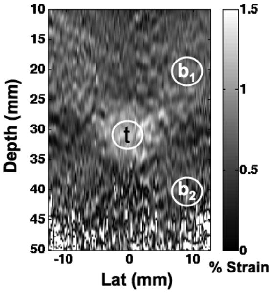
Regions of interest used to compute contrast to noise ratio (CNR) from elastograms. The target region, t was used along with a background region that was centered at either 20 mm in depth, b₁, or centered at 40 mm in depth, b₂. Regions of interest were approximately 5 mm in diameter.

D. The Significance of Complex Principal Components

The use of complex echo data are critical because it allows the motion of the signal component of interest to be captured in a single principal component. This capability can only be achieved using complex echo data because motion is revealed through phase changes, which appear as complex weightings of the same principal component.

PCDE uses complex echo data with principal component analysis to differentiate desirable from undesirable signal sources. This separation technique works under the assumption that the signal component with the most energy is also the most desirable. As illustrated in Fig. 8, this assumption holds until 0 dB SNR, which is below the SNR levels seen in medical ultrasound applications, with the possible exception of blood flow estimation. Moreover, in blood flow estimation there is often a spatial overlap of signal from the vessel wall, called clutter, which dominates the desired blood flow signal. Without a separate clutter filtering step, our assumption in this environment would be invalid because the signal of interest, blood flow, would have a lower energy than the clutter signal.

E. The Relationship to Phase-Based Estimators

The Kasai and Loupas phase domain-based motion estimators have been widely used in blood flow and other applications [9], [10], [12]. These techniques compute an estimate of the lag-1 autocorrelation from an ensemble of echo data. In contrast to Kasai, the Loupas algorithm computes a lag-1 autocorrelation estimate in both dimensions, so that the local center frequency is estimated. The velocity estimate determined by both techniques is derived from the phase of the autocorrelation estimate. In a related manner, PCDE computes a matrix of autocorrelation estimates. The main diagonal is the lag-0 estimate, the first off-diagonal entries represent estimates of lag-1 autocorrelation, the second off-diagonal entries represent lag-2 estimates, and so on. Thus, rather than computing an average lag-1 autocorrelation estimate, PCDE incorporates all possible lag-N autocorrelation estimates from the ensemble of echo data and then identifies the eigenvectors of the symmetric autocorrelation matrix.

V. Conclusions

We have presented a novel motion estimator termed the principal component displacement estimator (PCDE). Across a broad range of simulations incorporating decorrelation and noise, PCDE exhibited more accurate and precise displacement estimates than the Loupas algorithm and normalized cross-correlation with cosine fitting. Under most conditions, PCDE outperformed spline-based time delay estimation while showing significant reductions in computation time in MATLAB. Elastography images were formed using PCDE-derived displacements and compared against other techniques. PCDE reduced decorrelation artifacts and improved image quality in terms of displacement standard deviation and image CNR. These data illustrate that PCDE is accurate and robust with modest computational cost, making it a superior approach for many real-time imaging applications.

Biographies

F. William Mauldin, Jr. earned a B.S. degree in applied science from the University of North Carolina at Chapel Hill in 2007. He is currently a Ph.D. candidate in biomedical engineering at the University of Virginia. His research interests include adaptive signal filtering, time-delay estimation, and acoustic radiation force imaging.

Francesco Viola holds an Italian Laurea in biomedical engineering from the Polytechnic University of Milan, Milan, Italy, and a Ph.D. in biomedical engineering from the University of Virginia, Charlottesville, VA . He currently serves as Vice President of Engineering and Technology at HemoSonics LLC, a medical device start-up that he co-founded to develop and bring to market novel diagnostics for the characterization and monitoring of hemostasis. Dr. Viola also has an appointment as Visiting Research Professor within the Department of Biomedical Engineering at the University of Virginia. His research interests include ultrasound beamforming, tissue elasticity estimation, acoustic radiation force imaging, and time-delay estimation.

William F. Walker received the B.S.E. and Ph.D. degrees in 1990 and 1995, respectively, from Duke University, Durham, NC. His dissertation explored fundamental limits on the accuracy of adaptive ultrasound imaging.

After completing his doctoral work, he stayed on at Duke as an assistant research professor in the Department of Biomedical Engineering. At the same time, he served as a senior scientist and president of NovaSon Corporation located in Durham, NC. In 1997, he joined the faculty of the Department of Biomedical Engineering at the University of Virginia, being promoted to associate professor in 2003. He is an active founder in two ultrasound-based startup companies, PocketSonics Inc. and HemoSonics LLC. His research interests include aperture domain processing, beamforming, angular scatter imaging, tissue elasticity imaging, low-cost system architectures, blood coagulation, and time delay and motion estimation.

References

- 1.Trahey GE, Nock LF. Synthetic receive aperture imaging with phase correction for motion and for tissue inhomogeneities—Part II: Effects of and correction for motion. IEEE Trans Ultrason Ferroelectr Freq Control. 1992;39(4):496–501. doi: 10.1109/58.148540. [DOI] [PubMed] [Google Scholar]
- 2.Ng GC, Worrell SS, Freiburger PD, Trahey GE. A comparative evaluation of several algorithms for phase aberration correction. IEEE Trans Ultrason Ferroelectr Freq Control. 1994;41(5):631–643. [Google Scholar]
- 3.O’Donnell M, Skovoroda AR, Shapo BM, Emelianov SY. Internal displacement and strain imaging using ultrasonic speckle tracking. IEEE Trans Ultrason Ferroelectr Freq Control. 1994;41(3):314–325. [Google Scholar]
- 4.Ophir J, Alam SK, Garra B, Kallel F, Konofagou E, Krouskop T, Varghese T. Elastography: Ultrasonic estimation and imaging of the elastic properties of tissues. Proc Inst Mech Eng. 1999;213(pt H):203–233. doi: 10.1243/0954411991534933. [DOI] [PubMed] [Google Scholar]
- 5.Du H, Liu J, Pellot-Barakat C, Insana MF. Optimizing multicompression approaches to elasticity imaging. IEEE Trans Ultrason Ferroelectr Freq Control. 2006;53(1):90–99. doi: 10.1109/tuffc.2006.1588394. [DOI] [PMC free article] [PubMed] [Google Scholar]
- 6.Chen H, Shi H, Varghese T. Improvement of elastographic displacement estimation using a two-step cross-correlation method. Ultrasound Med Biol. 2007;33(1):48–56. doi: 10.1016/j.ultrasmedbio.2006.07.022. [DOI] [PMC free article] [PubMed] [Google Scholar]
- 7.Huang S, Rubin JM, Xie H, Witte RS, Jia C, Olafsson R, O’Donnell M. Analysis of correlation coefficient filtering in elasticity imaging. IEEE Trans Ultrason Ferroelectr Freq Control. 2008;55(11):2426–2441. doi: 10.1109/TUFFC.950. [DOI] [PubMed] [Google Scholar]
- 8.Patil AV, Garson CD, Hossack JA. 3D prostate elastography: Algorithm, simulations and experiments. Phys Med Biol. 2007;52(12):3643–3663. doi: 10.1088/0031-9155/52/12/019. [DOI] [PubMed] [Google Scholar]
- 9.Kasai C, Namekawa K, Koyano A, Omoto R. Real-time two-dimensional blood flow imaging using autocorrelation technique. IEEE Trans Sonics Ultrason. 1985;32(3):458–463. [Google Scholar]
- 10.Loupas T, Powers JT, Gill RW. An axial velocity estimator for ultrasound blood flow imaging, based on a full evaluation of the Doppler equation by means of a two-dimensional autocorrelation approach. IEEE Trans Ultrason Ferroelectr Freq Control. 1995;42(4):672–688. [Google Scholar]
- 11.Viola F, Walker WF. A spline-based algorithm for continuous time-delay estimation using sampled data. IEEE Trans Ultrason Ferroelectr Freq Control. 2005;52(1):80–93. doi: 10.1109/tuffc.2005.1397352. [DOI] [PubMed] [Google Scholar]
- 12.Pinton GF, Dahl JJ, Trahey GE. Rapid tracking of small displacements with ultrasound. IEEE Trans Ultrason Ferroelectr Freq Control. 2006;53(6):1103–1117. doi: 10.1109/tuffc.2006.1642509. [DOI] [PubMed] [Google Scholar]
- 13.Pinton GF, Trahey GE. Continuous delay estimation with polynomial splines. IEEE Trans Ultrason Ferroelectr Freq Control. 2006;53(11):2026–2035. doi: 10.1109/tuffc.2006.143. [DOI] [PubMed] [Google Scholar]
- 14.McAleavey SA, Nightingale KR, Trahey GE. Estimates of echo correlation and measurement bias in acoustic radiation force impulse imaging. IEEE Trans Ultrason Ferroelectr Freq Control. 2003;50(6):631–641. doi: 10.1109/tuffc.2003.1209550. [DOI] [PubMed] [Google Scholar]
- 15.Walker WF, Trahey GE. A fundamental limit on delay estimation using partially correlated speckle signals. IEEE Trans Ultrason Ferroelectr Freq Control. 1995;42(2):301–308. [Google Scholar]
- 16.Mauldin FW, Viola F, Walker WF. Reduction of echo decorrelation via complex principal component filtering. Ultrasound Med Biol. 2009;35(8):1325–1343. doi: 10.1016/j.ultrasmedbio.2009.01.013. [DOI] [PMC free article] [PubMed] [Google Scholar]
- 17.Gallippi CM, Trahey GE. Adaptive clutter filtering via blind source separation for two-dimensional ultrasonic blood velocity measurement. Ultrason Imaging. 2002;24(4):193–214. doi: 10.1177/016173460202400401. [DOI] [PubMed] [Google Scholar]
- 18.Gallippi CM, Nightingale KR, Trahey GE. BSS-based filtering of physiological and ARFI-induced tissue and blood motion. Ultrasound Med Biol. 2003;29(11):1583–1592. doi: 10.1016/j.ultrasmedbio.2003.07.002. [DOI] [PubMed] [Google Scholar]
- 19.Gallippi CM, Trahey GE. Complex blind source separation for acoustic radiation force impulse imaging in the peripheral vasculature, in vivo. IEEE Ultrasonics Symp. 2004;1:596–601. [Google Scholar]
- 20.Kruse DE, Ferrara KW. A new high resolution color flow system using an eigendecomposition-based adaptive filter for clutter rejection. IEEE Trans Ultrason Ferroelectr Freq Control. 2002;49(10):1384–1399. doi: 10.1109/tuffc.2002.1041080. [DOI] [PubMed] [Google Scholar]
- 21.Ledoux LAF, Brands PJ, Hoeks APG. Reduction of the clutter component in Doppler ultrasound signals based on singular value decomposition: A simulation study. Ultrason Imaging. 1997;19:1–18. doi: 10.1177/016173469701900101. [DOI] [PubMed] [Google Scholar]
- 22.Yu ACH, Cobbold RSC. Single-ensemble-based eigen-processing methods for color flow imaging—Part II. The matrix pencil estimator. IEEE Trans Ultrason Ferroelectr Freq Control. 2008;55(3):573–587. doi: 10.1109/TUFFC.2008.683. [DOI] [PubMed] [Google Scholar]
- 23.Mauldin FW, Zhu HT, Behler RH, Nichols TC, Gallippi CM. Robust principal component analysis and clustering methods for automated classification of tissue response to ARFI excitation. Ultrasound Med Biol. 2008;34(2):309–325. doi: 10.1016/j.ultrasmedbio.2007.07.019. [DOI] [PMC free article] [PubMed] [Google Scholar]
- 24.Jolliffe IT. Principal Component Analysis, Springer Series in Statistics. 2. New York, NY: Springer; 2002. [Google Scholar]
- 25.Palmeri ML, McAleavey SA, Trahey GE, Nightingale KR. Ultrasonic tracking of acoustic radiation force-induced displacements in homogeneous media. IEEE Trans Ultrason Ferroelectr Freq Control. 2006;53(7):1300–1313. doi: 10.1109/tuffc.2006.1665078. [DOI] [PMC free article] [PubMed] [Google Scholar]
- 26.Walker WF. The significance of correlation in ultrasound signal processing. SPIE Medical Imaging Proc. 2000:159–171. [Google Scholar]
- 27.Du H, Liu J, Pellot-Barakat C, Insana MF. Noise minimization by multi-compression approach in elasticity imaging. Proc IEEE Ultrason Sym. 2004:32–35. [Google Scholar]
- 28.Srinivasan S, Ophir J, Alam SK. Elastographic imaging using staggered strain estimates. Ultrason Imaging. 2002;24(4):229–245. doi: 10.1177/016173460202400403. [DOI] [PubMed] [Google Scholar]
- 29.Lindop JE, Treece GM, Gee AH, Prager RW. The general properties including accuracy and resolution of linear filtering methods for strain estimation. IEEE Trans Ultrason Ferroelectr Freq Control. 2008;55(11):2363–2368. doi: 10.1109/TUFFC.943. [DOI] [PubMed] [Google Scholar]
- 30.Varghese T, Ophir J. An analysis of elastographic contrast-to-noise ratio. Ultrasound Med Biol. 1998;24(6):915–924. doi: 10.1016/s0301-5629(98)00047-7. [DOI] [PubMed] [Google Scholar]
- 31.Bilgen M, Insana MF. Predicting target detectability in acoustic elastography. IEEE Ultrasonics Symp. 1997:1427–1430. [Google Scholar]
- 32.Riou C, Chonavel T. Fast adaptive eigenvalue decomposition: A maximum likelihood approach. IEEE Int Conf Acoustics, Speech, and Signal Processing. 1997;5:3565–3568. [Google Scholar]