The Future of Indirect Evidence

Abstract

Familiar statistical tests and estimates are obtained by the direct observation of cases of interest: a clinical trial of a new drug, for instance, will compare the drug’s effects on a relevant set of patients and controls. Sometimes, though, indirect evidence may be temptingly available, perhaps the results of previous trials on closely related drugs. Very roughly speaking, the difference between direct and indirect statistical evidence marks the boundary between frequentist and Bayesian thinking. Twentieth-century statistical practice focused heavily on direct evidence, on the grounds of superior objectivity. Now, however, new scientific devices such as microarrays routinely produce enormous data sets involving thousands of related situations, where indirect evidence seems too important to ignore. Empirical Bayes methodology offers an attractive direct/indirect compromise. There is already some evidence of a shift toward a less rigid standard of statistical objectivity that allows better use of indirect evidence. This article is basically the text of a recent talk featuring some examples from current practice, with a little bit of futuristic speculation.

1 Introduction

This article is the text of a talk I gave twice in 2009, at the Objective Bayes Conference in Wharton and the Washington, DC, Joint Statistical Meetings. Well, not quite the text. The printed page gives me a chance to repair a couple of the more gaping omissions in the verbal presentation, without violating its rule of avoiding almost all mathematical technicalities.

Basically, however, I’ll stick to the text, which was a broad-brush view of some recent trends in statistical applications — their rapidly increasing size and complexity — that are impinging on statistical theory, both frequentist and Bayesian. An OpEd piece on “practical philosophy” might be a good description of what I was aiming for. Most of the talk (as I’ll refer to this from now on) uses simple examples, including some of my old favorites, to get at the main ideas. There is no attempt at careful referencing, just a short list of directly relevent sources mentioned at the end.

I should warn you that the talk is organized more historically than logically. It starts with a few examples of frequentist, Bayesian, and empirical Bayesian analysis, all bearing on “indirect evidence”, my catch-all term for useful information that isn’t of obvious direct application to a question of interest. This is by way of a long build-up to my main point concerning the torrent of indirect evidence uncorked by modern scientific technologies such as the microarray. It is fair to say that we are living in a new era of statistical applications, one that is putting pressure on traditional Bayesian and frequentist methodologies. Toward the end of the talk I’ll try to demonstrate some of the pitfalls and opportunities of the new era, finishing, as the title promises, with a few words about the future.

2 Direct Statistical Evidence

A statistical argument, at least in popular parlance, is one in which many small pieces of evidence, often contradictory, are amassed to produce an overall conclusion. A familiar and important example is the clinical trial of a promising new drug. We don’t expect the drug to work on every patient, or for every placebo-receiving patient to fail, but perhaps, overall, the new drug will perform “significantly” better.

The clinical trial is collecting direct statistical evidence, where each bit of data, a patient’s success or failure, directly bears on the question of interest. Direct evidence, interpreted by frequentist methods, has been the prevalent mode of statistical application during the past century. It is strongly connected with the idea of scientific objectivity, which accounts, I believe, for the dominance of frequentism in scientific reporting.

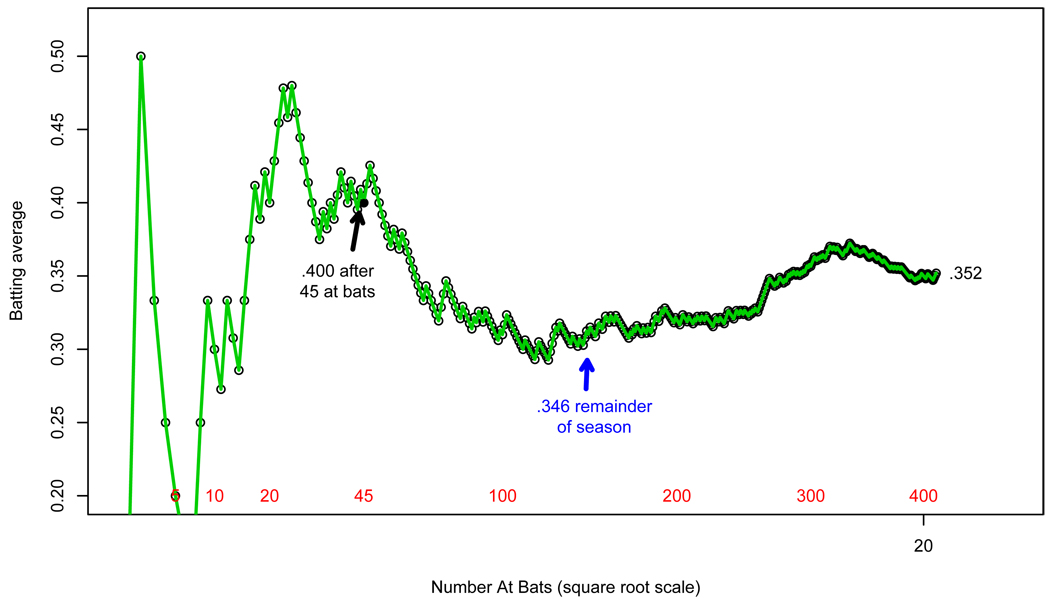
Figure 1 concerns an example of direct statistical evidence, taken from the sports pages of 1970. We are following the star baseball player Roberto Clemente through his 1970 season. His batting average, number of successes (“hits”) over number of tries (“at bats”) fluctuates wildly at first but settles down as the season progresses. After 45 tries he has 18 hits, for a batting average of 18/45 = .400 or “four hundred” in baseball terminology. The remainder of the season is slightly less successful, with 127 hits out of 367 at bats for a batting average of .346 = 127/367, giving Clemente a full season average of .352¹ This is a classic frequentist estimate: direct statistical evidence for Clemente’s 1970 batting ability.

Figure 1.

Roberto Clemente’s batting averages over the 1970 baseball season (partially simulated). After 45 tries he had 18 hits for a batting average of 18/45 = .400; his average in the remainder of the season was 127/367 = .346.

In contentious areas such as drug efficacy, the desire for direct evidence can be overpowering. A clinical trial often has three arms: placebo, single dose of new drug, and double dose. Even if the double dose/placebo comparison yields strongly significant results in favor of the new drug, a not-quite significant result for the single dose/placebo comparison, say p-value .07, will not be enough to earn FDA approval. The single dose by itself must prove its worth.

My own feeling at this point would be that the single dose is very likely to be vindicated in any subsequent testing. The strong result for the double dose adds indirect evidence to the direct, nearly significant, single dose outcome. As the talk’s title suggests, indirect statistical evidence is the focus of interest here. My main point, which will take a while to unfold, is that current scientific trends are producing larger and more complex data sets in which indirect evidence has to be accounted for: and these trends will force some re-thinking of both frequentist and Bayesian practices.

3 Bayesian Inference

I was having coffee with a physicist friend and her husband who, thanks to the miracle of sonograms, knew they were due to have twin boys. Without warning, the mother-to-be asked me what was the probability her twins would be identical rather than fraternal. Stalling for time, I asked if the doctor had given her any further information. “Yes, he said the proportion of identical twins is one-third.” (I checked later with an epidemiology colleague who confirmed this estimate.)

Thomas Bayes, 18th-century non-conformist English minister, would have died in vain if I didn’t use his rule to answer the physicist mom. In this case the prior odds

$$\frac{\text{Pr}\left\{\text{Identical}\right\}}{\text{Pr}\left\{\text{Fraternal}\right\}}=\frac{1/3}{2/3}=\frac{1}{2}$$

favor fraternal. However the likelihood ratio, the current evidence from the sonogram, favors identical,

$$\frac{\text{Pr}\{\text{Twin}\text{Boys}|\text{Identical}\}}{\text{Pr}\{\text{Twin}\text{Boys}|\text{Fraternal}\}}=2,$$

since identical twins are always the same sex while fraternal twins are of differing sexes half the time.

Bayes rule, published posthumously in 1763, is a rule for combining evidence from different sources. In this case it says that the posterior odds of identical to fraternal is obtained by simple multiplication.

$$\begin{array}{cc}\text{Posterior}\text{Odds}\hfill & =(\text{Prior}\text{Odds})\cdot (\text{Likelihood}\text{Ratio})\hfill \\ \hfill & =\frac{1}{2}\cdot 2=1.\hfill \end{array}$$

So my answer to the physicists was “50/50,” equal chances of identical or fraternal. (This sounded like pure guessing to them; I would have gotten a lot more respect with “60/40.”)

Bayes rule is a landmark achievement. It was the first breakthrough in scientific logic since the Greeks and the beginning of statistical inference as a serious mathematical subject. From the point of view of this talk, it also marked the formal introduction of indirect evidence into statistical learning.

Both Clemente and the physicists are learning from experience. Clemente is learning directly from his own experience, in a strict frequentist manner. The physicists are learning from their own experience (the sonogram), but also indirectly from the experience of others: that one-third/two-thirds prior odds is based on perhaps millions of previous twin births, mostly not of the physicists’ “twin boys” situation. Another way to state Bayes rule is as a device for filtering out and using the relevant portions of past experiences.

All statisticians, or almost all of them, enjoy Bayes rule but only a minority make much use of it. Learning only from direct experience is a dominant feature of contemporary applied statistics, connected, as I said, with notions of scientific objectivity. A fundamental Bayesian difficulty is that well-founded prior distributions, like the twins one-thirds/two-thirds, are rare in scientific practice. Much of 20th-century Bayesian theory concerned subjective prior distributions, which are not very convincing in contentious areas such as drug trials.

The holy grail of statistical theory is to use the experience of others without the need for subjective prior distributions: in L.J. Savage’s words, to enjoy the Bayesian omelette without breaking the Bayesian eggs. I am going to argue that this grail has grown holier, and more pressing, in the 21st century. First though I wanted to say something about frequentist use of indirect information.

4 Regression Models

Bayesians have an advantage but not a monopoly on the use of indirect evidence. Regression models provide an officially sanctioned² frequentist mechanism for incorporating the experience of others.

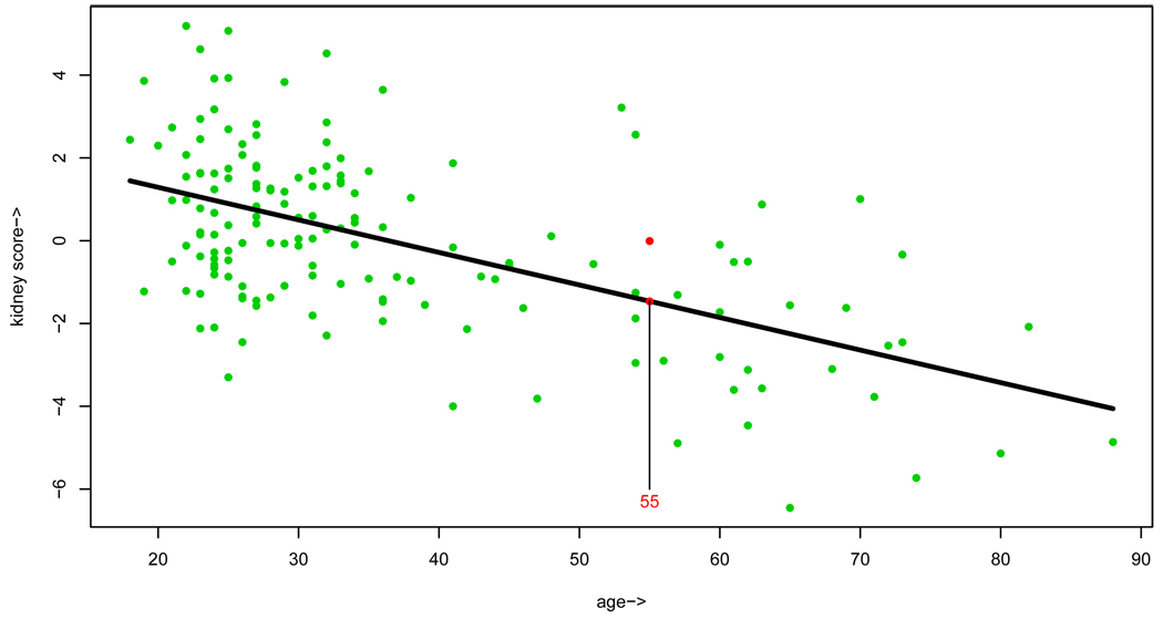
Figure 2 concerns an example from Dr. Brian Myers’ Stanford nephrology laboratory: 157 healthy volunteers have had their kidney function evaluated by a somewhat arduous series of tests. An overall kidney score, higher numbers better, is plotted versus the volunteer’s age, illustrating a decline in function among the older subjects. (Kidney donation was once limited to volunteers less than 60 years old.) The decline is emphasized by the downward slope of the least squares regression line.

Figure 2.

Kidney function plotted versus age for 157 healthy volunteers from the nephrology laboratory of Dr. Brian Myers. The least squares regression line has a strong downward slope. A new donor age 55 has appeared, and we need to predict his kidney score.

A potential new donor, age 55, has appeared but it is not practical to evaluate his kidney function by the arduous testing procedure. How good are his kidneys? As far as direct evidence is concerned, only one of the 157 volunteers was 55, and he had score −.01. Most statisticians would prefer the estimate obtained from the height at age 55 of the least square line, −1.46. In Tukey’s evocative language, we are “borrowing strength” from the 156 volunteers who are not age 55.

Borrowing strength is a clear use of indirect evidence, but invoked differently than through Bayes theorem. Now every individual is adjusted to fit the case of interest; in effect the regression model allows us to adjust each volunteer to age 55. Linear model theory permits a direct frequentist analysis of the entire least squares fitting process, but that shouldn’t conceal the indirect nature of its application to individual cases.

One response of the statistical community to the onslaught of increasingly large and complex data sets has been to extend the reach of regression models: LARS, lasso, boosting, bagging, CART, and projection pursuit being a few of the ambitious new data-mining algorithms. Every self-respecting sports program now has its own simplified data-mining program, producing statements like “Jones has only 3 hits in 16 tries versus Pettitte.” This is direct evidence run amok. Regression models seem to be considered beyond the sporting public’s sophistication, but indirect evidence is everywhere in the sports world, as I want to discuss next.

5 James–Stein Estimation

Early in the 1970 baseball season, Carl Morris collected the batting average data shown in the second column of Table 1. Each of the 18 players had batted 45 times (they were all of those who had done so) with varying degrees of success. Clemente, as shown in Figure 1, had hit successfully 18 of the 45 times, for an observed average of .400 = 18/45. Near the bottom of the table, Thurman Munson, another star player, had only 8 hits; observed average 8/45 = .178. The grand average of the 18 players at that point was .265.

Table 1.

Batting averages for 18 major league players early in the 1970 season (“Observed”) and their averages for the remainder of the season (“Truth”). Also the James–Stein predictions.

Name	Hits/AB	Observed	“Truth”	James–Stein
1. Clemente	18/45	.400	.346	0.294
2. F. Robinson	17/45	.378	.298	0.289
3. F. Howard	16/45	.356	.276	0.285
4. Johnstone	15/45	.333	.222	0.280
⋮	⋮	⋮	⋮	⋮
14. Petrocelli	10/45	.222	.264	0.256
15. E. Rodriguez	10/45	.222	.226	0.256
16. Campaneris	9/45	.200	.286	0.252
17. Munson	8/45	.178	.316	0.247
18. Alvis	7/45	.156	.200	0.242
Grand Average		.265	.265	0.265

Only about one-tenth of the season had elapsed, and Morris considered predicting each player’s subsequent batting average during the remainder of 1970. Since the players bat independently of each other – Clemente’s successes don’t help Munson, nor vice versa – it seems there is no alternative to using the observed averages, at least not without employing more baseball background knowledge.

However, that is not true. The James–Stein estimates in the last column of the table are functions of the observed averages, obtained by shrinking them a certain amount of the way toward the grand average .265, as described next. By the end of the 1970 season, Morris could see the “truth”, the players’ averages over the remainder of the season. If prediction error is measured by total squared discrepancy from the truth, then James–Stein wins handsomely: its total squared prediction error was less than one-third of that for the observed averages. This wasn’t a matter of luck, as we will see.

Suppose each player has a true expectation μ_i and an observed average x_i, following the model

$${\mu }_i~𝒩(M,A)\text{\hspace{1em}and\hspace{1em}}{x}_i|{\mu }_i\sim 𝒩({\mu }_i,{\sigma }_0^2)$$ (1)

for i = 1, 2, …, N = 18. Here M and A are mean and variance hyper-parameters that determine the Bayesian prior distribution; μ_i can be thought of as the “truth” in Table 1, x_i as the observed average, and ${\sigma }_0^2$ as its approximate binomial variance .265·(1–.265)/45. (I won’t worry about the fact that x_i is binomial rather than perfectly normal.)

The posterior expectation of μ_i given x_i, which is the Bayes estimator under squared error loss, is

$${\widehat{\mu }}_i^{(\text{Bayes})}=M+B(x_i-M)\text{\hspace{1em}where}B=\frac{A}{A+{\sigma }_0^2}.$$ (2)

If $A={\sigma }_0^2$ for example, Bayes rule shrinks each observed average x_i half-way toward the prior mean M. Using Bayes rule reduces the total squared error of prediction, compared to using the obvious estimates x_i, by a factor of 1 − B. This is a 50% savings if $A={\sigma }_0^2$, and more if the prior variance A is less than ${\sigma }_0^2$.

Baseball experts might know accurate values for M and A, or M and B, but we are not assuming expert prior knowledge here. The James–Stein estimator can be motivated quite simply: unbiased estimates M̂ and B̂ are obtained from the vector of observations x = (x₁, x₂, …, x_N) (e.g., M̂ = x̄ the grand average) and substituted into formula (2). In Herbert Robbins' apt terminology, James–Stein is an empirical Bayes estimator. It doesn’t perform as well as the actual Bayes estimate (2), but under model (1) the penalty is surprisingly small.

All of this seems interesting enough, but a skeptic might ask where the normal prior distributions ${\mu }_i\stackrel{\text{ind}}{~}𝒩(M,A)$ in (1) are coming from. In fact, James and Stein didn’t use normal priors, or any priors at all, in their derivation. Instead they proved the following frequentist theorem.

Theorem 1 (1956)

If $x_i~𝒩({\mu }_i,{\sigma }_0^2)$ independently for i = 1, 2, …, N, N ≥ 4, then the James–Stein estimator always beats the obvious estimator x_i in terms of expected total squared estimation error.

This is the single most striking result of post-World War II statistical theory. It is sometimes called³ Stein’s paradox for it says that Clemente’s good performance does increase our estimate for Munson (e.g., by increasing M̂ = x̄) and vice versa, even though they succeed or fail independently. In addition to the direct evidence of each player’s batting average, we gain indirect evidence from the other 17 averages.

James–Stein estimation is not an unmitigated blessing. Low total squared error can conceal poor performance on genuinely unusual cases. Baseball fans know from past experience that Clemente was an unusually good hitter, who is learning too much from the experience of others by being included in a cohort of less-talented players. I’ll call this the Clemente problem in what follows.

6 Large-Scale Multiple Inference

All of this is a preface, and one that could have been written 50 years ago, to what I am really interested in talking about here. Large-scale multiple inference, in which thousands of statistical problems are considered at once, has become a fact of life for 21st-century statisticians. There is just too much indirect evidence to ignore in such situations. Coming to grips with our new, more intense, scientific environment is a major enterprise for the statistical community, and one that is already affecting both theory and practice.

Rupert Miller’s book Simultaneous Statistical Inference appeared in 1966, lucidly summarizing the post-war boom in multiple-testing theory. The book is overwhelmingly frequentist, aimed mainly at the control of type I error, and concerned with the simultaneous analysis of between 2 and perhaps 10 testing problems. Microarray technology introduced in the 1990s dramatically raised the ante: number of problems N now easily exceeds 10,000; “SNP chips” have N = 500, 000+, and imaging devices reach higher still.

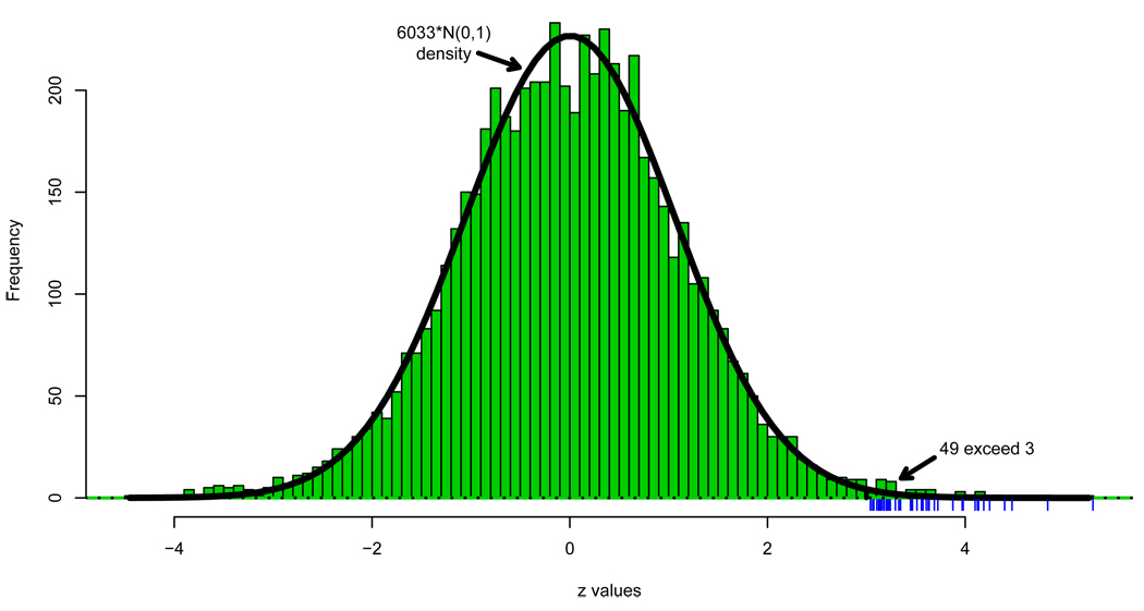
Figure 3 concerns a microarray study in which the researchers were on a fishing expedition to find genes involved in the development of prostate cancer: 102 men, 50 healthy controls and 52 prostate cancer patients, each had expression levels for N = 6033 genes measured on microarrays. The resulting data matrix had N = 6033 rows, one for each gene, and 102 columns, one for each man.

Figure 3.

Histogram of N = 6033 z-values from the prostate cancer study compared with the theoretical null density that would apply if all the genes were uninteresting. Hash marks indicate the 49 z-values exceeding 3.0.

As a first step in looking for “interesting” genes, a two-sample t-statistic t_i comparing cancer patients with controls was computed for each gene i, i = 1, 2,…,N, and then converted to a z-value

$$z_i={\mathbf{\Phi }}^{-1}(F_{100}(t_i))$$ (3)

with Φ and F₁₀₀ the cdfs of a standard normal and t₁₀₀ variate. Under the usual textbook conditions, z_i will have a standard normal distribution in the null (uninteresting) situation where genetic expression levels are identically distributed for controls and patients,

$$H_0:z_i\sim 𝒩(0,1).$$ (4)

A histogram of the N = 6033 z-values appears in Figure 3. It is fit reasonably well by the “theoretical null” curve that would apply if all the genes followed (4), except that there is an excess of tail values, which might indicate some interesting “non-null” genes responding differently in cancer and control subjects.

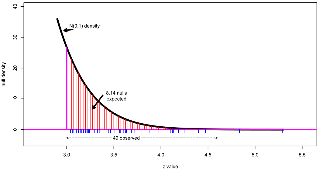
Here I will concentrate on the 49 genes having z_i exceeding 3.0, as indicated by the hash marks. Figure 4 shows a close-up of the right tail, where we notice that 49 is much greater than 8.14, the expected number of z_i’s exceeding 3.0 under full null conditions. The ratio is

$$\widehat{\text{Fdr}}(3.0)=\frac{8.14}{49}=\frac{1}{6}.$$ (5)

where Fdr stands for false discovery rate, in Benjamini and Hochberg’s evocative terminology. Reporting the list of 49 back to the investigators seems like a good bet if it only contains 1/6 duds, but can we believe that value?

Figure 4.

Close-up of right tail of the prostate data z-value histogram; 49 z_i’s exceed 3.0, compared to an expected number 8.14 if all genes were null (4).

Benjamini and Hochberg’s 1995 paper answered the question with what I consider the second most striking theorem of post-war statistics. For any given cutoff point c let N(c) be the number of z_i's observed to exceed c, E₀(c) the expected number exceeding c if all genes are null (4), and

$$\widehat{\mathrm{\text{Fdr}}}(c)=E_0(c)/N(c).$$ (6)

(In (5), c = 3.0, N(c) = 49, and E₀(c) = 8.14.) Choose an Fdr control value q between 0 and 1 and let c_q be the smallest value of c such that $\widehat{\text{Fdr}}(c)\le q$.

Theorem 2

If the N z-values are independent of each other, then the rule that rejects the null hypothesis (4)for all cases having z_i ≥ c_q will make the expected proportion of false discoveries no greater than q.

In the prostate data example, choosing q = 1/6 gives c_q = 3.0 and yields a list of 49 presumably interesting genes. Assuming independence⁴, the theorem says that the expected proportion of actual null cases on the list is no greater than 1/6. That is a frequentist expectation, Benjamini and Hochberg like James and Stein having worked frequentistically, but once again there is an instructive Bayesian interpretation.

A very simple Bayes model for simultaneous hypothesis testing, the two-groups model, assumes that each gene has prior probability p₀ or p₁ = 1 – p₀ of being null or non-null, with corresponding z-value density f₀(z) or f₁(z):

$$\text{Prior}\text{Probability}\{\begin{array}{c}{p}_0\hfill \\ p_1\hfill \end{array}{z}_i\sim \{\begin{array}{c}{f}_0(z)\hfill \\ f_1(z)\hfill \end{array}.$$ (7)

Let F₀(z) and F₁(z) be the right-sided cdfs (survival functions) corresponding to f₀ and f₁, and F(z) their mixture,

$$F(z)=p_0{F}_0(z)+p_1{F}_1(z).$$ (8)

Applying Bayes theorem shows that the true false discovery rate is

$$\text{Fdr}(c)\equiv \text{Pr}\{\text{gene}i\text{null}|z_i\ge c\}=p_0{F}_0(c)/F(c).$$ (9)

(Left-sided cdfs perform just as well, but it is convenient to work on the right here.)

Of course we can’t apply the Bayesian result (9) unless we know p₀, f₀, and f₁ in (7). Once again though, a simple empirical Bayes estimate is available. Under the theoretical null (4), F₀(z) = 1 − Φ(z), the standard normal right-sided cdf; p₀ will usually be close to 1 in fishing expedition situations and has little effect on Fdr(c). (Benjamini and Hochberg set p₀ = 1. It can be estimated from the data, and I will take it as known here.) That leaves the mixture cdf F(z) as the only unknown. But by definition, all N z_i values follow F(z), so we can estimate it by the empirical cdf F̂(z) = #{z_i ≥ z}/N, leading to the empirical Bayes estimate of (9),

$$\widehat{\text{Fdr}}(c)=p_0{F}_0(c)/\widehat{F}(c).$$ (10)

The two definitions of $\widehat{\text{Fdr}}(c)$, (6) and (10), are the same since E₀(c) = N_p0F₀(c) and F̂(c) = N(c)/N. This means we can restate Benjamini and Hochberg’s theorem in empirical Bayes terms: the list of cases reported by BH(q), the Benjamini–Hochberg-level q rule, is essentially those cases having estimated posterior probability of being null no greater than q.

The Benjamini–Hochberg algorithm clearly involves indirect evidence. In this case, each z-value is learning from the other N − 1 values: if, say, only 10 instead of 49 z-values had exceeded 3.0, then $\widehat{\text{Fdr}}(c)$ would equal .81 (i.e., “very likely null”) so a gene with z_i ≥ 3.0 would now not be reported as non-null.

I have been pleasantly surprised at how quickly false discovery rate control was accepted by statisticians and our clients. It is fundamentally different from type I error control, the standard for nearly a century, in its Bayesian aspect, its use of indirect evidence, and in the fact that it provides an explicit estimate of nullness $\widehat{\text{Fdr}}(z)$ rather than just a yes/no decision.⁵

7 The Proper Use of Indirect Evidence

The false discovery rate story is a promising sign of our professions’ ability to embrace new methods for new problems. However, in moving beyond the confines of classical statistics we are also moving outside the wall of protection that a century of theory and experience has erected against inferential error.

Within its proper venue, it is hard to go very wrong with a frequentist analysis of direct evidence. I find it quite easy to go wrong in large-scale data analyses. This section and the next offer a couple of examples of the pitfalls yawning in the use of indirect evidence. None of this is meant to be discouraging: difficulties are what researchers thrive on, and I fully expect statisticians to successfully navigate these new waters.

The results of another microarry experiment, this time concerning leukemia, are summarized in Figure 5. High density oligonucleotide microarrays provided expression levels on N = 7128 genes for 72 patients, 45 with ALL (acute lymphoblastic leukemia) and 27 with AML (acute myeloid leukemia), the latter having worse prognosis. Two-sample t-statistics provided z-values z_i for each gene, as with the prostate study.

Figure 5.

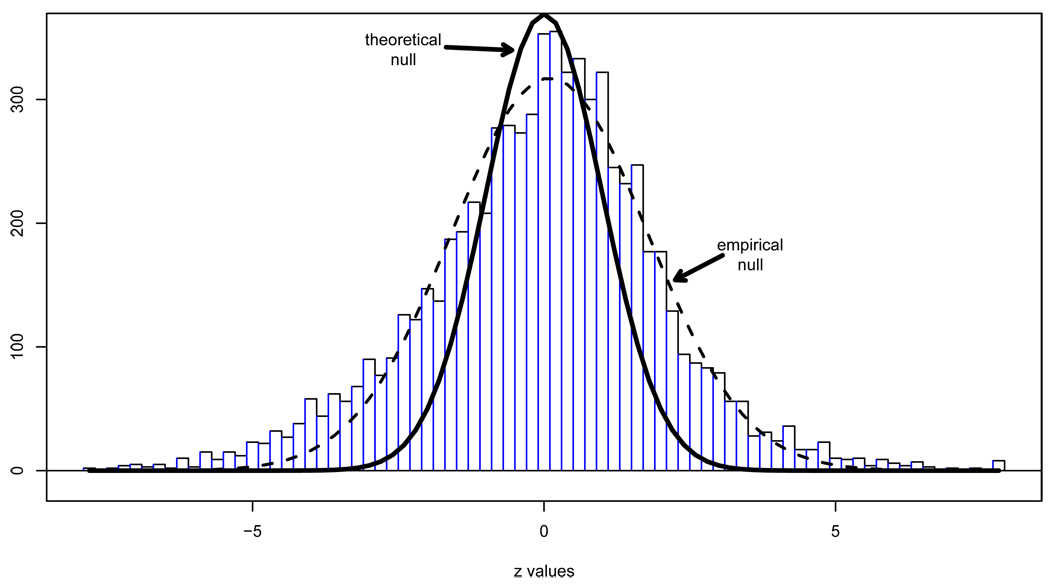
Histogram of z-values for N = 7128 genes in a microarray study comparing two types of leukemia. The N(0, 1) theoretical null is much narrower than the histogram center; a normal fit to the central histogram height gives empirical null N(.09, 1.68²). Both curves have been scaled by their respective estimates of p₀ in (7).

Figure 5 shows that this time the center of the z-value histogram does not approximate a N(0, 1) density. Instead, it is much too wide: a maximum likelihood fit to central histogram heights gave estimated proportion p₀ = .93 of null genes in the two-groups model (7), and an empirical null density estimate

$$f_0(z)\sim 𝒩(.09,{1.68}^2),$$ (11)

more than half again as wide as the N(0, 1) theoretical null (4). The dashed curve shows (11) nicely following the histogram height near the center while the estimated proportion of non-null genes p₁ = 1 − p₀ = .07 appear as heavy tails, noticeably on the left.

At this point one could maintain faith in the theoretical null but at the expense of concluding that about 2500 (35%) of the genes are involved in AML/ALL differences. On the other hand, there are plenty of reasons to doubt the theoretical null. In particular, the leukemia data comes from an observational study, not a randomized experiment, so that unobserved covariates (age, sex, health status, race, etc.) could easily add a component of variance to both the null and non-null z-values.

The crucial question here has to do with the numerator E₀(c) in $\widehat{\mathrm{\text{Fdr}}}(c)=E_0(c)/N(c)$, the expected number of null cases exceeding c. The theoretical N(0, 1) null predicts many fewer of these than does the empirical null (11). The fact that we might estimate the appropriate null distribution from evidence at hand — bordering on heresy from the point of view of classical testing theory — shows the opportunities inherent in large-scale studies, as well as the novel inferential questions surrounding the use of indirect evidence.

8 Relevance

Large-scale testing algorithms are usually carried out under the tacit assumption that all available cases should be analyzed together: for instance, employing a single false discovery analysis for all the genes in a given microarray experiment. This can be a dangerous assumption, as the example illustrated in Figure 6 will show.

Figure 6.

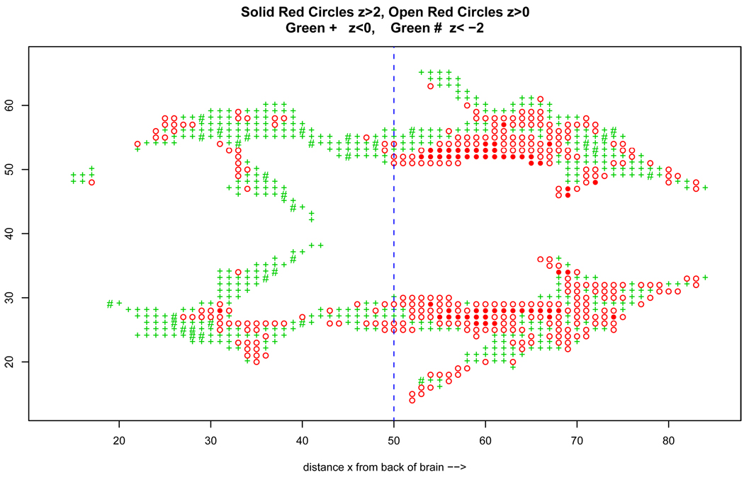
DTI study z-values comparing 6 dyslexic children with 6 normal controls, at N = 15443 voxels; shown is horizontal section of 848 voxels; x indicates distance from back of brain (left) to front (right). The vertical line at x = 50 divides the brain into back and front halves.

Twelve children, six dyslexics and six normal controls, received DTI (diffusion tensor imaging) scans, measuring fluid diffusion at N = 15,443 locations (voxels) in the brain. A z-value z_i was computed at each voxel such that the theoretical null hypothesis z_i ~ N(0, 1) should apply to locations where there is no dyslexic/normal distributional difference. The goal of course was to pinpoint areas of genuine difference.

Figure 6 indicates the z-values in a horizontal slice of the brain about half-way from bottom to top. Open circles, colored red, indicate z_i ≥ 0, solid red circles z_i ≥ 2; green + symbols indicate z_i < 0, with green # for z_i < −2. The x-axis measures distance from the back of the brain to the front, left to right.

Spatial correlation among the z_i’s is evident: red circles are near red circles and green +’s near other green +'s. The Benjamini–Hochberg Fdr control algorithm tends to perform as claimed as an hypothesis-testing device, even under substantial correlation. However, there is an empirical Bayes price to pay: correlation makes $\widehat{\text{Fdr}}(c)$ (10) less dependable as an estimate of the true Bayes probability (9). Just how much less is a matter of current study.

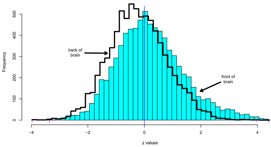
There is something else to worry about in Figure 6: the front half of the brain, x ≥ 50, seems to be redder (i.e., with more positive z-values) than the back half. This is confirmed by the superimposed histograms for the two halves, about 7,700 voxels each, seen in Figure 7. Separate Fdr tests at control level q = .10 yield 281 “significant” voxels for the front-half data, all those with z_i ≥ 2.69, and none at all for the back half. But if we analyze all 15443 voxels at once, the Fdr test yields only 198 significant voxels, those having z_i ≥ 3.02. Which analysis is correct?

Figure 7.

Separate histograms for z_i’s from the front and back halves of the brain, DTI study. The heavy right tail of the front-half data yields 281 significant voxels in an Fdr test, control level q = .10.

This is the kind of question my warning about difficult new inference problems was aimed at. Notice that the two histograms differ near their centers as well as in the tails. The Fdr analyses employed thoretical N(0, 1) null distributions. Using empirical nulls as with the leukemia data gives quite different null distributions, raising further questions about proper comparisons.

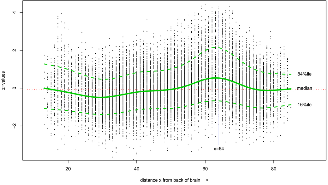
The front/back division of the brain was arbitrary and not founded on any scientific criteria. Figure 8 shows all 15,443 z_i’s plotted against x_i, the voxel’s distance from the back. We see waves in the z-values, at the lower percentiles as well as at the top, cresting near x = 64. Disturbingly, most of the 281 significant voxels for the front-half analysis came from this crest.

Figure 8.

z-values for the 15,443 voxels plotted versus their distance from the back of the brain. A disturbing wave pattern is evident, cresting near x = 64. Most of the 281 significant voxels in Figure 7 come from this crest.

Maybe I should be doing local Fdr tests of some sort, or perhaps making regression adjustments (e.g., subtracting off the running median) before applying an Fdr procedure. We have returned to a version of the Clemente problem: which are the relevant voxels for deciding whether or not any given voxel is responding differently in dyslexics and controls? In other words, where is the relevant indirect information?

9 The Normal Hierarchical Model

My final example of indirect evidence and empirical Bayes inference concerns the normal hierarchical model. This is a simple but important Bayesian model where μ, a parameter of interest, comes from some prior density g(·) and we get to observe a normal variate z centered at μ,

$$\mu \sim g(\cdot )\text{\hspace{1em}and\hspace{1em}}z|\mu \sim 𝒩(\mu ,1).$$ (12)

Both the James–Stein and Benjamini–Hochberg estimators can be motivated from (12),

$$\text{JS}:g=𝒩(M,A)\text{\hspace{1em}and\hspace{1em}BH}:g=p_0{\delta }_0+p_1{g}_1.$$ (13)

In the latter, δ₀ is a delta function at 0 while g₁ is an arbitrary density giving f₁ in (7) by convolution, f₁ = g₁ * φ where φ is the standard normal density.

In the BH setting, we might call μ_i (the value of μ for the ith case) the effect size. For prediction purposes, we want to identify cases not only with μ_i ≠ 0 but with large effect size. A very useful property of the normal hierarchical model (12) allows us to calculate the Bayes estimate of effect size directly from the convolution density f = g * φ without having to calculate g,

$$f(z)={\displaystyle {\int }_{-\mathrm{\infty }}^{\mathrm{\infty }}\phi (z-\mu )g(\mu )d\mu .}$$ (14)

Lemma 1

Under the normal hierarchical model (12),

$$E\{\mu |z\}=z+f\prime (z)/f(z)$$ (15)

where f′(z) = df(z)/dz.

The marginal density of z in model (12) is f(z). So if we observe z = (z₁, z₂, …,z_N) from repeated realizations of (μ_i, z_i), we can fit a smooth density estimate f̂(z) to the z_i’s and use the lemma to approximate E{μ_i|z_i},

$$\mathit{z}\to \widehat{f}(z)\to \widehat{E}\{{\mu }_i|z_i\}=z_i+\widehat{f}\prime (z_i)/f(z_i).$$ (16)

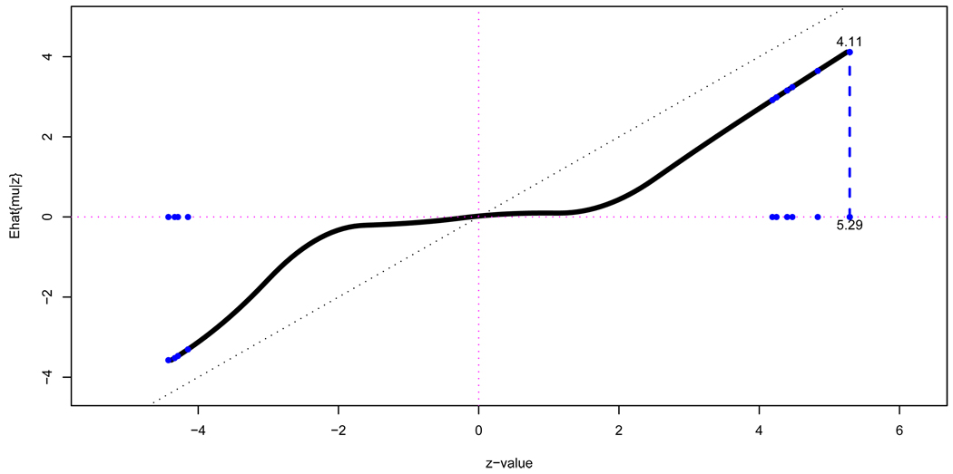
This has been done in Figure 9 for the prostate data of Figure 3, with f̂(z) a natural spline, fit with 7 degrees of freedom to the heights of Figure 3’s histogram bars (all of them, not just the central ones we used to estimate empirical nulls).

Figure 9.

Empirical Bayes effect size estimate Ê{μ|z} (16), prostate data of Figure 3. Dots indicate the top 10 genes, those with the greatest values of |z_i| The top gene, i = 610, has z_i = 5.29 and estimated effect size 4.11.

The effect size estimates μ̂_i = Ê{μ_i|z_i} are nearly zero for |z_i| less than 2 but increase linearly outside of this interval. Gene 610 has the largest z-value, z₆₁₀ = 5.29, with estimated effect size μ̂₆₁₀ = 4.11. Table 2 shows the top 10 genes in order of |z_i|, and their corresponding effect sizes μ̂_i. The μ̂_i values are shrunk toward the origin, but in a manner appropriate to the BH prior in (13), not JS.

Table 2.

Top 10 genes, those with largest values of |z_i|, in the prostate study and their corresponding effect size estimates μ̂_i.

	gene	z-value	μ̂i = Ê {μi|zi}
1	610	5.29	4.11
2	1720	4.83	3.65
3	332	4.47	3.24
4	364	−4.42	−3.57
5	914	4.40	3.16
6	3940	−4.33	−3.52
7	4546	−4.29	−3.47
8	1068	4.25	2.99
9	579	4.19	2.92
10	4331	−4.14	−3.30

The necessity for shrinkage reflects selection bias: the top 10 genes were winners in a competition with 6023 others; in addition to being “good” in the sense of having genuinely large effect sizes, they’ve probably been “lucky” in that their random measurement errors were directed away from zero. Regression to the mean is another name for the shrinkage effect.

A wonderful fact is that Bayes estimates are immune to selection bias! If μ̂₆₁₀ = 4.11 was the actual Bayes estimate E{μ₆₁₀|z} then it would not matter that we became interested in Gene 610 only after examining all 6033 z-values: 4.11 would still be our estimate. This may seem surprising, but it follows immediately from Bayes theorem, a close cousin to results such as “Bayes inference in a clinical trial is not affected by intermediate looks at the data.”

Any assumption of a Bayes prior is a powerful statement of indirect evidence. In our example it amounts to saying “We have an infinite number N of relevant prior observations (μ, z) with z = 5.29, and for those the average value of μ is 4.11.” The N = ∞ prior observations outweigh any selection effects in the comparatively puny current sample, which is another way of stating the wonderful fact.

Of course, we usually don’t have an infinite amount of relevant past experience. Our empirical Bayes estimate μ̂₆₁₀ = 4.11 is based on just the N = 6033 observed z_i values. One might ask how immune are empirical Bayes estimates to selection bias? This is the kind of important indirect- evidence question that I’m hoping statisticians will soon be able to answer.

10 Learning From the Experience of Others

As I said earlier, current statistical practice is dominated by frequentist methodology based on direct evidence. I don’t believe this kind of single-problem N = 1 thinking, even supplemented by aggressive regression technology, will carry the day in an era of enormous data sets and large-scale inferences. The proper use of indirect evidence — learning from the experience of others — is a pressing challenge for both theoretical and applied statisticians. Perhaps I should just say that frequentists need to become better Bayesians.

This doesn’t let Bayesians off the hook. A “theory of everything” can be a dangerous weapon in the messy world of statistical applications. The tacit assumption of having N = ∞ relevant past cases available for any observed value of the data can lead to a certain reckless optimism in one’s conclusions. Frequentism is a leaky philosophy but a good set of work rules. Its fundamentally conservative attitude encourages a careful examination of what can go wrong as well as right with statistical procedures and, as I’ve tried to say, there’s no shortage of wrong steps possible in our new massive-data environment.

Fisherian procedures, which I haven’t talked about today, often provide a pleasant compromise between Bayesian and frequentist methodology. Maximum likelihood estimation in particular can be interpreted from both viewpoints, as a preferred way of combining evidence from different sources. Fisher’s theory was developed in a small-sample direct-evidence framework, however, and doesn’t answer the questions raised here. Mainly it makes me hope for a new generation of Fishers, Neymans, Hotellings, etc., to deal with 21st-century problems.

Empirical Bayes methods seem to me to be the most promising candates for a combined Bayesian/frequentist attack on large-scale data analysis problems, but they have been “promising” for 50-plus years now, and have yet to form into a coherent theory. Most pressingly, both frequentists and Bayesians enjoy convincing information theories saying how well one can do in any given situation, while empirical Bayesians still operate on an ad hoc basis.

This is an exciting time to be a statistican: we have a new class of difficult but not impossible problems to wrestle with, which is the most any intellectual discipline can hope for. The wrestling process is already well underway, as witnessed in our journals and conferences. Like most talks that have “future” in the title, this one will probably seem quaint and limited not very long from now, but perhaps the discussants will have more to say about that.

References

- Benjamini Y, Hochberg Y. Controlling the false discovery rate: a practical and powerful approach to multiple testing. J. Roy. Statist. Soc. Ser. B. 1995;57:289–300. [the original Fdr paper] [Google Scholar]
- Benjamini Y, Yekutieli D. False discovery rate-adjusted multiple confidence intervals for selected parameters. J. Amer. Statist. Assoc. 2005;100:71–93. [a frequentist confidence interval approach for effect size estimation] [Google Scholar]
- Brown LD. Admissible estimators, recurrent diffusions, and insoluble boundary value problems. Ann. Math. Statist. 1971;42:855–903. [early use of the normal hierarchical model and its lemma] [Google Scholar]
- Efron B. R.A. Fisher in the 21st century (invited paper presented at the 1996 R.A. Fisher Lecture) Statist. Sci. 1998;13:95–122. [Fisherian inference as a compromise between Bayesian and frequentist methods] [Google Scholar]
- Efron B. Robbins, empirical Bayes and microarrays. Ann. Statist. 2003;31:366–378. [a brief review of Herbert Robbins’ pathbreaking empirical Bayes work] [Google Scholar]
- Efron B. Large-scale simultaneous hypothesis testing: The choice of a null hypothesis. J. Amer. Statist. Assoc. 2004;99:96–104. [the empirical null] [Google Scholar]
- Efron B. Microarrays, empirical Bayes and the two-groups model. Statist. Sci. 2008a;23:1–22. [a long review, with discussion, of false discovery rates] [Google Scholar]
- Efron B. Simultaneous inference: When should hypothesis testing problems be combined? Ann. Appl. Statist. 2008b;2:197–223. [concerns “relevance” and the DTI example] [Google Scholar]
- Efron B. Empirical bayes estimates for large-scale prediction problems. J. Amer. Statist. Assoc. 2009 doi: 10.1198/jasa.2009.tm08523. to appear [effect size estimation] [DOI] [PMC free article] [PubMed] [Google Scholar]
- Efron B, Morris C. Stein’s paradox in statistics. Scientific American. 1977;236:119–127. [Google Scholar]
- Golub TR, Slonim DK, Tamayo P, Huard C, Gaasenbeek M, Mesirov JP, Coller H, Loh ML, Downing JR, Caligiuri MA, Bloomfield CD, Lander ES. Molecular Classification of Cancer: Class Discovery and Class Prediction by Gene Expression Monitoring. Science. 1999;286:531–537. doi: 10.1126/science.286.5439.531. [the leukemia data] [DOI] [PubMed] [Google Scholar]
- Hastie T, Tibshirani R, Friedman J. Springer Series in Statistics. 2nd ed. New York: Springer-Verlag; 2008. The Elements of Statistical Learning. [a wide-ranging review of modern regression techniques] [Google Scholar]
- Lemley KV, Lafayette RA, Derby G, Blouch KL, Anderson L, Efron B, Myers BD. Prediction of early progression in recently diagnosed IgA nephropathy. Nephrol. Dialysis Transplant. 2008;23:213–222. doi: 10.1093/ndt/gfm560. [the kidney data] [DOI] [PubMed] [Google Scholar]
- Miller RG., Jr . Springer Series in Statistics. 2nd ed. New York: Springer-Verlag; 1981. Simultaneous Statistical Inference. [a classic review of post-war multiple inference] [Google Scholar]
- Schwartzman A, Dougherty R, Taylor J. Cross-subject comparison of principal diffusion direction maps. Magn. Reson. Med. 2005;53:1423–1431. doi: 10.1002/mrm.20503. [DTI data analysis] [DOI] [PMC free article] [PubMed] [Google Scholar]
- Senn S. A note concerning a selection “paradox” of Dawid’s. Amer. Statist. 2008;62:206–210. [nice discussion of Bayesian “immunity”, referring to Phil Dawid’s original work] [Google Scholar]
- Singh D, Febbo PG, Ross K, Jackson DG, Manola J, Ladd C, Tamayo P, Renshaw AA, D’Amico AV, Richie JP, Lander ES, Loda M, Kantoff PW, Golub TR, Sellers WR. Gene expression correlates of clinical prostate cancer behavior. Cancer Cell. 2002;1:203–209. doi: 10.1016/s1535-6108(02)00030-2. [prostate cancer study] [DOI] [PubMed] [Google Scholar]
- Stein CM. Inadmissibility of the usual estimator for the mean of a multivariate normal distribution; In Proceedings of the Third Berkeley Symposium on Mathematical Statistics and Probability 1954–1955; Berkeley and Los Angeles: University of California Press; 1956. pp. 197–206. [original exposition of “Stein’s paradox”] [Google Scholar]