Conformational Statistics of Semi-Flexible Macromolecular Chains with Internal Joints

Abstract

Fluctuations in the bending angles at internal irregularities of DNA and RNA (such as symmetric loops, bulges, and nicks/gaps) have been observed from various experiments. However, little effort has been made to computationally predict and explain the statistical behavior of semi-flexible chains with internal defects. In this paper, we describe the general structure of these macromolecular chains as inextensible elastic chains with one or more internal joints which have limited ranges of rotation, and propose a method to compute the probability density functions of the end-to-end pose of these macromolecular chains. Our method takes advantage of the operational properties of the non-commutative Fourier transform for the group of rigid-body motions in three-dimensional space, SE(3). Two representative types of joints, the hinge for planar rotation and the ball joint for spatial rotation, are discussed in detail. The proposed method applies to various stiffness models of semi-flexible chain-like macromolecules. Examples are calculated using the Kratky-Porod model with specified stiffness, angular fluctuation, and joint locations. Entropic effects associated with internal angular fluctuations of semi-flexible macromolecular chains with internal joints can be computed using this formulation. Our method also provides a potential tool to detect the existence of internal irregularities.

1. Introduction

The internal bending and flexibility of DNA has attracted considerable attention, because of its important role in packaging, recombination and transcription.

First discovered in the early 1980’s ¹, intrinsically bent DNAs have been observed and studied experimentally ^2–8. Local structures, which are more complex than rigid bends, have also been observed from various experiments. In particular, errors during replication and recombination of double-stranded DNA may result in mismatched basepairs or the insertion/deletion of nucleotides. This results in internal structures such as symmetric loops, bulges, and gaps/nicks. These structures usually have different flexibility than regular double helical DNA, and may result in bends. Usually, these bends are not rigid, but exhibit certain ranges of fluctuation. Based on gel electrophoresis experiments, Guo and Tullius showed that a single-nucleoside gap in a DNA duplex leads to an anisotropic, directional bend in the DNA helix axis ⁹. Moreover, a gap is a site of anisotropic flexibility rather than a static, fixed bend. The bending angle caused by a single gap was estimated at around 12°. Roll et al. reported a fluctuating bending angle centered around 17° at the nick site of DNA based on nuclear magnetic resonance (NMR) experiments and molecular dynamics (MD) simulations ¹⁰. Kahn et al. studied the bending and flexibility induced by symmetric internal loops by gel electrophoresis experiments and cyclization kinetics analysis, and found that the internal loop induced high local isotropic flexibility ¹¹. They reported a root-mean-square (RMS) bending angle of 43°(±5°) for 3-basepair loops, which reflects a fairly wide range of angular distribution. Moreover, the bending angle at a loop is essentially independent of the loop size. Zacharias and Hagerman quantified the bending angles caused by symmetric internal loops in RNA, and reported an RMS angular fluctuation of 16°(±5°) for each basepair in the absence of Mg²⁺, and 13°(±4°) in the presence of Mg^{2+ 12}. As for bulge-induced bending, fluorescence resonance energy transfer (FRET) measurements indicated a bending of 50°–70° for an A3 DNA bulge, and 85°–105° for an A5 DNA bulge ¹³. An NMR study also showed a bending angle of 90°(±14°) for an RNA bulge with five unpaired bases AAUAA ¹⁴, and 73°(±11°) for the A5 RNA bulge ¹⁵. Furthermore, from the results of transient electric birefringence (TEB) measurements, Zacharias and Hagerman gave an estimation of a 10°–20° increment of bending angle induced per extra base ¹⁶. They also stated that a given bulge-induced bend could be regarded as a relatively narrow distribution of angles with a non-zero mean angle. Other works have shown strong agreement with the above results regarding bulge-induced bending ^17–20.

Although much experimental attention has been given to the bending fluctuations caused by internal structures, so far no previous work has been published on how to computationally predict and explain the statistical behavior of macromolecular chains with those internal structures.

In contrast, many models have been put forth to describe the behavior of intrinsically straight semi-flexible macromolecular chains and to explain experimental data. Widely-used models include the freely-jointed chain model ²¹, the Kratky-Porod wormlike chain model ^22–24, Yamakawa helical wormlike chain model ²⁵ and the Marko-Siggia double-helix chain model (describing the double-helix structure of DNA) ^{26, 27}. In our previous work, we proposed a general formulation for inextensible semi-flexible macromolecular chains, which includes several above-mentioned polymer models as subcases ²⁸.

Meanwhile, various computational methods have been developed to estimate the conformational statistics of intrinsically straight macromolecular chains. Common techniques include Monte Carlo, matrix-generator, direct enumeration and path integration ^29–37. For some basic polymer models, closed-form formulas have been derived for the probability distributions of loop length ³⁸, segmental orientations ³⁹, trajectories of a segment ⁴⁰, radius of gyration ⁴¹, end-to-end position and distance ^42–49, and moments ^{46, 49, 50}. In our previous work, we showed that the probability density function (PDF) of the end-to-end pose for the most general model of the inextensible semi-flexible macromolecular chain can be obtained by either solving a diffusion equation or convolving PDFs for short segments of the chain ^{28, 51–53}.

Recently some effort has been given to describing macromolecular chains with internal rigid bends. Models have been proposed to describe the relationship between bending stiffness and DNA sequence ^54–56. Matrix-generator and Monte Carlo methods were the first tools used to study the influence of thermal fluctuation on the size and shape of bent DNA ⁵⁷. While classical semi-flexible polymer theories are in general inadequate to describe the conformational statistics of these systems, Rivetti et al. made an effort to extend the applicability of the KP wormlike chain model to bent DNA, and derived closed-form expressions for the mean square end-to-end distance ⁵⁸. In our previous work, we proposed a general method to compute the full probability distribution of the end-to-end pose for the bent macromolecular chain with arbitrary stiffness and chirality parameters ⁵⁹. Ignoring the interactions between distal segments of the same macromolecular chain, our method applies to semi-flexible inextensible chiral elastic macromolecular chains with internal rigid bends and twists.

In spite of all these efforts, there is still a lack of effective tools to estimate the conformational statistics of semi-flexible chains with a finite number of points of increased flexibility. In this paper, we propose a method capable of computing the PDF of the end-to-end pose for semi-flexible macromolecular chains with internal flexible structures, such as loops, bulges and nicks/gaps, ignoring the interactions between distal segments of the same macromolecular chain. In our work, the internal structures involving a small number of basepairs are treated as joints with limited ranges of rotation. Our method is based on our general statistical model of intrinsically straight inextensible semi-flexible macromolecular chains ²⁸, and uses the concept of the Fourier transform for the group of rigid-body motion in three-dimensional space, SE(3).

In Section 2, we briefly review our general statistical model of intrinsically straight inextensible semi-flexible macromolecular chains, and relevant mathematical background on the Fourier transform for SE(3). In Section 3, we present the idea of reducing the internal flexible structures into joints with limited ranges of motion, introduce a general method for computing the PDF of the end-to-end pose for a jointed macromolecular chain, and derive the formulas for two representative types of joints — the hinge and the ball joint. In section 4, we discuss the extreme case — the completely rigid chain with internal joints, and derive the closed form solution for the PDF of the end-to-end distance. In section 5, we demonstrate with examples how to implement our method to compute the desired PDFs, and discuss the computational results.

2. Review of the general inextensible semi-flexible macromolecular chain model

The method presented in this paper is built on a general model of the intrinsically straight inextensible semi-flexible macromolecular chain which was derived in our previous work ²⁸. We briefly review it in this section.

Given a macromolecular chain, one can define a local frame of reference attached to any point on the backbone of the macromolecular chain such that the Z axis of this frame points along the tangent of the backbone (Fig. 1). The frame of reference at the proximal end of the chain is defined by (R(0),a(0))=(I,0), and the pose of the frame of reference at arclength s with respect to the frame of reference at the proximal end is defined by (R(s),a(s)). Here R(s) is a 3×3 rotation matrix defining the relative orientation at arclength s, a(s) is a 3×1 translation vector defining the relative position, I denotes the 3×3 identity matrix, and L denotes the total arclength of the chain.

Figure 1.

Frames of reference attached to a semi-flexible macromolecular chain. (X_pY_pZ_p) represents the frame of reference at the proximal end, (X_sY_sZ_s) represents the frame of reference at arclength s, and (X_dY_dZ_d) represents the frame of reference at the distal end. In the plot, X axes are not displayed but can be derived from Y and Z axes following the right-hand rule.

Under the assumption that the semi-flexible macromolecular chain is inextensible, and the variation of the conformation of the chain is influenced by Gaussian white noise (i.e. Brownian motion forcing), the PDF of the pose of the frame of reference at arclength s with respect to the frame of reference at the proximal end of the chain can be formulated as the path integral on the group of rotations in three-dimensional space, SO(3) ²⁸

$$f(\mathbf{a},\mathbf{R},s)={\int }_{\mathbf{R}(0)}^{\mathbf{R}(s)}\delta (\mathbf{a}(s)-{\int }_0^s\mathbf{R}(\epsilon ){\mathbf{e}}_{3}d\epsilon )e^{-{\int }_0^{s}U(t)dt}D[\mathbf{R}(s)],$$ (1)

where e₃=[0,0,1]′, and δ(.) is the Dirac delta function. Here U(s) is the elastic energy per unit length measured in units of k_BT, where k_B denotes the Boltzmann constant, and T denotes the temperature. It has the form

$$U(s)=\frac{1}{2}\mathbf{\omega }{(s)}^T\mathbf{B}\mathbf{\omega }(s)-{\mathbf{b}}^T\mathbf{\omega }(s)+c,$$ (2)

where ω(s) is called the spatial angular velocity at arclength s (which replaces time in the current context), B is a 3×3 positive semi-definite symmetric matrix called the stiffness matrix, b is a 3×1 vector describing the chirality, and c is a constant. Many elastic models fit into this general formulation, including the Kratky-Porod model, Yamakawa model and the Marko-Siggia model ²⁸. After some mathematical manipulation, one can obtain from (1) the following partial differential equation on SE(3) which describes the PDF of the pose of the frame of reference at arclength s with respect to the frame of reference at the proximal end of the chain ²⁸

$$\frac{\partial f(\mathbf{a},\mathbf{R},s)}{\partial s}=(\frac{1}{2}\sum _{k,l=1}^3{D}_{lk}{\stackrel{\sim }{X}}_l^R{\stackrel{\sim }{X}}_k^R+\sum _{l=1}^3{d}_l{\stackrel{\sim }{X}}_l^R-{\stackrel{\sim }{X}}_6^R)f(\mathbf{a},\mathbf{R},s),$$ (3)

with the initial condition f(a,R,0)= δ(a)δ(R). In Equation 3, D=B⁻¹, d=−B⁻¹b, and ${\stackrel{\sim }{X}}_i^R$ are the differential operators defined for SE(3) (1≤i≤6).

In our previous works ^{28, 51}, a methodology for solving equations such as (3) was developed using the technique of the Fourier transform for SE(3). The matrix elements of this transform are ^{51, 61}

$${\widehat{f}}_{l^{\prime },m^{\prime };l,m}^r(p,s)={\int }_{SE(3)}f(\mathbf{a},\mathbf{R},s)\overline{U_{l,m;l^{\prime },m^{\prime }}^r(\mathbf{a},\mathbf{R};p)}d\mathbf{R}d\mathbf{a},$$ (4)

where for each r ∈ Z and p ∈ ℜ⁺, U^r(a,R;p) is the irreducible unitary representation matrix of SE(3), p is the frequency factor introduced by the transform, and dRda is the invariant integration measure for SE(3). Applying the Fourier transform for SE(3) on both sides of (3), one can obtain a system of linear ordinary differential equations in the form of

$$\frac{d{\widehat{\mathbf{f}}}^r(p,s)}{ds}={\mathbf{B}}^r(p){\widehat{\mathbf{f}}}^r(p,s),$$ (5)

where B^r is a matrix function that is independent of s under the assumption that the stiffness and chirality of the intrinsically straight macromolecular chain are constant along the whole chain. Solving (5), one obtains

$${\widehat{\mathbf{f}}}^r(p,s)=e^{s{\mathbf{B}}^r(p)}.$$ (6)

Then, the desired PDF can be obtained by the inverse transform ^{51, 61}

$$f(\mathbf{a},\mathbf{R},s)=\frac{1}{2{\pi }^2}\sum _{r=-\infty }^{\infty }\sum _{l^{\prime }=\mid r\mid }^{\infty }\sum _{l=\mid r\mid }^{\infty }\sum _{m^{\prime }=-l^{\prime }}^{l^{\prime }}\sum _{m=-l}^l{\int }_0^{\infty }{\widehat{f}}_{l,m;l^{\prime },m^{\prime }}^r(p,s)U_{l^{\prime },m^{\prime };l,m}^r(\mathbf{a},\mathbf{R};p)p^{2}dp.$$ (7)

3. PDFs for the semi-flexible macromolecular chains with internal revolute joints

The model represented by (3) applies to intrinsically straight inextensible elastic macromolecular chains, and the solution represented by (6) applies to macromolecular chains with constant stiffness and chirality. Some extensions need to be made to the method reviewed in Section 2 so that it can be applied to computing the conformational statistics of chains with the internal structures mentioned in Section 1.

3.1. General idea

From the collection of works describing the internal structures of DNA and RNA which are of interest in this paper ^9–20, we notice that those internal structures usually introduce non-rigid local bending with angular fluctuation at those irregular sites on the macromolecular chains, with either larger ranges of rotation (e.g. symmetric loops) or smaller ranges of rotation (e.g. bulges). We also notice that usually only a small number of mismatched basepairs are involved in those local structures (usually <6 bps). Therefore, we model the conformational statistics of this category of macromolecular chains by representing internal structures as revolute (rotational) joints with limited ranges of motion where rotation angles follow certain probability distributions.

We consider the case of a macromolecular chain containing one internal joint (Fig. 2), though the same methodology can be easily extended to fit the multi-joint case. As a frame of reference traverses the backbone of the chain, one can simply divide the chain into two segments. Each segment has a PDF describing the ensemble of all possible motions of its distal end relative to its proximal end. The two segments are connected by a joint which allows random rotation within a certain range and following a certain probability distribution. As a result, the PDF of the end-to-end pose for the whole chain can be obtained as the convolution of three PDFs

Figure 2.

Diagram of a macromolecular chain with an internal joint. (X_piY_piZ_pi) represents the frame of reference at the proximal end, (X_diY_diZ_di) represents the frame of reference at the distal end. In the plot, X axes are not displayed but can be derived from Y and Z axes following the right-hand rule.

$$f(\mathbf{a},\mathbf{R},L)=(f_1\ast f_j\ast f_2)(\mathbf{a},\mathbf{R},L),$$ (8)

where f₁=f₁(a,R,L₁) is the PDF of the pose of the frame of reference attached at the distal end of segment 1 relative to its own proximal end, f₂=f₂(a,R,L₂) is the PDF of the pose of the frame of reference attached at the distal end of segment 2 relative to its own proximal end, and f_j is the PDF of the pose of the frame of reference attached at the proximal end of segment 2 relative to the distal end of segment 1. f_j describes the junction between the two segments. Whereas f₁(a,R,L₁) can be obtained by solving (3) with s=L₁, and f₂(a,R,L₂) can be obtained by solving (3) with s=L₂, f_j has the following form

$${\text{f}}_{\text{j}}(\mathbf{a},\mathbf{R})=\delta (\mathbf{a})\text{f}(\mathbf{R}).$$ (9)

The Dirac delta function in translation means that the two segments meet at a point rather than being translated in space relative to each other. Meanwhile, the rotation at the joint follows a certain probability distribution. The convolution in (8) is a convolution defined on SE(3). Letting g and h denote any group elements in SE(3), and letting f_a(g) and f_b(g) be two arbitrary functions defined on SE(3), the convolution on SE(3) is defined as ⁵¹

$$(f_a\ast f_b)(\mathbf{g})={\int }_{SE(3)}{f}_a(\mathbf{h})f_b({\mathbf{h}}^{-1}\circ \mathbf{g})d(\mathbf{h}),$$ (10)

where the little circle is the group multiplication operator for rigid-body motions. Equation (8) can be extended further to solve the multi-joint case by convolving more PDFs of involved segments and joints.

Since each PDF is a function of six pose variables (three position variables and three orientation variables), it is very complicated to calculate (8) directly, and the situation will become worse when more joints are involved. However, the Fourier transform for functions of SE(3)-valued argument provides a relatively easy way to compute (8). Applying the transform on both sides of (8), one obtains ^{51, 60}

$${\widehat{\mathbf{f}}}^r(p)={\widehat{\mathbf{f}}}_2^r(p){\widehat{\mathbf{f}}}_j^r(p){\widehat{\mathbf{f}}}_1^r(p).$$ (11)

It is a general property that the Fourier transform of a convolution of functions is the product of the Fourier transforms of those functions multiplied in the reverse order. Since in this context the Fourier transforms are matrix-valued functions, the order of multiplication matters. Whereas ${\widehat{\mathbf{f}}}_1^r$ and ${\widehat{\mathbf{f}}}_2^r$ can be computed from (6), ${\widehat{\mathbf{f}}}_j^r$ can be obtained as the Fourier transform of f_j with matrix elements

$$\begin{array}{l}{\widehat{f}}_{j_{l^{\prime },m^{\prime };l,m}}^r(p)={\int }_{SE(3)}{f}_j(\mathbf{a},\mathbf{R})\overline{U_{l,m;l^{\prime },m^{\prime }}^r(\mathbf{a},\mathbf{R};p)}d\mathbf{R}d\mathbf{a}\\ ={\int }_{SE(3)}\delta (\mathbf{a})f(\mathbf{R})\overline{U_{l,m;l^{\prime },m^{\prime }}^r(\mathbf{a},\mathbf{R};p)}d\mathbf{R}d\mathbf{a}\\ ={\int }_{SO(3)}f(\mathbf{R})\overline{U_{l,m;l^{\prime },m^{\prime }}^r(\mathbf{0},\mathbf{R};p)}d\mathbf{R}.\end{array}$$ (12)

Then, substituting f̂^r into (7), one obtains the PDF of the end-to-end pose of the macromolecular chain with an internal revolute joint. Equation (11) can be easily extended to the multi-joint case by multiplying the SE(3) Fourier transforms of more PDFs of involved segments and joints in the reverse order.

Besides the full PDF of the end-to-end pose, the PDF of the end-to-end distance is of particular interest, because it is possible to be measured from experiments. Here, we parameterize the translation with spherical coordinates, with the letter ‘a’ denoting the radial distance from the origin, θ denoting the polar angle, and φ denoting the azimuthal angle. We also parameterize the rotation with the ZXZ Euler angles, with α, β and γ denoting the three Euler angles respectively. Then one can compute the PDF of the end-to-end distance, f(a), by integrating out other variables from (7)

$$\begin{array}{l}f(a)=\frac{a^2}{2{\pi }^2}{\int }_0^{\pi }{\int }_0^{2\pi }{\int }_{SO(3)}f(\mathbf{a},\mathbf{R})sin\theta d\mathbf{R}d\phi d\theta \\ =\frac{2a^2}{\pi }{\int }_0^{\infty }{\widehat{f}}_{0,0;0,0}^0(p)\frac{sin\mathit{pa}}{pa}{p}^{2}dp.\end{array}$$ (13)

Whereas we have shown a general method to compute the PDF of the end-to-end pose of a macromolecular chain with internal joints, in the following we will focus on the PDF at the revolute joint, f_j(a,R), and its Fourier transform. Here, two representative types of revolute joints, the hinge and the ball joint, will be discussed in detail.

3.2. The hinge case

When the angular fluctuation at an internal structure is constrained to move in a plane, the local structure can be modeled as a planar revolute joint, i.e. a hinge (Fig. 3).

Figure 3.

Diagram of a macromolecular chain with an internal hinge

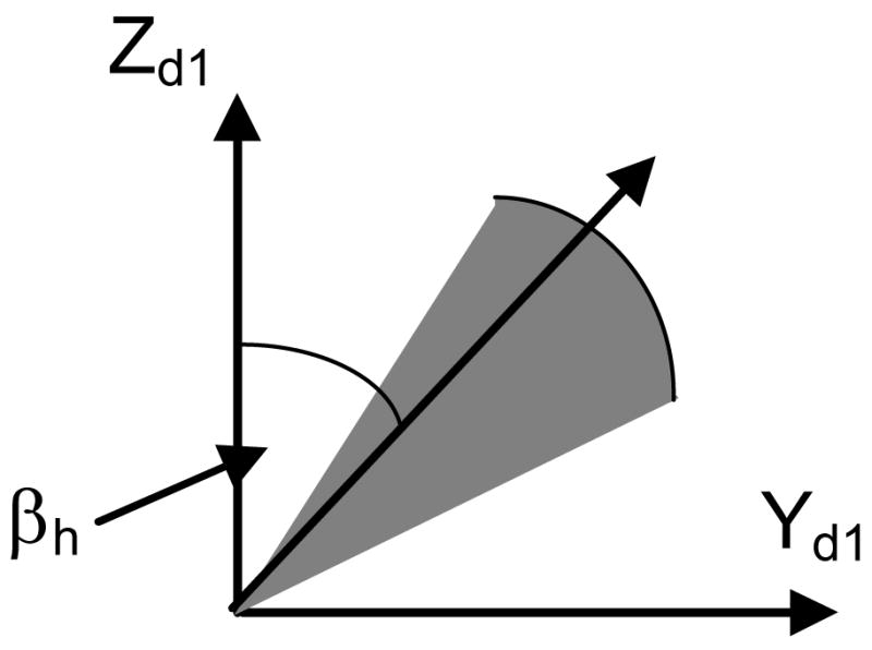
The workspace of a hinge with a limited range of rotation can be depicted as a sector with a unit radius (Fig. 4). In Fig. 4, X_h represents the orientation of the hinge axis which is determined by the ZXZ Euler angles α₀, β₀ and γ₀. The rigid-body motion at a hinge consists of only one rotation β_h about X_h.

Figure 4.

Workspace of a hinge with a limited range of rotation. (X_d1Y_d1Z_d1) represents the frame of reference at the distal end of Segment 1, (X_p2Y_p2Z_p2) represents the frame of reference at the proximal end of Segment 2. (X′Y′Z′) is an intermediate frame of reference obtained by rotating (X_d1Y_d1Z_d1) by an angle of α₀ about its Z axis followed by rotating the current frame an angle of β₀ about its X axis. (X_hY_hZ_h) is obtained by rotating (X′Y′Z′) an angle of γ₀ about its Z axis.

We notice that an arbitrarily located sector with a unit radius, as shown in Fig. 4, results from moving a sector of same area, which is inside the Y–Z plane (Fig. 5), to the new position determined by α₀, β₀ and γ₀ (Fig. 4). Therefore, in general, denoting f(β_h) as the probability distribution of the bending angle β_h at the hinge, the PDF of rigid-body motion on SE(3) at this hinge can be obtained as a convolution

Figure 5.

Workspace of a hinge constrained to move in the Y–Z plane

$$f_j(\mathbf{a},\mathbf{R}(\alpha ,\beta ,\gamma ))=(f_{j1}\ast f_{j2})(\mathbf{a},\mathbf{R}(\alpha ,\beta ,\gamma )),$$ (15)

where α ∈ [0,2π], β ∈ [0, π], and γ ∈ [0,2π], and

$$\begin{array}{l}{f}_{j1}(\mathbf{a},\mathbf{R}(\alpha ,\beta ,\gamma ))=\delta (\mathbf{R}{({\alpha }_0,{\beta }_0,{\gamma }_0)}^{-1}\mathbf{R}(\alpha ,\beta ,\gamma ))\delta (\mathbf{a})\\ =\frac{\delta (\mathbf{a})\delta (\alpha -{\alpha }_0)\delta (\beta -{\beta }_0)\delta (\gamma -{\gamma }_0)}{sin\beta },\end{array}$$ (16)

$$f_{j2}(\mathbf{a},\mathbf{R}(\alpha ,\beta ,\gamma ))=\frac{\delta (\mathbf{a})\delta (\alpha )f(\beta )\delta (\gamma )}{sin\beta }.$$ (17)

Then the Fourier transform of f_j(a,R) on SE(3) can be obtained as

$${\widehat{\mathbf{f}}}_j^r(p)={\widehat{\mathbf{f}}}_{j2}^r(p){\widehat{\mathbf{f}}}_{j1}^r(p),$$ (18)

where

$$\begin{array}{l}{\widehat{f}}_{j{1}_{l^{\prime },m^{\prime };l,m}}^r(p)={\int }_{SE(3)}{f}_{j1}(\mathbf{a},\mathbf{R}(\alpha ,\beta ,\gamma )\overline{U_{l,m;l^{\prime },m^{\prime }}^r(\mathbf{a},\mathbf{R};p)}d\mathbf{R}d\mathbf{a}\\ ={\int }_{SE(3)}\frac{\delta (\mathbf{a})\delta (\alpha -{\alpha }_0)\delta (\beta -{\beta }_0)\delta (\gamma -{\gamma }_0)}{sin\beta }\overline{U_{l,m;l^{\prime },m^{\prime }}^r(\mathbf{a},\mathbf{R};p)}d\mathbf{R}d\mathbf{a}\\ ={\int }_{SO(3)}\frac{\delta (\alpha -{\alpha }_0)\delta (\beta -{\beta }_0)\delta (\gamma -{\gamma }_0)}{sin\beta }\overline{U_{l,m;l^{\prime },m^{\prime }}^r(\mathbf{0},\mathbf{R};p)}d\mathbf{R}\\ ={\delta }_{l,l^{\prime }}{\int }_0^{2\pi }{\int }_0^{\pi }{\int }_0^{2\pi }\frac{\delta (\alpha -{\alpha }_0)\delta (\beta -{\beta }_0)\delta (\gamma -{\gamma }_0)}{sin\beta }{e}^{im\alpha }{(-1)}^{m^{\prime }-m}{P}_{m,m^{\prime }}^l(cos\beta )e^{i{m}^{\prime }\gamma }sin\beta d\alpha d\beta d\gamma \\ ={\delta }_{l,l^{\prime }}{e}^{im{\alpha }_0}{P}_{m^{\prime },m}^l(cos{\beta }_0)e^{i{m}^{\prime }{\gamma }_0},\end{array}$$ (19)

$$\begin{array}{l}{\widehat{f}}_{j{2}_{l^{\prime },m^{\prime };l,m}}^r(p)={\int }_{SE(3)}{f}_{j2}(\mathbf{a},\mathbf{R}(\alpha ,\beta ,\gamma ))\overline{U_{l,m;l^{\prime },m^{\prime }}^r(\mathbf{a},\mathbf{R};p)}d\mathbf{R}d\mathbf{a}\\ ={\int }_{SE(3)}\frac{\delta (\mathbf{a})\delta (\alpha )f(\beta )\delta (\gamma )}{sin\beta }\overline{U_{l,m;l^{\prime },m^{\prime }}^r(\mathbf{a},\mathbf{R};p)}d\mathbf{R}d\mathbf{a}\\ ={\int }_{SO(3)}\frac{\delta (\alpha )f(\beta )\delta (\gamma )}{sin\beta }\overline{U_{l,m;l^{\prime },m^{\prime }}^r(\mathbf{0},\mathbf{R};p)}d\mathbf{R}\\ ={\delta }_{l,l^{\prime }}{\int }_0^{2\pi }{\int }_{\beta }{\int }_0^{2\pi }\frac{\delta (\alpha )f(\beta )\delta (\gamma )}{sin\beta }{e}^{im\alpha }{(-1)}^{m^{\prime }-m}{P}_{m,m^{\prime }}^l(cos\beta )e^{i{m}^{\prime }\gamma }sin\beta d\alpha d\beta d\gamma \\ ={\delta }_{l,l^{\prime }}{\int }_{\beta }f(\beta )P_{m^{\prime },m}^l(cos\beta )d\beta ,\end{array}$$ (20)

where δ_i,j is the Kronecker delta function, and $P_{m,n}^l(x)$ is the generalized Legendre function ^{51, 62}.

In particular, when f(β_h) is a uniform distribution on the domain [β_h1,β_h2] with β_h1=β_c−Δβ and β_h2=β_c+Δβ, one obtains

$$f({\beta }_h)=\frac{1}{2\mathrm{\Delta }\beta },$$ (21)

$$f_{j2}(\mathbf{a},\mathbf{R}(\alpha ,\beta ,\gamma ))=\frac{\delta (\mathbf{a})\delta (\alpha )\delta (\gamma )}{2\mathrm{\Delta }\beta sin\beta },$$ (22)

$${\widehat{f}}_{j{2}_{l^{\prime },m^{\prime };l,m}}^r(p)=\frac{{\delta }_{l,l^{\prime }}}{2\mathrm{\Delta }\beta }{\int }_{{\beta }_c-\mathrm{\Delta }\beta }^{{\beta }_c+\mathrm{\Delta }\beta }{P}_{m^{\prime },m}^l(cos\beta )d\beta .$$ (23)

3.3. The ball joint

If the angular fluctuation of the macromolecular chain at an internal structure is not constrained to a plane, the local structure can be modeled as a spatial revolute joint, the ball joint (Fig. 6).

Figure 6.

Diagram of a macromolecular chain with an internal ball joint

With the rotation being parameterized using the ZXZ Euler angles, the rigid-body motion at the ball joint can be considered as consisting of a rotation α about the Z axis, followed by a rotation β about the current X axis, followed by a rotation γ about the current Z axis, with no translation in any direction. In fact, two Euler angles are enough to define the relative pose of the two segments connected by the ball joint (Fig. 7). The ball joint model applies to the macromolecular chain which has not only bending fluctuations but also twisting fluctuation at the local structure. The workspace of a ball joint with a limited range of rotation covers a certain area on the unit sphere (Fig. 7).

Figure 7.

Workspace of a ball joint with a limited range of rotation

In general, denoting the PDF of the bending angle β and the twisting angle α on the unit sphere as f(α,β), one has the corresponding PDF of rigid-body motion defined on SE(3) as

$$f_j(\mathbf{a},\mathbf{R}(\alpha ,\beta ,\gamma ))=\delta (\mathbf{a})f(\alpha ,\beta )\delta (\gamma ).$$ (24)

Then the Fourier transform of f_j(a,R) on SE(3) can be obtained as

$$\begin{array}{l}{\widehat{f}}_{j_{l^{\prime },m^{\prime };l,m}}^r(p)={\int }_{SE(3)}{f}_j(\mathbf{a},\mathbf{R}(\alpha ,\beta ,\gamma )\overline{U_{l,m;l^{\prime },m^{\prime }}^r(\mathbf{a},\mathbf{R};p)}d\mathbf{R}d\mathbf{a}\\ ={\int }_{SE(3)}\delta (\mathbf{a})f(\alpha ,\beta )\delta (\gamma )\overline{U_{l,m;l^{\prime },m^{\prime }}^r(\mathbf{a},\mathbf{R};p)}d\mathbf{R}d\mathbf{a}\\ ={\int }_{SO(3)}f(\alpha ,\beta )\delta (\gamma )\overline{U_{l,m;l^{\prime },m^{\prime }}^r(\mathbf{0},\mathbf{R};p)}d\mathbf{R}\\ ={\delta }_{l,l^{\prime }}{\int }_0^{2\pi }{\int }_{\alpha ,\beta }f(\alpha ,\beta )\delta (\gamma )e^{im\alpha }{(-1)}^{m^{\prime }-m}{P}_{m,m^{\prime }}^l(cos\beta )e^{i{m}^{\prime }\gamma }sin\beta d\alpha d\beta d\gamma \\ ={\delta }_{l,l^{\prime }}{\int }_{\alpha ,\beta }f(\alpha ,\beta )e^{im\alpha }{P}_{m^{\prime },m}^l(cos\beta )sin\beta d\alpha d\beta .\end{array}$$ (25)

In particular, let us look at the case when f(α,β) is a uniform distribution on a circular region on the unit sphere (Fig. 8). Here, we denote p_c as the position vector of the center of the circular region on the unit sphere, denote p_b as the position vector of an arbitrary point on the boundary of the circular region. α₀ and β₀ are the polar angle and the azimuthal angle of p_c. Clearly, p_c=[sinβ₀sinα₀, sinβ₀cosα₀, cosβ₀]. Since the circular region keeps a constant surface area when moving on the unit sphere, one can obtain from Fig. 9 that inside the circular region

Figure 8.

A ball joint with the uniform distribution on an arbitrary circular region on the unit sphere

Figure 9.

A ball joint with the uniform distribution on a circular region symmetric with respect to the Z axis on the unit sphere

$$f(\alpha ,\beta )=\frac{1}{2\pi (1-cos\mathrm{\Delta }\beta )},$$ (26)

and the corresponding PDF on SE(3) is

$$f_j(\mathbf{a},\mathbf{R}(\alpha ,\beta ,\gamma ))=\frac{\delta (\mathbf{a})\delta (\gamma )}{2\pi (1-cos\mathrm{\Delta }\beta )}.$$ (27)

It is clear that when the circular region is symmetric with respect to the Z axis (Fig. 9), the support of f(α,β) is defined as β ∈ [0, Δβ] and α ∈ [0,2π]. However, when the circular region moves away from the Z axis, β ∈ [β₀−Δβ, β₀+Δβ], but α ∉ [0,2π]. To find how α varies, one can obtain from the law of cosines

$${\left|\right|{\mathbf{p}}_b-{\mathbf{p}}_c\left|\right|}^2=2-2cos\mathrm{\Delta }\beta .$$ (28)

Then letting p_b=[sinβsinα, sinβcosα, cosβ], one can obtain

$$\alpha ={\alpha }_0\pm {cos}^{-1}(\frac{cos\mathrm{\Delta }\beta -cos\beta cos{\beta }_0}{sin\beta sin{\beta }_0}),$$ (29)

which gives the upper and lower bounds of α corresponding to any specific value of β.

Then the Fourier transform of f_j(a,R) on SE(3) can be obtained as

$$\begin{array}{l}{\widehat{f}}_{j_{l^{\prime },m^{\prime };l,m}}^r(p)=\frac{{\delta }_{l,l^{\prime }}}{2\pi (1-cos\mathrm{\Delta }\beta )}{\int }_{{\beta }_0-\mathrm{\Delta }\beta }^{{\beta }_0+\mathrm{\Delta }\beta }{\int }_{{\alpha }_0-{cos}^{-1}(\frac{cos\mathrm{\Delta }\beta -cos\beta cos{\beta }_0}{sin\beta sin{\beta }_0})}^{{\alpha }_0+{cos}^{-1}(\frac{cos\mathrm{\Delta }\beta -cos\beta cos{\beta }_0}{sin\beta sin{\beta }_0})}{e}^{im\alpha }{P}_{m^{\prime },m}^l(cos\beta )sin\beta d\alpha d\beta \\ =\frac{{\delta }_{l,l^{\prime }}}{2\pi m(1-cos\mathrm{\Delta }\beta )i}{\int }_{{\beta }_0-\mathrm{\Delta }\beta }^{{\beta }_0+\mathrm{\Delta }\beta }(e^{im({\alpha }_0+{cos}^{-1}(\frac{cos\mathrm{\Delta }\beta -cos\beta cos{\beta }_0}{sin\beta sin{\beta }_0}))}-e^{im({\alpha }_0-{cos}^{-1}(\frac{cos\mathrm{\Delta }\beta -cos\beta cos{\beta }_0}{sin\beta sin{\beta }_0}))})P_{m^{\prime },m}^l(cos\beta )sin\beta d\beta \end{array}$$ (30)

In fact, f_j(a,R) for the uniform ball joint can also be obtained using the convolution on SE(3). We notice that a circular region arbitrarily located on the unit sphere results from moving a circular region with the same radius, which is symmetric to the Z axis (Fig. 9), to the new position determined by α₀ and β₀ (Fig. 8). Therefore, the PDF of rigid-body motion on SE(3) at this ball joint can be obtained as a convolution

$$f_j(\mathbf{a},\mathbf{R}(\alpha ,\beta ,\gamma ))=(f_{j1}\ast f_{j2})(\mathbf{a},\mathbf{R}(\alpha ,\beta ,\gamma )),$$ (31)

where

$$\begin{array}{l}{f}_{j1}(\mathbf{a},\mathbf{R}(\alpha ,\beta ,\gamma ))=\delta (\mathbf{a})\delta (\mathbf{R}{({\alpha }_0,{\beta }_0,0)}^{-1}\mathbf{R}(\alpha ,\beta ,\gamma ))\\ =\frac{\delta (\mathbf{a})\delta (\alpha -{\alpha }_0)\delta (\beta -{\beta }_0)\delta (\gamma )}{sin\beta },\end{array}$$ (32)

$$f_{j2}(\mathbf{a},\mathbf{R}(\alpha ,\beta ,\gamma ))=\frac{\delta (\mathbf{a})\delta (\gamma )}{2\pi (1-cos\mathrm{\Delta }\beta )}.$$ (33)

Then the Fourier transform of f_j(a,R) on SE(3) can be obtained as

$${\widehat{\mathbf{f}}}_j^r(p)={\widehat{\mathbf{f}}}_{j2}^r(p){\widehat{\mathbf{f}}}_{j1}^r(p),$$ (34)

where

$$\begin{array}{l}{\widehat{f}}_{j{1}_{l^{\prime },m^{\prime };l,m}}^r(p)={\int }_{SE(3)}{f}_{j1}(\mathbf{a},\mathbf{R}(\alpha ,\beta ,\gamma )\overline{U_{l,m;l^{\prime },m^{\prime }}^r(\mathbf{a},\mathbf{R};p)}d\mathbf{R}d\mathbf{a}\\ ={\int }_{SE(3)}\frac{\delta (\mathbf{a})\delta (\alpha -{\alpha }_0)\delta (\beta -{\beta }_0)\delta (\gamma )}{sin\beta }\overline{U_{l,m;l^{\prime },m^{\prime }}^r(\mathbf{a},\mathbf{R};p)}d\mathbf{R}d\mathbf{a}\\ ={\int }_{SO(3)}\frac{\delta (\alpha -{\alpha }_0)\delta (\beta -{\beta }_0)\delta (\gamma )}{sin\beta }\overline{U_{l,m;l^{\prime },m^{\prime }}^r(\mathbf{0},\mathbf{R};p)}d\mathbf{R}\\ ={\delta }_{l,l^{\prime }}{\int }_0^{2\pi }{\int }_0^{\pi }{\int }_0^{2\pi }\frac{\delta (\alpha -{\alpha }_0)\delta (\beta -{\beta }_0)\delta (\gamma )}{sin\beta }{e}^{im\alpha }{(-1)}^{m^{\prime }-m}{P}_{m,m^{\prime }}^l(cos\beta )e^{i{m}^{\prime }\gamma }sin\beta d\alpha d\beta d\gamma \\ ={\delta }_{l,l^{\prime }}{e}^{im{\alpha }_0}{P}_{m^{\prime },m}^l(cos{\beta }_0),\end{array}$$ (35)

$$\begin{array}{l}{\widehat{f}}_{2l^{\prime },m^{\prime };l,m}^r(p)={\int }_{SE(3)}{f}_{j2}(\mathbf{a},\mathbf{R}(\alpha ,\beta ,\gamma )\overline{U_{l,m;l^{\prime },m^{\prime }}^r(\mathbf{a},\mathbf{R};p)}d\mathbf{R}d\mathbf{a}\\ ={\int }_{SE(3)}\frac{\delta (\mathbf{a})\delta (\gamma )}{2\pi (1-cos\mathrm{\Delta }\beta )}\overline{U_{l,m;l^{\prime },m^{\prime }}^r(\mathbf{a},\mathbf{R};p)}d\mathbf{R}d\mathbf{a}\\ ={\int }_{SO(3)}\frac{\delta (\gamma )}{2\pi (1-cos\mathrm{\Delta }\beta )}\overline{U_{l,m;l^{\prime },m^{\prime }}^r(\mathbf{0},\mathbf{R};p)}d\mathbf{R}\\ ={\delta }_{l,l^{\prime }}{\int }_0^{2\pi }{\int }_0^{\mathrm{\Delta }\beta }{\int }_0^{2\pi }\frac{\delta (\gamma )}{2\pi (1-cos\mathrm{\Delta }\beta )}{e}^{im\alpha }{(-1)}^{m^{\prime }-m}{P}_{m,m^{\prime }}^l(cos\beta )e^{i{m}^{\prime }\gamma }sin\beta d\alpha d\beta d\gamma \\ =\frac{{\delta }_{l,l^{\prime }}{\delta }_{m,0}}{1-cos\mathrm{\Delta }\beta }{\int }_0^{\mathrm{\Delta }\beta }{P}_{m^{\prime },0}^l(cos\beta )sin\beta d\beta .\end{array}$$ (36)

4. The PDF of the end-to-end distance for the rigid chain with an internal joint

As mentioned before, the PDF of end-to-end distance is of particular interest, and is a marginal density of the full PDF of end-to-end pose. Moreover, when the macromolecular chain is completely rigid, it is possible to derive the closed form solution for the PDF of the end-to-end distance. In this section, we take a look at the case of two rigid rods connected by a joint (Fig. 10). Our method can easily be extended to the multi-joint case by using geometric relationships.

Figure 10.

Diagram of two rigid rods connected by a joint

In general, knowing the PDF of the bending angle, p(β), one can derive the PDF of the end-to-end distance, f(a), from the following relationship

$$f(a)=p(\beta )\mid \frac{d\beta }{da}\mid ,$$ (37)

where

$$\frac{d\beta }{da}=-\frac{2a}{\sqrt{({(L_1+L_2)}^2-a^2)(a^2-{(L_1-L_2)}^2)}}.$$ (38)

Equation (38) can be derived from

$$a^2={L_1}^2+{L_2}^2-2L_1{L}_{2}cos(\pi -\beta ),$$ (39)

which is obtained from the law of cosine.

When the joint is a hinge with a limited range of rotation, one can obtain from Fig. 4

$$cos\beta =-sin{\beta }_{0}cos{\gamma }_{0}sin{\beta }_h+cos{\beta }_{0}cos{\beta }_h,$$ (40)

from which one can further obtain

$$p(\beta )=f({\beta }_h)\mid \frac{d{\beta }_h}{d\beta }\mid =\frac{k_1({\beta }_h)}{k_2({\beta }_h)}f({\beta }_h),$$ (41)

where

$$k_1({\beta }_h)=\sqrt{1-{(-sin{\beta }_{0}cos{\gamma }_{0}sin{\beta }_h+cos{\beta }_{0}cos{\beta }_h)}^2},$$ (42)

$$k_2({\beta }_h)=\mid sin{\beta }_{0}cos{\gamma }_{0}cos{\beta }_h+cos{\beta }_{0}sin{\beta }_h\mid .$$ (43)

Substituting (41) into (37), one obtains

$$f(a)=\frac{2a{k}_1({\beta }_h(a))}{k_2({\beta }_h(a))\sqrt{({(L_1+L_2)}^2-a^2)(a^2-{(L_1-L_2)}^2)}}f({\beta }_h(a)),$$ (44)

where

$${\beta }_h(a)={cos}^{-1}(\frac{k_3(a)cos{\beta }_0\pm \sqrt{k_3{(a)}^2{cos}^2{\beta }_0-({cos}^2{\beta }_0+{sin}^2{\beta }_0{cos}^2{\gamma }_0)(k_3{(a)}^2-{sin}^2{\beta }_0{cos}^2{\gamma }_0)}}{{cos}^2{\beta }_0+{sin}^2{\beta }_0{cos}^2{\gamma }_0}),$$ (45)

$$k_3(a)=\frac{a^2-{L_1}^2-{L_2}^2}{2L_1{L}_2}.$$ (46)

In particular, when f(β_h) is a uniform distribution on the domain [β_c− Δβ,β_c+Δβ], one obtains

$$f(a)=\frac{a{k}_1({\beta }_h(a))}{\mathrm{\Delta }\beta k_2({\beta }_h(a))\sqrt{({(L_1+L_2)}^2-a^2)(a^2-{(L_1-L_2)}^2)}}.$$ (47)

When the joint is a ball joint with a limited range of rotation, and f(α,β) is a uniform distribution on a circular region of the unit sphere, one obtains from (33)

$$\begin{array}{l}p(\beta )={\int }_{{\alpha }_0-{cos}^{-1}(\frac{cos\mathrm{\Delta }\beta -cos\beta cos{\beta }_0}{sin\beta sin{\beta }_0})}^{{\alpha }_0+{cos}^{-1}(\frac{cos\mathrm{\Delta }\beta -cos\beta cos{\beta }_0}{sin\beta sin{\beta }_0})}\frac{sin\beta }{2\pi (1-cos\mathrm{\Delta }\beta )}d\alpha \\ =\frac{sin\beta {cos}^{-1}(\frac{cos\mathrm{\Delta }\beta -cos\beta cos{\beta }_0}{sin\beta sin{\beta }_0})}{\pi (1-cos\mathrm{\Delta }\beta )}.\end{array}$$ (48)

Substituting (48) into (37), one obtains

$$f(a)=\frac{a{cos}^{-1}(\frac{2L_1{L}_{2}cos\mathrm{\Delta }\beta -(a^2-{L_1}^2-{L_2}^2)cos{\beta }_0}{\sqrt{({(L_1+L_2)}^2-a^2)(a^2-{(L_1-L_2)}^2)}sin{\beta }_0}}{\pi L_1{L}_2(1-cos\mathrm{\Delta }\beta )}.$$ (49)

5. Examples and discussion

In this section, we will show how to implement our method derived in the last two sections by examples. We will present our results in the form of f(a) instead of f(a,R) for the convenience of display, though f(a,R) contains more information than f(a) and can be obtained using our methods.

The general formulation reviewed in Section 2 applies to several stiffness models. Here we use the Kratky-Porod model in our examples. However, other models, such as the Yamakawa model and the Marko-Siggia model, also fit into our general formulation. For the Kratky-Porod wormlike chain model, the stiffness matrix, chirality vector and constant term in (2) are defined as ²⁸

$$\mathbf{B}=\left(\begin{array}{ccc}\chi & 0& 0\\ 0& \chi & 0\\ 0& 0& 0\end{array}\right),\mathbf{b}=\left(\begin{array}{c}0\\ 0\\ 0\end{array}\right),\text{c}=0,$$ (50)

where χ is known as the stiffness parameter. The definitions of the stiffness matrix, chirality vector and constants for the Yamakawa model and Marko-Siggia models can be found in ²⁸. In our computation, the stiffness is measured in units of k_BT. Moreover, all the stiffness and length parameters are normalized by the total arclength of the macromolecular chain.

When implementing the Fourier transform for SE(3), by definition (as shown in equation (7)), r∈Z, p∈[0,∞], and B^r is an infinite dimensional matrix. To do numerical computations, however, one must truncate r, l, l′, and p at finite values, and B^r at finite dimension. In particular, when f(a) is of interest, we only need to consider r=0, as suggested by (13).

As shown in Fig. 11, we compute f(a) of a macromolecular chain with a limited uniform hinge in the middle under different values of stiffness. In this example, we choose the range of rotation as β_h∈[π/3, 2π/3] with α₀=β₀=γ₀=0. The choices of the computation parameters are listed in Table 1, where r∈[−l_b, l_b], l∈[r, l_b], l′∈[r, l_b], and p∈[0,p_b].

Figure 11.

Variation of the PDF of the end-to-end distance of a macromolecular chain with a limited hinge in the middle with respect to the stiffness

Table 1.

Values of computation parameters used in the hinge example

χ	lb	pb
0.1	3	50
0.2	4	60
0.3	4	80
0.4	5	80
0.5	5	100
1.0	7	130
2.0	11	150
3.0	13	150
4.0	16	190
5.0	18	200

As shown in Fig. 12, we compute f(a) for a macromolecular chain with a limited uniform ball joint in the middle under different values of stiffness. In this example, we choose the range of rotation as a circular region on the unit sphere centered at α₀=β₀=π/2 with Δβ=π/6. The choices of the computation parameters are listed in Table 2, where r∈[−l_b, l_b], l∈[r, l_b], l′∈[r, l_b], and p∈[0,p_b].

Figure 12.

Variation of the PDF of the end-to-end distance of a macromolecular chain with a limited ball joint in the middle with respect to the stiffness

Table 2.

Values of computation parameters used in the ball joint example

χ	lb	pb
0.1	3	50
0.2	4	70
0.3	4	80
0.4	5	80
0.5	5	100
1.0	7	130
2.0	11	180
3.0	13	170
4.0	16	190

It is clear from our examples that given the type of the joint and the range of rotation, the macromolecular chains with different values of stiffness will have different PDFs of end-to-end distance. This means that one can determine the stiffness of a macromolecular chain with a known internal joint from the experimentally-measured PDF. Meanwhile, knowing the stiffness of a macromolecular chain with an internal joint, it is also possible to distinguish between hinge-like and ball-like joints from experimentally-measured PDFs. From our computation, we notice that the difference between the PDF of a macromolecular chain with a hinge and that of a chain with a ball joint is small when the stiffness is low, and increases as the stiffness gets higher (Fig. 13). Therefore, it would be easier to identify the type of the joint from experimentally obtained end-to-end distance distributions for a stiffer macromolecular chain than that for a more flexible chain.

Figure 13.

Root-mean-square difference between the PDF of the hinge example and that of the ball joint example. e(χ) denotes the root-mean-square difference between the PDF of the hinge case and that of the ball joint case. It is defined as $e(\chi )=\sqrt{{\int }_0^1{(f_{\mathit{hinge}}(a,\chi )-f_{\mathit{ball}}(a,\chi ))}^{2}da}$. In the case of the rigid chain with a joint in the middle (χ=∞, which is not shown on the plot), e(χ=∞)≈0.55.

A variety of experimental methods can be used to directly measure the end-to-end distance of a macromolecular chain and generate the PDF of the end-to-end distance. Single molecule FRET is the most widely adopted way to study the conformational distribution and dynamics of individual macromolecules, which efficiently measures the intramolecular distances from 3nm to 10nm ^63–66. At the low end, fluorescence quenching by TEMPO measures the sub-3nm distances with a resolution of 0.5nm ⁶³, and a single-molecule optical switch based on Cy5 and Cy3 can measure the intramolecular distances as short as 1nm ⁶⁴. At the high end, a molecular ruler based on plasmon coupling of single gold and silver particles can measure intermolecular distances continuously up to 70nm ⁶⁵. Meanwhile, single-molecule high-resolution colocalization (SHREC) of fluorescent probes can measure the intramolecular distances from 10nm to 200nm over time, and has been used to generate the distribution of the end-to-end distance of DNA fragments ⁶⁶. Besides these distance-measuring methods, the distribution of the end-to-end distance of a free macromolecular chain can also be retrieve from the force-extension experiments ^{67, 68}. By holding different end-to-end distances and measuring the average holding forces, one can establish a force-extension relation and retrieve the distribution of the end-to-end distance based on $<F>=-\frac{\partial log(f(a))}{\partial a}$, where <F> denotes the average holding force ⁶⁷. The holding experiment can be implemented by laser trap and atomic force microscopy ⁶⁸.

In addition to these direct measurement techniques, indirect methods that measure moments of the end-to-end distance distribution also exist. The following section discusses how the radius of gyration for semiflexible chains with internal defects (which can be computed from our model) relates to light-scattering experiments.

6. Detecting joints in semiflexible chains based on radius of gyration

The proposed method also provides a potential tool for detecting the existence of joint-like internal structures in single macromolecular chains based on the radius of gyration measured from the laser light scattering experiment, which achieves a precision of 2–4% ^69–71.

In principle, the radius of gyration of a chain with internal joints will be different from that of an intrinsically straight chain. For a single macromolecular chain, one can measure the radius of gyration from the light scattering experiment. One can also compute the radius of gyration of a comparable intrinsically straight chain with same stiffness. By comparing the measured radius of gyration with the calculated one, one can determine if there is a joint-like internal structure on the chain.

To study the feasibility of detecting the existence of internal joints on single macromolecular chains based on the radius of gyration, we compute and compare the radius of gyration of both intrinsically straight chain and jointed chain based on the PDFs generated by the proposed method. Here we use the macromolecular chain with a limited hinge in the middle as our example of the jointed chain, with α₀=β₀=γ₀=0 and β_h ∈ [β−Δβ, β+Δβ]. β is the central bending angle at the hinge, and Δβ is the half-range angle. Denoting the radius of gyration as R_G, we will study the impact of both β and Δβ on R_G.

The radius of gyration of a single macromolecular chain can be computed from the PDFs of its point-to-point distances. Discretizing a chain into n segments, one can calculate the radius of gyration as ⁷²

$$R_G=\frac{\sqrt{{\displaystyle \sum _{j=1}^n}{\displaystyle \sum _{i=1}^n}<{r_{ij}}^2>}}{\sqrt{2}n},$$ (51)

where

$$<r_{ij}^2>={\int }_0^{l_{ij}}{r}_{ij}^2{f}_{ij}(r_{ij}){dr}_{ij}.$$ (52)

Here, r_ij denotes the distance between two points i and j on the chain, l_ij denotes the arclength between i and j, and f_ij(r_ij) denotes the PDF of the distance between i and j which can be generated using the method presented in previous sections. Equ.51 applies to both intrinsically straight and jointed chains.

In Fig. 14 and Fig. 15, we study the impact of Δβ on R_G, with β=0. In this case, the jointed chain fluctuates around a straight conformation. A DNA with a symmetric internal loop belongs to this category.

Figure 14.

Comparison in R_G between the intrinsically straight and hinged macromolecular chains with β =0 and different Δβ

Figure 15.

Difference in R_G between the intrinsically straight chain and the hinged chains with β=0 and different Δβ. Here, ΔR_G=R_Gs − R_Gh where R_Gs denotes the radius of gyration of the intrinsically straight chain, and R_Gh denotes the radius of gyration of the hinged chain. Fig. 15a presents the difference in absolute value, and Fig. 15b presents the difference in percentage.

By changing χ, we obtain a class of R_G -χ curves for the intrinsically straight chain and the jointed chains with different Δβ. Fig. 14 shows that in general,

1. R_G of a jointed chain is smaller than that of an intrinsically straight chain with same stiffness, because the joint causes the chain to fold back.

2. R_G of a flexible chain is small, because the conformation of such a chain is usually an entangled coil.

3. R_G of the chain increases as χ increases, because the conformation of a stiffer chain tends to stretch out. Moreover, a stiffer chain behaves more like a rigid chain. Therefore R_G of a jointed chain converges to that of the rigid chain as χ increases.

4. R_G of a jointed chain with a larger Δβ tends to be smaller, because such a chain is more likely to fold back.

The difference in R_G between the intrinsically straight chain and the jointed chains with β=0 and different Δβ is presented in Fig. 15.

Fig. 15 shows that ΔR_G increases as Δβ increases. This means that an internal joint with a larger fluctuation range is more distinguishable from the intrinsically straight chain. Table 3 presents the percentage difference of R_G, when χ=1, between the intrinsically straight chain and the jointed chains with zero β. The table shows that a jointed chain with Δβ≥π/2 is highly detectable based on the experimentally-measured R_G, according to the reported measurement precision ^69–71.

Table 3.

Percentage difference in R_G between the straight chain and the jointed chains with zero β (χ=1)

Δβ	π/6	π/3	π/2	2π/3	5π/6	π
ΔRG/RGh*100%	0.64%	2.88%	6.55%	11.40%	16.98%	22.52%

In Fig. 16 and Fig. 17, we study the impact of β on R_G, with Δβ=π/6. In this case, the jointed chain fluctuates around a bent conformation. A DNA with a bulge or a gap belongs to this category.

Figure 16.

Comparison in R_G between the intrinsically straight and hinged macromolecular chains with Δβ = π/6 and different β

Figure 17.

Difference in R_G between the intrinsically straight chain and the hinged chains with Δβ=π/6 and different β. Fig. 17a presents the difference in absolute value, and Fig. 17b presents the difference in percentage.

By changing χ, we obtain a class of R_G -χ curves for the intrinsically straight chain and the jointed chains with different β. Fig. 16 shows a similar relation between R_G and χ as Fig. 14 does. Moreover, R_G of a jointed chain with a larger β tends to be smaller, because β forces the chain to fold back.

The difference in R_G between the intrinsically straight chain and the jointed chains with Δβ=π/6 and different β is presented in Fig. 17.

Fig. 17 shows that ΔR_G increases as β increases. This means that an internal joint with a larger bending is more distinguishable from the intrinsically straight chain. Table 4 presents the percentage difference of R_G, when χ=1, between the intrinsically straight chain and the jointed chains with Δβ=π/6. The table shows that a jointed chain with β≥π/4 is highly detectable based on the experimentally-measured R_G, according to the reported measurement precision ^69–71.

Table 4.

Percentage difference in R_G between the straight chain and the jointed chains with Δβ=π/6 (χ=1)

β	π/6	π/4	π/3	π/2	2π/3	5π/6	π
ΔRG/RGh*100%	2.98%	5.93%	10.17%	22.89%	41.28%	61.45%	71.13%

Fig. 18 shows the combined effect of both β and Δβ on R_G. In general, a jointed chain with larger β and/or Δβ is more distinguishable from the intrinsically straight chain.

Figure 18.

Difference in R_G between the intrinsically straight chain and the hinged chains with different β and Δβ. Fig. 18a shows the contour plot of the percentage difference when χ=1, and Fig. 18b shows the contour plot of the percentage difference when χ=2.

7. Conclusion

In this paper, we proposed an effective computational method to estimate the conformational statistics of semi-flexible macromolecular chains with internal structures which can be represented as joints with limited capability of rotation, such as DNAs containing symmetric loops, bulges, and nicks/gaps. Our method can compute the PDF of the end-to-end pose of a macromolecular chain with any stiffness and chirality in its minimum energy states. Other marginal PDFs and statistical quantities can be further calculated from this full PDF. The proposed method extends our previous general formulation of classical polymer theory, and can be used with different stiffness models, including the Krathy-Porod model, Yamakawa model and the Marko-Siggia model. This capability allows one to study the entropic effects of internal angular fluctuations on semi-flexible macromolecular chains with internal joints. Our method also provides a potential tool to detect the existence of internal joints. With the complete spectrum of computational results obtained using this method, it is possible in principle to retrieve the stiffness, joint type and joint location of a macromolecular chain with an internal defect from experimentally-measured PDFs. The current method ignores the interactions among the segments of the same macromolecular chain. This will become a topic of our future work.

References

- 1.Marini JC, Levene SD, Crothers DM, Englund PT. Proceedings of the National Academy of Sciences of the USA- Biological Sciences. 1982;79:7664–7668. doi: 10.1073/pnas.79.24.7664. [DOI] [PMC free article] [PubMed] [Google Scholar]
- 2.Van der Vliet PC, Verrijzer CP. Bioessays. 1993;15:25–32. doi: 10.1002/bies.950150105. [DOI] [PubMed] [Google Scholar]
- 3.Perez-Martin J, Rojo F, De Lorenzo V. Microbiological Review. 1994;58:268–290. doi: 10.1128/mr.58.2.268-290.1994. [DOI] [PMC free article] [PubMed] [Google Scholar]
- 4.Dickerson RE, Goodsell D, Kopka ML. Journal of Molecular Biology. 1996;256:108–125. doi: 10.1006/jmbi.1996.0071. [DOI] [PubMed] [Google Scholar]
- 5.Hansma HG, Browne KA, Bezanilla M, Bruice TC. Biochemstry. 1994;33:8436–8441. doi: 10.1021/bi00194a007. [DOI] [PubMed] [Google Scholar]
- 6.Griffith J, Bleyman M, Rauch CA, Kitchin PA, Englund PT. Cell. 1986;46:717–724. doi: 10.1016/0092-8674(86)90347-8. [DOI] [PubMed] [Google Scholar]
- 7.Crothers DM, Haran TE, Nadeau JG. Journal of Biological Chemistry. 1990;265:7093–7096. [PubMed] [Google Scholar]
- 8.Benoff B, Yang H, Lawson CL, Parkinson G, Liu J, Blatter E, Ebright YW, Berman HM, Ebright RH. Science. 2002;297:1562–1566. doi: 10.1126/science.1076376. [DOI] [PubMed] [Google Scholar]
- 9.Guo H, Tullius TD. Proceedings of the National Academy of Sciences of the United States of America. 2003;100:3743–3747. doi: 10.1073/pnas.0737062100. [DOI] [PMC free article] [PubMed] [Google Scholar]
- 10.Roll C, Ketterle C, Faibis V, Fazakerley GV, Boulard Y. Biochemistry. 1998;37:4059–4070. doi: 10.1021/bi972377w. [DOI] [PubMed] [Google Scholar]
- 11.Kahn JD, Yun E, Crothers DM. Nature. 1994;368:163–166. doi: 10.1038/368163a0. [DOI] [PubMed] [Google Scholar]
- 12.Zacharias M, Hagerman PJ. Journal of Molecular Biology. 1996;257:276–289. doi: 10.1006/jmbi.1996.0162. [DOI] [PubMed] [Google Scholar]
- 13.Gohlke C, Murchie AIH, Lilley DMJ, Clegg RM. Proceedings of the National Academy of Sciences of the United States of America. 1994;91:11660–11664. doi: 10.1073/pnas.91.24.11660. [DOI] [PMC free article] [PubMed] [Google Scholar]
- 14.Luebke KJ, Landry SM, Tinoco I. Biochemistry. 1997;36:10246–10255. doi: 10.1021/bi9701540. [DOI] [PubMed] [Google Scholar]
- 15.Dornberger U, Hillisch A, Gollmick FA, Fritzsche H, Diekmann S. Biochemistry. 1999;38:12860–12868. doi: 10.1021/bi9906874. [DOI] [PubMed] [Google Scholar]
- 16.Zacharias M, Hagerman PJ. Journal of Molecular Biology. 1995;247:486–500. doi: 10.1006/jmbi.1995.0155. [DOI] [PubMed] [Google Scholar]
- 17.Luebke KL, Tinoco I. Biochemistry. 1996;35:11677–11684. doi: 10.1021/bi960914r. [DOI] [PubMed] [Google Scholar]
- 18.Gollmick FA, Lorenz M, Dornberger U, von Langen J, Diekmann S, Fritzsche H. Nucleic Acids Research. 2002;30:2669–2677. doi: 10.1093/nar/gkf375. [DOI] [PMC free article] [PubMed] [Google Scholar]
- 19.Feig M, Zacharias M, Pettitt BM. Biophysical Journal. 2001;81:352–370. doi: 10.1016/S0006-3495(01)75705-0. [DOI] [PMC free article] [PubMed] [Google Scholar]
- 20.Zacharias M, Sklenar H. Biophysical Journal. 2000;78:2528–2542. doi: 10.1016/S0006-3495(00)76798-1. [DOI] [PMC free article] [PubMed] [Google Scholar]
- 21.Flory PJ. Statistical Mechanics of Chain Molecules. Interscience Publishers; New York: 1969. [Google Scholar]
- 22.Kratky O, Porod G. Recueil Des Travaux Chimiques Des Pays-Bas. 1949;68:1106–1122. [Google Scholar]
- 23.Daniels HE. Proceedings of the Royal Society of Edinburgh. 1952;A 63:290–311. [Google Scholar]
- 24.Hermans JJ, Ullman R. Physica. 1952;18:951–971. [Google Scholar]
- 25.Yamakawa H. Helical Wormlike Chains in Polymer Solutions. Springer; New York: 1997. [Google Scholar]
- 26.Marko JF, Siggia ED. Macromolecules. 1994;27:981–988. [Google Scholar]
- 27.Zhou H, Ou-Yang Z. Physical Review E. 1998;58:4816–4819. [Google Scholar]
- 28.Chirikjian GS, Wang Y. Physics Review E. 2000;62:880–892. doi: 10.1103/physreve.62.880. [DOI] [PubMed] [Google Scholar]
- 29.Fixman M, Alben R. Journal of Chemical Physics. 1973;58:1553–1558. [Google Scholar]
- 30.Maroun RC, Olson WK. Biopolymers. 1988;27:561–584. doi: 10.1002/bip.360270403. [DOI] [PubMed] [Google Scholar]
- 31.Hagerman PJ. Biopolymers. 1985;24:1881–1897. doi: 10.1002/bip.360241004. [DOI] [PubMed] [Google Scholar]
- 32.Lax M, Barrett AJ, Domb C. Journal of Physics A-Mathematical and General. 1978;11:361–374. [Google Scholar]
- 33.Croxton C. A Journal of Physics A-Mathematical and General. 1979;12:2475–2485. [Google Scholar]
- 34.Nitta KH. Journal of Chemical Physics. 1994;101:4222–4228. [Google Scholar]
- 35.Aguileragranja F, Kkuchi R. Physica A. 1992;182:331–345. [Google Scholar]
- 36.Liao Q, Wu DC. ACTA Polymerica SINCA. 2000;4:420–425. [Google Scholar]
- 37.Wu DC, Du P, Kang J. Science in China Series B-Chemistry. 1997;40:137–145. [Google Scholar]
- 38.Liverpool TB, Edwards SF. Journal of Chemical Physics. 1995;103:6716–6719. [Google Scholar]
- 39.Walasek J. Journal of Polymer Science Part B-Polymer Physics. 1988;26:1907–1922. [Google Scholar]
- 40.Burlatskii SF, Oshanin GS. Theoretical and Mathematical Physics. 1998;75:659–663. [Google Scholar]
- 41.Coriell SR, Jackson JL. Journal of Mathematical Physics. 1967;8:1276. [Google Scholar]
- 42.Kosmas MK. Journal of Physics A-Mathematical and General. 1983;16:L381–L384. [Google Scholar]
- 43.Wilhelm J, Frey E. Physical Review Letters. 1996;77:2581–2584. doi: 10.1103/PhysRevLett.77.2581. [DOI] [PubMed] [Google Scholar]
- 44.Lagowski JB, Noolandi J, Nickel B. Journal of Chemical Physics. 1991;95:1266–1269. [Google Scholar]
- 45.Ronca G, Yoon DY. Journal of Chemical Physics. 1984;80:930–935. [Google Scholar]
- 46.Mondescu RP, Muthukumar M. Physical Review E. 1998;57:4411–4419. [Google Scholar]
- 47.Mondescu RP, Muthukumar M. Journal of Chemical Physics. 1999;110:12240–12249. [Google Scholar]
- 48.Hoffman GG. Journal of Physical Chemistry B. 1999;103:7167–7174. [Google Scholar]
- 49.Papadopoulos GJ, Thomchick J. Journal of Physics A- Mathematical and General. 1977;10:1115–1121. [Google Scholar]
- 50.Dua A, Cherayil BJ. Journal of Chemical Physics. 1998;109:7011–7016. [Google Scholar]
- 51.Chirikjian GS, Kyatkin AB. Engineering Applications of Noncommutative Harmonic Analysis. CRC Press; Boca Raton, FL: 2000. [Google Scholar]
- 52.Chirikjian GS, Kyatkin AB. Journal of Fourier Analysis and Applications. 2000;6:583–606. [Google Scholar]
- 53.Chirikjian GS. Computational and Theoretical Polymer Science. 2001;11:143–153. [Google Scholar]
- 54.Hagerman PJ. Annual Review of Biochemistry. 1990;59:755–781. doi: 10.1146/annurev.bi.59.070190.003543. [DOI] [PubMed] [Google Scholar]
- 55.Hagerman PJ. Biochimica et Biophysica Acta. 1992;1131:125–132. doi: 10.1016/0167-4781(92)90066-9. [DOI] [PubMed] [Google Scholar]
- 56.Olson WK, Zhurkin VB. Biological Structure and Dynamics. Proceedings of the Ninth Conversation in the Discipline Biomolecular Stereodynamics; 1996. pp. 341–370. [Google Scholar]
- 57.Olson WK, Marky NL, Jernigan RL, Zhurkin VB. Journal of Molecular Biology. 1993;232:530–551. doi: 10.1006/jmbi.1993.1409. [DOI] [PubMed] [Google Scholar]
- 58.Rivetti C, Walker C, Bustamante C. Journal of Molecular Biology. 1998;280:41–59. doi: 10.1006/jmbi.1998.1830. [DOI] [PubMed] [Google Scholar]
- 59.Zhou Y, Chirikjian GS. Journal of Chemical Physics. 2003;119:4962–4970. [Google Scholar]
- 60.Kyatkin AB, Chirikjian GS. Applied and Computational Harmonic Analysis. 2000;9:220–241. [Google Scholar]
- 61.Miller W. Communications on Pure and Applied Mathematics. 1964;17:527–540. [Google Scholar]
- 62.Vilenkin NJ, Klimyk AU. Representation of Lie Groups and Special Functions. Kluwer Academic Publishers; Dordrecht, Holland: 1991. [Google Scholar]
- 63.Zhu P, Clamme J, Deniz AA. Biophysical Journal: Biophysical Letters. 2005:L37–L39. doi: 10.1529/biophysj.105.071027. [DOI] [PMC free article] [PubMed] [Google Scholar]
- 64.Bates M, Blosser TR, Zhuang X. Physical Review Letters. 2005;94:108101.1–4. doi: 10.1103/PhysRevLett.94.108101. [DOI] [PMC free article] [PubMed] [Google Scholar]
- 65.Sonnichsen C, Reinhard BM, Liphardt J, Alivisatos AP. Nature Biotechnology. 2005;23:741–745. doi: 10.1038/nbt1100. [DOI] [PubMed] [Google Scholar]
- 66.Churchman LS, Okten Z, Rock RS, Dawson JF, Spudich JA. Proceedings of the National Academy of Sciences of the United States of America. 2005;102:1419–1423. doi: 10.1073/pnas.0409487102. [DOI] [PMC free article] [PubMed] [Google Scholar]
- 67.Ranjith P, Kumar PBS, Menon G. Physical Review Letters. 2005;94:138102.1–4. doi: 10.1103/PhysRevLett.94.138102. [DOI] [PubMed] [Google Scholar]
- 68.Keller D, Swigon D, Bustamante C. Biophysical Journal. 2003;84:733–738. doi: 10.1016/S0006-3495(03)74892-9. [DOI] [PMC free article] [PubMed] [Google Scholar]
- 69.Lai E, Zanten JHV. Biophysical Journal. 2001;80:864–873. doi: 10.1016/S0006-3495(01)76065-1. [DOI] [PMC free article] [PubMed] [Google Scholar]
- 70.Zhou H, Miller AW, Sosic Z, Buchholz B, Barron AE, Kotler L, Karger BL. Analytical Chemistry. 2000;72:1045–1052. doi: 10.1021/ac991117c. [DOI] [PubMed] [Google Scholar]
- 71.Jeng L, Balke ST, Mourey TH, Wheeler L, Romeo P. Journal of Applied Polymer Science (USA) 1993;49:1359–1374. [Google Scholar]
- 72.Johnson CS, Gabriel DA. Laser Light Scattering. Dover; 1994. [Google Scholar]