Multi-Parametric Neuroimaging Reproducibility: A 3T Resource Study

Abstract

Modern MRI image processing methods have yielded quantitative, morphometric, functional, and structural assessments of the human brain. These analyses typically exploit carefully optimized protocols for specific imaging targets. Algorithm investigators have several excellent public data resources to use to test, develop, and optimize their methods. Recently, there has been an increasing focus on combining MRI protocols in multi-parametric studies. Notably, these have included innovative approaches for fusing connectivity inferences with functional and/or anatomical characterizations. Yet, validation of the reproducibility of these interesting and novel methods has been severely hampered by the limited availability of appropriate multi-parametric data. We present an imaging protocol optimized to include state-of-the-art assessment of brain function, structure, micro-architecture, and quantitative parameters within a clinically feasible 60 minute protocol on a 3T MRI scanner. We present scan-rescan reproducibility of these imaging contrasts based on 21 healthy volunteers (11 M/10 F, 22–61 y/o). The cortical gray matter, cortical white matter, ventricular cerebrospinal fluid, thalamus, putamen, caudate, cerebellar gray matter, cerebellar white matter, and brainstem were identified with mean volume-wise reproducibility of 3.5%. We tabulate the mean intensity, variability and reproducibility of each contrast in a region of interest approach, which is essential for prospective study planning and retrospective power analysis considerations. Anatomy was highly consistent on structural acquisition (~1–5% variability), while variation on diffusion and several other quantitative scans was higher (~<10%). Some sequences are particularly variable in specific structures (ASL exhibited variation of 28% in the cerebral white matter) or in thin structures (quantitative T2 varied by up to 73% in the caudate) due, in large part, to variability in automated ROI placement. The richness of the joint distribution of intensities across imaging methods can be best assessed within the context of a particular analysis approach as opposed to a summary table. As such, all imaging data and analysis routines have been made publicly and freely available. This effort provides the neuroimaging community with a resource for optimization of algorithms that exploit the diversity of modern MRI modalities. Additionally, it establishes a baseline for continuing development and optimization of multi-parametric imaging protocols.

Introduction

Magnetic resonance imaging (MRI) enables non-invasive study of the structure, functional response and connectivity of the in vivo human nervous system with millimeter-resolution. Visual assessment of these MRI data by radiologists has become an extraordinarily important part of patient care in terms of improving diagnosis, prognosis, and monitoring, especially for neurological disease. Image processing methods have yielded quantitative, morphometric, functional, and structural assessments of the human brain. These analyses typically exploit carefully optimized protocols for specific imaging targets, so that, historically, a particular algorithm extracts a piece of information from a particular kind of image. There are several excellent public data resources that algorithm investigators may use to test, develop, and optimize their methods. Recently, there has been an increasing focus on combining MRI protocols in multi-parametric studies, most notably leading to the current emphasis on the study of the physical and functional connections between different brain regions (i.e., the “connectome” (Sporns et al., 2005)). These have included innovative approaches for fusing connectivity inferences with functional and/or anatomical characterizations. Yet validation of the reproducibility of these interesting and novel methods has been severely hampered by the limited availability of appropriate multi-parametric data.

MRI reproducibility is commonly assessed with protocols optimized to answer specific questions. However, scan time is a precious resource. Construction of a general protocol that covers many different imaging sequences to meet a specific time constraint (herein, one hour) leads to comprises based on experience and “arbitrary” judgments. The aggregate time constraint certainly limits the quality of data that can be acquired, especially for sequences which require a relatively large amount of data (e.g., parametric mapping for relaxometry, diffusion, etc.), but time is a real constraint under which most clinical studies must labor. MRI data are more often being reused for purposes other than that for which originally intended, so it may be pragmatic to use a more general imaging sequence which leave open greater possibilities for reanalysis. Herein, we present and characterize one such unified sequence for multi-parametric MRI.

Historically, data resources have been made available in the form of published atlases, with early and lasting contributions from Brodmann (Brodmann, 1907) and Talairach and Tournaux (Talairach and Tournoux, 1988). These stereotaxic spaces have been digitized and widely applied to 3D MRI interpretation. The Montreal Neurological Institute (MNI) and the International Consortium for Brain Mapping (ICBM), in particular, have released a series of brain atlases (including the large-scale averages MNI305, MNI152, and MNI452 along with the high resolution “Colin” brain), which have come to define standard stereotaxic space in MRI-based neuroscience. In line with the NIH data-sharing intuitive, full datasets have begun to emerge; these enable substantively more general re-analyses than are possible with average or representative atlases. Two prominent initiatives, the Alzheimer’s Disease Neuroimaging Initiative (ADNI) (Mueller et al., 2005) and Open Access Series of Imaging Studies (OASIS), have provided a substantial number of public MR human brain datasets. Although large in their participant numbers, both of the datasets are limited in the cataloging of various MR modalities. The ADNI project consists of approximately 819 subjects scanned longitudinally at both 1.5T and 3T with T1, T2, and proton density (PD) weighted sequences (Jack et al., 2008; Mueller et al., 2005). The OASIS project is divided into longitudinal (Marcus et al., 2009) and cross-sectional (Marcus et al., 2007) sub-studies with T2-weighted images. The cross-sectional dataset consists of 416 subjects (18–96 y/o). The longitudinal dataset contains 150 subjects (60–96 y/o). Numerous smaller datasets are available through the Biomedical Informatics Research Network (BIRN, http://www.birncommunity.org/resources/data/) and various investigators’ websites. While some particularly exciting datasets are available (for example the “1000 Functional Connectomes” Project - http://www.nitrc.org/projects/fcon_1000/), no substantial scan-rescan datasets with a broad range of multi-parametric MRI studies have been publicly disseminated (to the authors’ knowledge).

In other imaging disciplines, richly featured, common resources libraries have spurred innovation of both general and specialized methods (consider the Berkeley Segmentation Dataset and Benchmark - http://www.eecs.berkeley.edu/Research/Projects/CS/vision/bsds/). The lack of widely available data appropriate for validation of image processing algorithms that make use of multi-parametric MRI data has hampered the development and validation of such algorithms. Herein, we present an imaging protocol optimized to include state-of-the-art assessment of brain function, structural characteristics, micro-architecture, and quantitative parameters within a clinically feasible 60 minute protocol at 3T. We assess scan-rescan reproducibility of these imaging contrasts and report the results in a tabular form for convenient prospective study planning and retrospective power analysis considerations. The richness of the joint distribution of intensities across imaging methods can be best assessed within the context of a particular analysis approach as opposed to a summary table. As such, all imaging data and analysis routines have been made publicly and freely available. This effort provides the neuroimaging community with a resource for optimization of algorithms that may exploit the diversity of modern MRI modalities and establishes a baseline for continuing development and optimization of multi-parametric imaging protocols.

Methods

Twenty-one healthy volunteers with no history of neurological conditions (11 M/10 F, 22–61 y/o) were recruited. Local institutional review board approval and written informed consent were obtained prior to examination. All data were acquired using a 3T MR scanner (Achieva, Philips Healthcare, Best, The Netherlands) with body coil excitation and an eight channel phased array SENSitivity Encoding (SENSE) (Pruessmann et al., 1999) head-coil for reception. Subjects were scanned twice with one of two protocols listed in Table 1 (either the short protocol or the extended protocol). The longer protocol fully used the allotted scan time, while the shorter protocol allowed for a less rushed transition between scans. The protocol used for each subject was selected based on scanner availability. Ten subjects were scanned with the short protocol and 11 subjects with the long protocol. After being scanned for approximately one hour, each subject exited the scan room for a short break, and then reentered the scan room for an identical session. Notably, there was a full repositioning of the volunteer, coils, blankets, and pads before both one-hour sessions. All scans were completed during a two week interval. The resulting dataset consisted of 42 “one hour” sessions of 21 individuals. Randomized ID codes (01…42) were assigned to each of the sessions, and each individual was assigned a unique 3 digit key. The sequences explored for this study are briefly reviewed in the following sections.

Table 1.

Multi-Parametric Brain Assessment Protocol Definition

Sequence	Target	Orientation (type)‡	Scan Time		Acquired Resolution (mm)			SENSE
			min	s	Left-Right	Ant.-Pos	Foot-Head
Triplanar Survey	-	Localizer	0	32	250	250	50	-
Reference Scan	-	Reference	0	45	450	300	300	-
FLAIR	Structural	Sag (3D)	8	48	1.1	1.1	1.1	2×2
MPRAGE (Fast ADNI)	Structural	Sag (3D)	5	56	1	1	1.2	2
Diffusion Tensor Imaging (DTI)	Diffusion	Axi (MS)	4	11	2.2	2.2	2.2	2.5
DTI Geometric Reference	Diffusion	Sag (3D)	1	48	2	2	2	2×2
Resting State fMRI	Functional	Axi (MS)	7	14	3	3	3†	2
B0 Field Map (TE=8ms)	Field Map	Axi (MS)	0	40	2.4	2.4	3	2
B0 Field Map (TE=9ms)	Field Map	Axi (MS)	0	40	2.4	2.4	3	2
B1 Field Map*	Field Map	Axi (MS)	2	45	4	4	4	2
Arterial Spin Labeling (ASL)	Perfusion	Axi (MS)	4	56	3	3	7†	2.5
Arterial Spin Labeling (M0)	Perfusion	Axi (MS)	0	48	3	3	7†	2.5
VASO	Perfusion	Axi (3D)	3	45	3	3	5	3
qT1 (15°)*	Quantitative	Axi (3D)	3	40	0.83	0.83	3	1
qT1 (60°)*	Quantitative	Axi (3D)	3	40	0.83	0.83	3	1
qT2 (dual echo)	Quantitative	Axi (MS)	4	13	1.5	1.5	1.5	2
Magnetization Transfer	Quantitative	Axi (3D)	3	09	1.5	1.5	1.5	2.5

^*Sequence was not included in the “short” 1 hour protocol.

^†Sequence includes a 1 mm slice gap.

^‡Sag: Sagittal. Axi: Axial. 3D: Three-dimensional Fourier acquisition. MS: Multi-slice acquisition.

To assess the intrinsic SNR of the sequences in the absence of repositioning effects, a single subject (M/25 y/o) was scanned twice with the long protocol without repositioning between sessions. This scan took place nine months after the original scan session.

Data

Structural Imaging

Conventional MR imaging has been used to elicit contrast between neighboring tissues, between tissues types, and between tissues that are diseased and healthy. The two “conventional” sequences that were used in this study — FLAIR and MPRAGE, as detailed next – take advantage of inversion recovery pulses and the fact that each tissue has a characteristic longitudinal relaxation (T1).

FLAIR

FLuid Attenuated Inversion Recovery (FLAIR) has been in service since 1992 (Hajnal et al., 1992) and has been perhaps the most commonly used imaging sequence for detecting and diagnosing diseases of the central nervous system (Barkhof and Scheltens, 2002; Kastrup et al., 2005; Rumboldt and Marotti, 2003). FLAIR sequences exploit the idea that when signal from the cerebrospinal fluid (CSF) is nulled, T2 hyperintensities of the brain tissue will reflect lesions better (Hajnal et al., 1992).

FLAIR Description

FLAIR MRI is performed by applying an inversion pulse prior to a spin echo (or fast spin echo) readout and can be performed in a multi-slice or a 3D fashion. The 3D FLAIR sequence (so called VISTA by Philips Medical Systems, and SPACE by Siemens Medical Systems) is a multi-echo turbo spin echo, with select modifications: 1) The refocusing pulse train is modulated in such a fashion to maintain a very high SNR and CNR scan throughout an extended readout train. Busse et al noted that with appropriate RF modulation of the refocusing pulse train, one can maintain the echo for a very long time while creating the contrast from the earlier echoes (Busse, 2004; Busse et al., 2006; Chagla et al., 2008). 2) We image in the sagittal plane such that SENSE is applied in 2 directions, phase encode in 2 directions and turbo directions in 2 directions (y and radial). Hence, the sampling of k-space is not a simple linear sampling pattern therefore when coupled with modulations of RF refocusing; this yields the desired T2-contrast and high CNR over long TE. Furthermore, Busse et al noted that due to the RF modulation, the T2 decay is not a single exponential with decay constant = T2. It is however decaying with some other decay constant (much longer than T2). The reason being is that if the magnetization is not fully in the x-y plane, then it will dephase less rapidly. Because the apparent T2 is much longer, the extended echo train does not blur the image (T2-filter, or “smearing”) in quite the same way as a conventional 90-180-180-180…, turbo-spin-echo (TSE) sequence.

The delay time between the inversion pulse and the excitation of the slice (or phase encode for 3D) is approximately the time when the CSF signal crosses the zero-point on the T1 recovery curve (Hajnal et al., 1992). The timing for CSF nulling is proportional to the T1 of CSF, so the inversion time (TI) for FLAIR sequences is often very long (TI ~ 2400ms), and the TR between excitations is longer still (~ 10s) to allow for full recovery of the longitudinal magnetization of the CSF prior to the subsequent inversion. To shorten the scan time and gain an increase in resolution, 3D methods have been employed as in this manuscript (Geurts et al., 2008; Moraal et al., 2008; Yoshida et al., 2008). The sequence parameters for the FLAIR scan for this study are as follows. A 3D inversion recovery sequence was played out (TR/TE/TI = 8000/330/2400ms) with a 1.1 × 1.1 × 1.1mm3 resolution over an FOV of 242 × 180 × 200mm (anterior-posterior, right-left, foot-head) acquired in the sagittal plane. The SENSE acceleration factor was 2 in the right-left direction. Multi-shot, RF amplitude-modulated fast spin echo (TSE factor = 110) was used with 6 dummy start-up echoes. To reduce the power deposition resulting from a large number of refocusing pulses, minimize the effect of T2-decay over a long TE, and to reduce the T2-filtering effect, the refocusing angle was set to 50°, though the actual flip angle of refocusing pulses is modulated similarly to the methods presented by Busse, et al. Fat saturation was applied using an adiabatic inversion recovery (SPAIR, TI = 220ms). The total scan time was 8 min 48s.

MPRAGE

MPRAGE (Magnetization-Prepared Rapid Acquisition Gradient Echo) (Mugler and Brookeman, 1990) use an inversion pulse played out prior to the imaging sequence and timed such that the signal from gray matter (GM) is very low compared to the surrounding white matter (WM). The result is a high-resolution, high-contrast T1-weighted imaging method that can be used to segment the WM from the GM and CSF. Neither FLAIR nor MPRAGE acquisitions are quantitative in nature — i.e., the observed intensities do not correspond to a specific biophysical parameter. Quantitative analyses of these images rely on morphometrics or tissue contrast modeling.

MPRAGE Sequence

MPRAGE acquisitions employ a gradient echo readout with a very short TE, the use of which limits the susceptibility-related artifacts that occur at the air-tissue interfaces. The sequence parameters for the MPRAGE scan for this study are as follows. A 3D inversion recovery sequence was played out (TR/TE/TI =6.7/3.1/842ms) with a 1.0 × 1.0 × 1.2mm³ resolution over an FOV of 240 × 204 × 256mm acquired in the sagittal plane. The SENSE acceleration factor was 2 in the right-left direction. Multi-shot fast gradient echo (TFE factor = 240) was used with a 3s shot interval and the turbo direction being in the slice direction (right-left). The flip angle = 8°. No fat saturation was employed. The total scan time was 5 min 56s.

Diffusion Weighted Imaging

Diffusion weighted MRI (DWI) measures the spatial diffusion characteristics of water molecules and can provide information about the microstructural environment within a voxel (Beaulieu, 2002).

Diffusion Tensor MRI

Following early demonstration that DWI is highly sensitive to pathological changes in acute stroke (Miyabe et al., 1996; Moseley et al., 1990a; Moseley et al., 1990b; Ulug et al., 1997; van Gelderen et al., 1994), a key development was the introduction of diffusion tensor formalism (Basser et al., 1994a, b; van Zijl et al., 1994) which forms the basis of diffusion tensor imaging (DTI). DTI has been widely used to establish the connectivity of WM fiber tracts using the anisotropy and principal orientation of diffusion in each voxel (Mori et al., 1998) which allow for fiber tracking (Mori and van Zijl, 2002).

DTI Sequence

The DTI dataset was acquired with a multi-slice, single-shot, echo-planar imaging (EPI), spin echo sequence (TR/TE = 6281/67ms, SENSE factor = 2.5). Sixty-five transverse slices were acquired parallel to the line connecting the anterior commissure (AC) to the posterior commissure (PC) with no slice gap and 2.2 mm nominal isotropic resolution (FOV = 212 × 212, data matrix = 96 × 96, reconstructed to 256 × 256). Fat suppression was performed with Spectral Presaturation with Inversion Recovery (SPIR) and the phase encoding direction was anterior-posterior. Diffusion weighting was applied along 32 directions (Philips parameters: gradient overplus = no, directional resolution = high, gradient mode = enhanced) with a b-value of 700 s/mm². The amplitude, leading edge spacing, and duration of the magnetic field gradients were G = 49 mT/m, Δ = 32.3ms, and δ = 12ms, respectively). The diffusion time, t_dif, was 28.3ms (t_dif = Δ-δ/3). Five minimally weighted images (5 b₀ with b ≈ 33s/mm²) were acquired and averaged on the scanner as part of each DTI dataset. The total scan time to acquire the DTI dataset was 4min 11s. No cardiac or respiratory gating was employed.

To provide a reference dataset for image-based distortion correction of DTI data (e.g., the “DTI Geometric Reference” scan), a T2-weighted volume with minimal distortion was acquired with the same planning geometry using a 3D multi-shot turbo-spin echo with a TSE factor of 100 (linear profile order, 6 startup echoes, 3D non-selective 90° excitation pulse followed by one 180° refocusing pulse and a train of 99 35° refocusing pulses, TR/TE = 2500/287ms, SENSE factor 2 in the anterior-posterior and right-left directions). 180 sagittal slices were acquired with a nominal resolution of 2.0 × 2.0mm in plane and a slice thickness of 1mm (FOV = 200 × 242 × 180mm, acquired matrix 100 × 118, reconstructed matrix 256 × 256). Slices were over-lapping with a re-sampling factor of 1. Fat suppression as performed with SPIR and the phase encoding direction was anterior-posterior. Two signal averages were performed (NSA =2) and the total scan duration was 1min 47s.

Functional Imaging

Resting State Functional MRI (fMRI)

Functional connectivity (FC) in the brain refers to temporally synchronous neural activity from spatially distinct locations. Biswal et al. (Biswal et al., 1995) introduced FC in blood oxygen level dependent (BOLD) fMRI by investigating the connectivity of a region within the motor cortex during “rest”. In recent years, BOLD fMRI has been widely used to evaluate FC revealing several neurobiologically relevant intrinsically connected networks (ICNs) (Greicius et al., 2003; Raichle et al., 2001; Seeley et al., 2007; Vincent et al., 2004). Note that physiological processes (respiration rate, depth of respiration, cardiac pulsation) also induce low-frequency temporally correlated signals from distant (often bilateral) regions in the brain (Behzadi et al., 2007; Glover et al., 2000) should be used while investigating FC.

fMRI Sequence

The sequence used for resting state functional connectivity MRI is typically identical to that used for BOLD functional MRI studies of task activation. Here, we used a 2D EPI sequence with SENSE partial-parallel imaging acceleration to obtain 3 × 3mm (80 by 80 voxels) in-plane resolution in thirty-seven 3mm transverse slices with 1mm slice gap. An ascending slice order with TR/TE = 2000/30ms, flip angle of 75°, and SENSE acceleration factor of 2 were used. SPIR was used for fat suppression. This study used an ascending slice acquisition order because a pilot studies revealed smaller motion induced artifacts with ascending slice order than with interleaved slice order. While using an ascending slice-order, it was necessary to use a small slice gap to prevent cross talk between the slices. One seven-minute run was recorded which provided 210 time points (discarding the first four volumes to achieve steady-state).

One of the primary sources of artifacts in functional connectivity is due to correlation of signals from non-neuronal physiological activity such as respiration and cardiac pulsation. To minimize these effects several methods have been proposed. One such method is RETROICOR (Glover et al., 2000) which uses respiration signal (typically from a respiratory belt) and a cardiac pulse signal (typically from a pulse oximeter). A newer method (COMPCOR) uses signal from the white matter and CSF to minimize similar artifacts and has been shown to be equally good if not better than RETROICOR (Behzadi et al., 2007). In light of these computational methods, we did not record respiratory or cardiac signals and suggest using COMPCOR to minimize physiology induced artifacts.

Field Mapping

B₀ Mapping

MRI field maps provide information about the local magnetic field inhomogeneity, which is an important contributing factor for artifacts and signal loss (Bankman, 2008). To study this field, we acquire a phase map using a gradient-echo sequence for two different echo times (Haacke, 1999; Rajan, 1998; Schneider and Glover, 1991; Webb and Macovski, 1991). Subtraction of the two phase maps generates an image from which the field inhomogeneity can be computed (Andersson et al., 2003; Cusack et al., 2003; Gholipour et al., 2008; Reber et al., 1998).

B₀ Fieldmap Sequence

Two sequential 2D, gradient echo multi-slice volumes were acquired with differing echo times (8ms versus 9ms). The remaining scan parameters were identical for the acquisitions (TR=745ms, 3mm slice thickness, 92 × 92 acquisition matrix, 220 × 220 × 150mm FOV). Total scan time was 1 min 20s.

B₁ Mapping

Excitation of the magnetization in a sample is caused by the active transverse component of the transmitted radiofrequency (RF) field which varies over spatial location (Stollberger and Wach, 1996). Non-uniformities in the RF field contribute to image variation between different experiments; these variations stem from the RF coil itself, the dielectric resonance of the sample, the shape of the sample, induced RF eddy and displacement currents, disparities between machinery, and many other variables (Samson et al., 2006; Stollberger and Wach, 1996). The spatial distribution of the transmitted RF field can affect quantitative measurements, including the assessment of the longitudinal relaxation time, magnetization transfer ratio, specific absorption rate (SAR) calculations, etc. Several methods for B₁ mapping have been proposed, including determining the voltage induced in a small pick-up coil within the larger transmit coil (Hornak et al., 1988), fitting signal equations for serial scans with variable pulse powers or durations (Hornak et al., 1988), or utilizing the ratio between two images to compare variances in signal according to changing flip angles (Insko and Bolinger, 1993; Rudolf and Paul, 1996) or changing repetition times (Yarnykh, 2007).

B₁ Sequence

Here, we use the Actual Flip-Angle Imaging (AFI) to produces B₁ maps using a single-scan pulsed steady state acquisition, which is insensitive to T1, T2, T2*, spin density, coil reception profile, and flow or motion artifacts (Yarnykh, 2007). The AFI method consists of two identical pulses with the same flip angle applied before two different delay times (TR₁ and TR₂). This sequence works under the assumptions that TR₁ < TR₂ < T₁, so that the fast repetition rate of the sequence establishes a pulsed steady state of magnetization and that the sequence is ideally spoiled so that all transverse coherences are destroyed at the end of TR₁ and TR₂. The optimal range of TR₁ is between 10ms – 30ms, a flip angle between 40° – 80°, and a ratio of TR₂/TR₁ between 4 – 6, which usually results in a 15–65% decrease of S₂ from S₁ (Yarnykh, 2007). In this study, we acquired a B1 map with a 3D gradient echo sequence using the in-scanner image intensity equalizing algorithm (i.e., Constant Level AppeaRance, CLEAR) and 3D spoiled gradient echo sequence. On-scanner calculations produced a B1 map as the ratio of signals obtained after each of the two slice selective excitation pulses relative to the nominal flip angle (alpha = 60 deg) consisting of 43 axial slices. Other imaging parameters: TR₁/TR₂/TE/alpha = 12ms/60ms/2.3ms/60°, gradient spoil factor = 10, nominal in-plane resolution = 4mm × 4mm, slice thickness = 4mm, FOV = 220 × 220 × 172mm. The total scan duration was 2 min 45s.

Imaging of Perfusion (blood flow and blood volume)

Arterial Spin Labeling (ASL)

Cerebral perfusion, defined as the rate that blood is delivered to brain tissue, can be measured with dynamic susceptibility contrast (DSC-MRI) using gadolinium chelates. Arterial spin labeling (ASL) was developed as a non-invasive alternative (Detre et al., 1992; Williams et al., 1992) in the respect that it does not require injection of any contrast agent because blood water as an endogenous tracer. In ASL, two images are acquired; a “labeled” image where blood water is inverted in the feeding arteries using RF pulses, and a “control” image where static tissue signals are identical. After labeling the blood and waiting a period of time for the labeled blood to exchange with the tissue (Alsop, 1997; Buxton, 1993; Golay et al., 2002), images are acquired. The difference of the labeled and control image yields an image that is proportional to the cerebral blood flow.

ASL Sequence

ASL images were acquired using a single-shot gradient-echo EPI (SENSE = 2.5, Label duration = 1650ms, TR/TE/TI = 4000/14ms/1525). The balanced pseudocontinuous labeling scheme was used with maximum/mean gradient = 6/0.6 mT/m (Edelman et al., 1994; van Osch et al., 2009). Other scan parameters include FOV = 240 × 240mm, voxel size =3 × 3 × 7mm, 19 slices, 35 pairs of controls/labels, RF interval 1ms, RF duration 0.5ms, and flip angle 18°. Labeling efficiency was estimated to be 0.85 based on simulations by Wu et al. (Wu et al., 2007). The imaging slices were centered along the AC-PC, and labeling occurred 84mm below the AC-PC line. To calculate the magnetization of arterial blood (M₀), an inversion recovery sequence with the same geometry and resolution as the ASL sequence (inversion times 100–1900 ms with 200 ms intervals) was acquired. M₀ was quantified using the same assumptions and according to the same procedure outlined by Chalela et al. (Chalela et al., 2000; van Osch et al., 2009). Scan time was 4 min 56s for the brain ASL sequence and 48s for the M₀ reference. Perfusion was not quantified.

Vascular Space Occupancy (VASO)

Cerebral blood volume (CBV) changes are essential for understanding the BOLD signal mechanism and can be used as an intrinsic contrast for fMRI. Conventionally, CBV can be determined using computer tomography (CT) and PET (Hoeffner et al., 2004). More recently, a few MRI techniques have been developed to measure CBV in vivo without ionizing radiation (Kuppusamy et al., 1996; Moseley et al., 1992; Ostergaard et al., 1996a; Ostergaard et al., 1996b; Schwarzbauer et al., 1993). Vascular-space-occupancy (VASO) MRI is an approach which is sensitized to CBV changes in the brain without the need for contrast agent injection (Lu et al., 2003).

VASO Sequence

The VASO sequence is an inversion recovery based approach. The blood nulling time is determined by the field (B₀) dependent blood T₁ relaxation time (Lu et al., 2004) and user-defined scan repetition time (TR). A spatially non-selective adiabatic inversion pulse is commonly used, which is followed by imaging modules such as gradient echo EPI, spin echo EPI and turbo spin echo (TSE). Recent studies (Donahue et al., 2009a; Poser and Norris, 2009) have demonstrated that the gradient spin echo (GraSE) sequence may be a better choice for VASO due to improved SNR and efficiency. In this study, we employed a 3D GraSE sequence. Imaging parameters: TR/TE/TI/FA=5000ms/20ms/1054ms/90°, TSE/EPI direction=foot-head/anterior-posterior, TSE/EPI factor=15/13, imaging matrix= 64 × 64, in-plane resolution=3 × 3mm, slice thickness=5mm, 25 slices, SENSE=2. To minimize the contamination from the BOLD effect, short TE is preferred in VASO sequences; it has been shown that the image contrast in VASO sequences with long TR (>5s) is dominated by CBV change, whereas short-TR (<2s) VASO signal has contributions from side effects such as CBF, fresh inflow blood and partial volume effects from WM and CSF (Donahue et al., 2009b; Donahue et al., 2006). Total scan time was 3 min 45s.

Quantitative Relaxometry Imaging

T₁ Mapping

Understanding the T₁ of tissues in the human body has been paramount in devising sequences that optimize contrast for clinically utilized sequences such as FLAIR (Hajnal et al., 1992) and MPRAGE (Mugler and Brookeman, 1990), and developing quantitative T₁-based methods, such as ASL (Detre et al., 1992; Williams et al., 1992), vascular space occupancy (Lu et al., 2003). By definition, quantitative T₁ imaging is the assessment of the absolute T₁ relaxation time in various tissues.

T₁ Mapping Sequence

T1 can be mapped by a series of scans are performed at different TI’s, but, although robust method, this method is hindered by extremely long examination times (~minutes/slice), susceptibility to motion, and exchange between the intracellular and extracellular spaces in the long inversion time regime. Here, we use a multi-flip angle (two or more) whereby a series of conventional gradient echo images are obtained using different excitation flip angles (Bottomley, 1994). The difficulties with this method hinge on the fact that it is expected that the excitation flip angles are performed precisely as prescribed. Therefore any B₁ inhomogeneity can confound the measurement of T₁ by as much as 30% in the human brain (Yarnykh, 2007). To overcome this shortcoming, a B₁ map can be obtained and the T₁ values corrected accordingly.

Generally the flip angles chosen are fairly low to encourage better B₁ performance (Bottomley, 1994); here, we chose flip angles = 15° and 60° with a spoiled 3D gradient echo with FOV = 212 × 212 × 143 mm and acquired resolution = 1.5 × 1.5 × 1.5 mm. SENSE acceleration factor = 2.5 with multi-shot EPI (factor = 7). TR/TE/α1/α2 = 100ms/15ms/15°/60°. Two k-space averages were performed, and the total scan time was 3 min 40s per flip angle (7min 20s total).

T₂ Mapping

Understanding the T₂ of various tissues in the human body has been critical in optimizing contrast in clinical sequences and T2-weighted imaging is one of the most prolific markers for detecting and following lesions and their evolution in neurodegenerative diseases (Lee et al., 1998; Lu et al., 2005b).

Two methods have been employed to measure the absolute T₂ of tissue. The first is the multiple echo method, where a spin echo sequence is performed, and the signal as a function of echo time is obtained, but, as with T1 mapping, this technique is prohibitively long with some acquisitions lasting over 30 minutes. To overcome these hindrances, T₂ can be obtained from a two-point method, where one dataset is obtained with long TR and short TE (i.e. proton-density weighting) and a second obtained with the same TR and a long TE (~T₂, T₂-weighted). The advantage of this method is that in a typical clinical evaluation, PD- and T₂-weighted images are already obtained, thus the calculation of the estimate of T₂ follows with little effort.

T₂ Mapping Sequence

The double echo time T₂ measurement is a conventional spin echo with data obtained at two distinct echo times. It is important to keep in mind that the TR should be long enough to allow for sufficient relaxation prior to the next excitation. In order to shorten the scan time even further, often fast readout trains (fast spin echo, FSE) are used. Post hoc, a T₂ map is obtained. The sequence that we performed is a multi-slice spin echo with FOV = 212 × 212 × 143 mm and acquired resolution = 1.5 × 1.5 × 1.5 mm. SENSE acceleration factor = 2.0 with multi-shot fast spin echo (TSE, TSE factor = 8). TR/TE1/TE2 = 6653ms/30ms/80ms. The total scan time was 4min 12s.

Magnetization Transfer (MT) Imaging

MT imaging is exquisitely sensitive to the macromolecular composition of tissue, and particularly in the central nervous system, alterations in the myelin content (Schmierer et al., 2004). Conventionally, two types of MT imaging are used in human studies. Continuous wave (CW) (Henkelman et al., 2001; Stanisz et al., 2005; Wolff and Balaban, 1989) experiments rely on the large saturation effects induced by a single, long, continuous (i.e. constant amplitude) RF irradiation within a single TR period, while pulsed MT imaging (Sled and Pike, 2000; Yeung and Aisen, 1992) employs a series of short (~10–30ms), high amplitude RF saturation pulses repeated over multiple, short TR periods. Pulsed MT afford much greater acquisition speed and has provided the ability to survey the frequency dependence of the MT effect and to determine MT-based parameters such as fractional pool sizes and exchange rates (Portnoy and Stanisz, 2007; Sled and Pike, 2001; Yarnykh and Yuan, 2004)(Smith et al., 2006).

MT Sequence

A pulsed MT sequence was performed with a spoiled 3D gradient echo with FOV = 212 × 212 × 143mm and acquired resolution = 1.5 × 1.5 × 1.5mm. SENSE acceleration factor = 2.5 with multi-shot EPI (factor = 9). TR/TE/α = 64ms/15ms/9°. MT preparation was achieved using a five-lobed, sinc-gauss shaped RF irradiation (B₁ = 10.5mT, duration = 24ms, and offset frequency = 1500 Hz). The reference scan was obtained with the same parameters in the absence of an MT preparation. Two k-space averages were performed, and the total scan time was 3 min 9s.

Analysis

All imaging data were acquired in PAR/REC format (Philips Healthcare, Best, The Netherlands) and converted to Neuroimaging Informatics Technology Initiative (NifTI) format. Names, dates, and text fields were removed from PAR files for anonymity. Randomized codes were assigned to each subject (“Kirby###”) and to each scan session (01…42). Anonymized NIfTI data were analyzed in a subject-specific space, which was defined in the following manner. One MPRAGE for each subject was randomly selected as the target for each subject (21 MPRAGE images) and the remaining 21 MPRAGE images were registered with a six degree of freedom rigid body transform (with cubic spline interpolation) into this space, resulting in a registered MPRAGE for each scan-session. The fMRI and DTI scans were registered to the coregistered T2w anatomical target (which is not susceptible to EPI distortion) of their own session using affine (12 degree of freedom) registration to compensate for EPI distortion. Other scans within the “first” session were registered to the “first” session MPRAGE, while all other scans within the “second” session were registered to the transformed MPRAGE from the second sessions using rigid body registration and normalized mutual information criteria.

The brain was isolated with SPECTRE, a joint registration-segmentation approach, (Carass et al., 2007) to form “skull-stripped” MPRAGE. TOpology-preserving, Anatomy-Driven Segmentation (TOADS) (Bazin and Pham, 2007) was used to label the cerebral gray matter, cerebral white matter, cerebellar gray matter, cerebellar white matter, brainstem, brainstem, caudate, putamen, thalamus, and ventricular cerebrospinal fluid (CSF). For each of the labeled regions, the following were assessed in a cross-sectional manner (1) the mean regional intensity, (2) the coefficient of variation of the intensity within the region, (3) the coefficient of variation of intensity between scans, and (4) the intra-class coefficient (ICC). The ICC assesses the degree of absolute agreement among measurements (i.e., criterion-referenced reliability — also known as “A-1”) (McGraw and Wong, 1996; Shrout and Fleiss, 1979). For scans with multiple modalities (e.g., the 32 diffusion weighted directions used in DTI), we report the average coefficient of variation and ICC over the series of scan types.

To assess SNR, three regions were manually delineated in the corpus callosum, peripheral white matter, and the globus palidus using the MPRAGE image. SNR was calculated on the scan-rescan data without repositioning as the $\sqrt{2}$ times the mean signal intensity divided by the standard deviation of the scan-rescan difference within each region.

All data analysis was performed using the Java Imaging Science Toolkit (JIST) (Lucas et al., 2010), an open-source framework for medical image analysis and batch processing based on the Medical Image Processing, Analysis, and Visualization (MIPAV) program produced by the Center for Information Technology, National Institutes of Health (McAuliffe et al., 2001). Binaries and source code are available through the Neuroimaging Informatics Tools and Resources Clearinghouse (NITRC) resource website (http://www.nitrc.org/projects/jist/). Summary statistics were computed with MATLAB (The Mathworks, Natick, MA).

There is a rich and diverse body of literature on each imaging modalities employed in this study. In this section, we provide a brief indication of how the data are “typically” analyzed so that the reader may appreciate the breadth of derived contrasts that are possible using the proposed protocol. These analyses were performed for representative subject.

• FLAIR acquisitions offer high T2/PD contrast between lesion and normal tissue; therefore, the conventional analysis methods that have been presented rely on either 1) visual inspection for diagnosis, or 2) circumscribing lesions to assess lesion evolution.

• MPRAGE acquisitions are typically exploited for volumetric analyses (Jovicich et al., 2009; Kochunov and Duff Davis, 2009) of structures of interest.

• DTI data are coregistered and fit with a voxelwise tensor model using an automated package, and then investigated with tractography or examined for localized changes in contrast based on diffusion anisotropy or isotropy.

• Resting State fMRI analysis include slice time correction, realignment and spatial normalization preprocessing steps (Ashburner and Friston, 2005) followed by advanced modeling to reduce physiological noise (Behzadi et al., 2007). Subsequently, functional connectivity is estimated by one of several methods, the two most prominent being temporal correlation with a seed region (Biswal et al., 1995) and spatial ICA (Calhoun et al., 2001; McKeown et al., 1998).

• B₀ Maps are computed from the phase changes between the two acquired datasets (which are complex-valued) and subsequently corrected for phase wraps.

• B₁ Maps are computed by co-registering the two acquisition and examining the ratio between the images S₂ and S₁ (Yarnykh, 2007).

• ASL cerebral blood flow (CBF) can be calculated according to the procedure outlined by (van Osch et al., 2009).

• VASO images are CBV-weighted images and can be interpreted as relative CBV maps in the brain as described by (Hua et al., 2009b; Hua et al., 2009c; Lu et al., 2005a).

• MT data are analyzed by co-registration and calculation of the magnetization transfer ratio between the MT-prepared and reference acquisitions (Wolff and Balaban, 1989) (Smith et al., 2006).

• qT₁ data are analyzed by co-registering the two acquired volumes and performing flip angle calculations.

• qT₂ data are estimated from a voxel-wise, two-point logarithmic fit of the data.

Results

Visual inspection of the intra-subject registration of all 535 scans (with a total of 14,562 volumes) verified the absence of gross registration errors or uncompensated motion (as illustrated in Figure 1). Total computation time for registration of all data from 42 sessions (excluding acceleration with parallel processing) was 1 day 20 hours 36 minutes on 2 GHz 64 bit Xeon processors (Intel, Santa Clara, CA). SPECTRE successfully produced individualized skull stripped volumes for each of the 42 MPRAGE scans, and TOADS segmentation yielded volumetric parcellation of nine cranial structures and a “other/dura” label classification (as shown in Figure 2). Table 2 tabulates the volume and reproducibility of each identified structure as estimated by the automated TOADS algorithm. All structures were identified with less than five percent scan-rescan volume variation (C.V. < 5%, >0.9 ICC). Figure 3 illustrates derived contrasts from each of the imaging modalities as analyzed by the methods discussed in the previous section.

Figure 1.

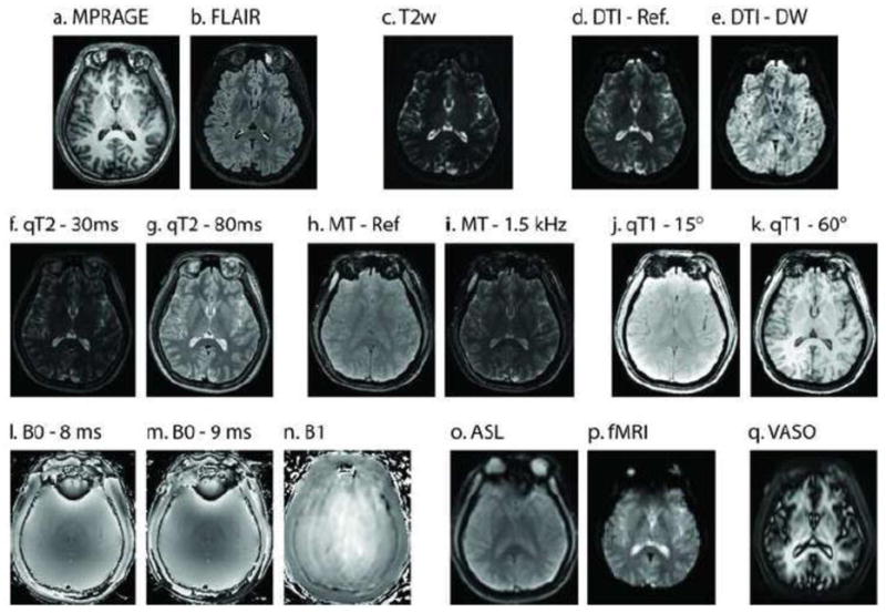
A single registered slice from the baseline images in the multi-parametric study of a representative subject. Structural scans (a–c) reveal high resolution information on local tissue classification. Diffusion (d–e), quantitative T2 (f–g), magnetization transfer (h–i), and quantitative T1 (j–k) provide assessments of local micro-structure. Field maps (l–n) enable improved calibration of quantitative findings. Assessment of perfusion (o–p) allows inference on functional characteristics.

Figure 2.

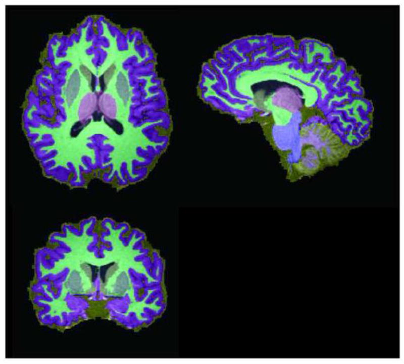
Representative whole brain segmentation for a single subject. Topologically correct segmentation yields volumetric segmentation of cortical gray matter (purple), cerebral white matter (cyan), thalamus (pink), putamen (slate), caudate (yellow), cerebellar white matter (lavender), brainstem (blue), cerebellar gray matter (marigold), and ventricular CSF (black). Sulcal CSF and dura are labeled separately (tan).

Table 2.

Estimate Volume of Regions of Interest

Region	Volume (cm3)	Scan-Rescan Coefficient of Variation	Intra-class Correlation Coefficient (ICC)*
	μ ± σ
Cortical GM	544.4±49.1	2.6%	0.959
Cerebral WM	442.6±45.4	1.5%	0.990
Ventricular CSF	17.2±9.4	4.0%	0.999
Thalamus	19.5±1.4	2.8%	0.912
Putamen	11.8±1.2	3.0%	0.961
Caudate	9.4±1.2	4.0%	0.951
Cerebellar GM	94.9±14.9	4.7%	0.955
Cerebellar WM	30.9±5.0	4.3%	0.961
Brainstem	21.9±2.7	4.7%	0.932
Cranial Vault and Posterior Fossa‡	1455.1±124.0	2.0%	0.978

Mean volumes are reported for all subjects. Standard deviation is reported across subjects. Scan-rescan C.V. is reported relative to the mean of the per-subject scan-rescan reproducibility.

^*All ICC’s significantly different from zero at the p<0.001 level.

^‡The volume of the cranial vault and posterior fossa is computed as the union of all non-skull structures (identified by SPECTRE).

Figure 3.

Illustrative contrasts derived from multi-parametric imaging. Anatomical information, such as tissue classification, cortical parcellation, local tissue diffusion characteristics, and white matter connectivity (a–d) can be inferred from structural and diffusion imaging. Voxel-wise MR properties, such as T1, T2, or MT ratio (e–g), can be inferred from quantitative imaging. Perfusion imaging reveals blood flow characteristics (e.g., perfusion, vascular density, or functional activity, h–j). Resting state fMRI data show the default mode network extracted using precuneus seed (green, MNI coordinates: −2 −51 27) correlation. B0 and B1 field mapping techniques (k–l) can be used to correct quantitative results and/or spatial distortions.

Observed image intensities are reported by the MRI scanner in arbitrary units that depend on numerous factors including amplifier gain, multi-channel fusion, conversion to 12- or 16-bit representations, etc. To compensate for this nuisance variability and ensure consistent reporting across modality, Table 3 reports the mean signal intensities normalized by the mean intensity of cerebral gray matter for each subject. Table 4 assesses the intra-region homogeneity for each imaging modality as defined as the standard deviation of the voxels within a region divided by the mean intensity of the corresponding region (i.e., the intra-region coefficient of variation). Table 5 summarizes scan-rescan reproducibility measures as the coefficient of variation across repetition, i.e., the standard deviation of the difference of repeated images within a region divided by the mean signal intensity in the region. The scan-rescan reproducibility can be interpreted as the noise-to-signal ratio (i.e., the inverse of the signal-to-noise, SNR); however, this metric is also sensitive to artifacts (systematic variation) and random variation between the scan-rescan events (Landman et al., 2009). Table 6 summarizes scan-rescan reproducibility measures in terms of ICC. Intra-session scan-rescan SNR is reported in Table 7.

Table 3.

Observed Signal: Mean Intensity by Region of Interest

Scan	Cortical GM	Cerebral WM	Ventricular CSF	Thalamus	Putamen	Caudate	Cerebellar GM	Cerebellar WM	Brainstem
	μ ± σ	μ ± σ	μ ± σ	μ ± σ	μ ± σ	μ ± σ	μ ± σ	μ ± σ	μ ± σ
FLAIR	1.05 ± 0.01	0.95 ± 0.06	0.47 ± 0.24	0.93 ± 0.04	0.92 ± 0.06	1.06 ± 0.05	1.11 ± 0.05	1.05 ± 0.08	1.04 ± 0.05
MPRAGE (Fast ADNI)	1.02 ± 0.02	1.78 ± 0.14	0.50 ± 0.28	1.82 ± 0.08	1.67 ± 0.06	1.52 ± 0.06	1.09 ± 0.06	1.83 ± 0.16	2.00 ± 0.17
DTI: Reference Image	1.06 ± 0.02	0.76 ± 0.06	2.66 ± 0.25	0.84 ± 0.06	0.76 ± 0.07	0.89 ± 0.10	1.04 ± 0.18	0.83 ± 0.12	0.90 ± 0.13
DTI: Diffusion Weighted	0.53 ± 0.03	0.43 ± 0.03	0.34 ± 0.05	0.44 ± 0.03	0.45 ± 0.04	0.50 ± 0.03	0.58 ± 0.10	0.48 ± 0.07	0.45 ± 0.07
DTI Geometric Reference	1.02 ± 0.02	0.69 ± 0.08	3.77 ± 0.62	1.08 ± 0.09	0.81 ± 0.09	1.09 ± 0.15	0.99 ± 0.07	0.77 ± 0.13	1.00 ± 0.16
Resting State fMRI	1.03 ± 0.04	0.95 ± 0.03	1.93 ± 0.24	1.17 ± 0.05	1.04 ± 0.06	1.16 ± 0.07	1.08 ± 0.12	1.09 ± 0.11	0.99 ± 0.15
B0 Magnitude (TE=8ms)	1.11 ± 0.07	1.07 ± 0.07	1.16 ± 0.20	1.47 ± 0.27	1.33 ± 0.27	0.84 ± 0.44	1.48 ± 0.75	1.60 ± 0.64	1.62 ± 0.65
B0 Magnitude (TE=9ms)	1.11 ± 0.07	1.07 ± 0.08	1.16 ± 0.19	1.47 ± 0.27	1.31 ± 0.27	0.82 ± 0.45	1.50 ± 0.74	1.62 ± 0.64	1.63 ± 0.66
B1 Magnitude	0.99 ± 0.05	1.08 ± 0.08	0.97 ± 0.23	0.97 ± 0.15	1.08 ± 0.46	0.86 ± 0.31	1.13 ± 0.10	1.10 ± 0.13	0.93 ± 0.12
Arterial Spin Labeling (ASL)	1.10 ± 0.06	0.97 ± 0.08	1.02 ± 0.22	1.19 ± 0.25	0.94 ± 0.35	0.66 ± 0.25	1.67 ± 0.73	1.61 ± 0.65	1.48 ± 0.57
VASO	1.14 ± 0.08	1.16 ± 0.21	1.45 ± 0.40	1.91 ± 0.49	1.40 ± 0.47	0.99 ± 0.40	2.01 ± 1.35	2.42 ± 1.24	2.12 ± 1.14
qT1 (15°)	1.00 ± 0.01	0.90 ± 0.02	0.78 ± 0.04	0.81 ± 0.02	0.86 ± 0.03	0.87 ± 0.02	0.92 ± 0.12	0.82 ± 0.05	0.76 ± 0.04
qT1 (60°)	1.00 ± 0.01	1.23 ± 0.02	0.68 ± 0.13	1.04 ± 0.04	1.12 ± 0.05	1.02 ± 0.04	1.06 ± 0.10	1.19 ± 0.07	1.11 ± 0.07
qT2 (dual echo: 30 ms)	1.09 ± 0.08	1.06 ± 0.07	1.29 ± 0.20	1.44 ± 0.27	1.31 ± 0.33	1.09 ± 0.35	1.29 ± 0.48	1.40 ± 0.54	1.52 ± 0.46
qT2 (dual echo: 80 ms)	0.65 ± 0.05	0.62 ± 0.05	0.80 ± 0.14	0.90 ± 0.19	0.74 ± 0.23	0.64 ± 0.21	0.78 ± 0.26	0.87 ± 0.36	0.97 ± 0.31
MT: Reference	1.09 ± 0.07	0.98 ± 0.05	1.00 ± 0.17	1.21 ± 0.24	1.18 ± 0.34	0.75 ± 0.37	1.35 ± 0.53	1.35 ± 0.44	1.31 ± 0.39
MT: 1.5 kHz	0.62 ± 0.05	0.54 ± 0.03	0.59 ± 0.11	0.70 ± 0.19	0.63 ± 0.21	0.43 ± 0.21	0.75 ± 0.24	0.74 ± 0.24	0.74 ± 0.19

Note σ is the standard deviation of mean intensities across subjects.

Table 4.

Intra-Region Homogeneity: Coefficient of Variation by Region of Interest

Scan	Cortical GM	Cerebral WM	Ventricular CSF	Thalamus	Putamen	Caudate	Cerebellar GM	Cerebellar WM	Brainstem
	μ ± σ	μ ± σ	μ ± σ	μ ± σ	μ ± σ	μ ± σ	μ ± σ	μ ± σ	μ ± σ
FLAIR	26% ± 5	16% ± 3	40% ± 8	21% ± 4	14% ± 3	23% ± 7	24% ± 6	19% ± 3	22% ± 5
MPRAGE (Fast ADNI)	34% ± 7	34% ± 8	37% ± 19	32% ± 5	16% ± 4	24% ± 10	30% ± 5	27% ± 7	30% ± 15
DTI: Reference Image	33% ± 4	14% ± 4	48% ± 19	26% ± 8	10% ± 3	22% ± 12	34% ± 11	20% ± 9	39% ± 14
DTI: Diffusion Weighted	16% ± 2	9% ± 1	9% ± 3	9% ± 1	6% ± 2	7% ± 2	17% ± 6	12% ± 3	15% ± 4
DTI Geometric Reference	42% ± 8	23% ± 8	111% ± 35	50% ± 14	14% ± 4	60% ± 27	36% ± 10	30% ± 16	39% ± 22
Resting State fMRI	30% ± 6	12% ± 2	23% ± 9	21% ± 5	10% ± 4	14% ± 7	27% ± 7	14% ± 3	25% ± 11
B0 Magnitude (TE=8ms)	63% ± 30	61% ± 33	58% ± 35	44% ± 37	39% ± 35	38% ± 22	25% ± 11	22% ± 13	25% ± 9
B0 Magnitude (TE=9ms)	64% ± 30	62% ± 33	59% ± 36	45% ± 38	39% ± 33	37% ± 21	25% ± 11	22% ± 13	25% ± 9
B1 Magnitude	54% ± 17	59% ± 25	39% ± 17	27% ± 14	42% ± 48	41% ± 23	27% ± 14	25% ± 7	22% ± 6
Arterial Spin Labeling (ASL)	76% ± 36	74% ± 38	60% ± 37	44% ± 44	38% ± 30	38% ± 20	26% ± 9	15% ± 4	15% ± 6
VASO	98% ± 31	95% ± 29	98% ± 31	106% ± 44	44% ± 14	52% ± 20	101% ± 52	100% ± 50	101% ± 42
qT1 (15°)	20% ± 2	10% ± 1	5% ± 1	7% ± 1	4% ± 1	5% ± 1	22% ± 9	9% ± 5	14% ± 7
qT1 (60°)	21% ± 3	13% ± 2	24% ± 6	17% ± 4	7% ± 1	14% ± 6	30% ± 13	15% ± 10	24% ± 10
qT2 (dual echo: 30 ms)	61% ± 29	60% ± 30	54% ± 23	43% ± 24	43% ± 35	53% ± 24	35% ± 10	37% ± 17	38% ± 11
qT2 (dual echo: 80 ms)	45% ± 16	44% ± 15	49% ± 12	47% ± 16	33% ± 23	44% ± 11	36% ± 11	44% ± 24	46% ± 18
MT: Reference	65% ± 29	59% ± 32	47% ± 31	34% ± 32	42% ± 37	34% ± 21	27% ± 13	18% ± 12	17% ± 8
MT: 1.5 kHz	41% ± 16	37% ± 17	37% ± 15	34% ± 21	25% ± 20	25% ± 11	27% ± 8	25% ± 10	24% ± 6

Note σ is the standard deviation of mean intensities across subjects.

Table 5.

Scan-Rescan Reproducibility: Coefficient of Variation by Region of Interest

Scan	Cortical GM	Cerebral WM	Ventricular CSF	Thalamus	Putamen	Caudate	Cerebellar GM	Cerebellar WM	Brainstem
	C.V.	C.V.	C.V.	C.V.	C.V.	C.V.	C.V.	C.V.	C.V.
FLAIR	6%	3%	26%	5%	3%	8%	4%	2%	3%
MPRAGE (Fast ADNI)	3%	1%	11%	1%	1%	1%	4%	2%	1%
DTI: Reference Image	6%	3%	5%	5%	2%	6%	13%	12%	13%
DTI: Diffusion Weighted	5%	2%	7%	2%	2%	2%	13%	10%	8%
DTI Geometric Reference	7%	6%	7%	7%	3%	9%	7%	5%	6%
Resting State fMRI	6%	2%	5%	4%	2%	3%	8%	3%	6%
B0 Magnitude (TE=8ms)	11%	19%	22%	15%	30%	95%	7%	2%	2%
B0 Magnitude (TE=9ms)	10%	18%	22%	14%	28%	105%	7%	2%	1%
B1 Magnitude	10%	13%	6%	6%	9%	10%	2%	2%	2%
Arterial Spin Labeling (ASL)	14%	28%	67%	27%	95%	161%	6%	2%	2%
VASO	9%	20%	74%	36%	117%	305%	16%	12%	10%
qT1 (15°)	2%	1%	1%	2%	1%	2%	11%	9%	5%
qT1 (60°)	4%	2%	6%	3%	1%	4%	17%	14%	10%
qT2 (dual echo: 30 ms)	14%	22%	24%	18%	28%	72%	6%	5%	4%
qT2 (dual echo: 80 ms)	16%	23%	24%	20%	28%	73%	9%	11%	8%
MT: Reference	11%	17%	20%	14%	32%	99%	8%	3%	2%
MT: 1.5 kHz	13%	19%	23%	20%	33%	79%	9%	6%	5%

Table 6.

Scan-Rescan Reproducibility: Intra-class Correlation Coefficient (ICC) by Region of Interest

Scan	Cortical GM	Cerebral WM	Ventricular CSF	Thalamus	Putamen	Caudate	Cerebellar GM	Cerebellar WM	Brainstem
FLAIR	0.76±0.039	0.77±0.028	0.83±0.032	0.75±0.029	0.70±0.028	0.68±0.057	0.73±0.038	0.75±0.023	0.73±0.028
MPRAGE (Fast ADNI)	0.91±0.014	0.94±0.008	0.88±0.023	0.93±0.006	0.82±0.015	0.86±0.025	0.87±0.019	0.86±0.021	0.82±0.025
DTI: Reference Image	0.87±0.024	0.88±0.014	0.86±0.020	0.90±0.015	0.82±0.026	0.86±0.025	0.76±0.039	0.76±0.050	0.79±0.053
DTI: Diffusion Weighted	0.82±0.024	0.82±0.009	0.48±0.024	0.67±0.016	0.51±0.030	0.55±0.033	0.69±0.045	0.69±0.042	0.70±0.038
DTI Geometric Reference	0.89±0.014	0.87±0.015	0.92±0.014	0.94±0.008	0.80±0.021	0.91±0.019	0.87±0.020	0.84±0.023	0.84±0.019
Resting State fMRI	0.82±0.048	0.72±0.029	0.63±NaN	0.70±0.054	0.62±0.036	0.65±0.051	0.70±0.053	0.65±0.057	0.73±0.044
B0 Magnitude (TE=8ms)	0.83±0.026	0.79±0.035	0.83±0.031	0.73±0.051	0.72±0.056	0.75±0.055	0.85±0.029	0.82±0.029	0.78±0.026
B0 Magnitude (TE=9ms)	0.79±0.030	0.75±0.041	0.77±0.057	0.74±0.058	0.69±0.071	0.71±0.058	0.80±0.035	0.76±0.040	0.73±0.037
B1 Magnitude	0.48±0.050	0.46±0.061	0.32±0.070	0.33±0.073	0.18±0.061	0.21±0.072	0.63±0.076	0.54±0.070	0.53±0.073
Arterial Spin Labeling (ASL)	0.92±0.008	0.91±0.010	0.87±0.033	0.80±0.027	0.79±0.044	0.76±0.056	0.81±0.025	0.70±0.031	0.70±0.039
VASO	0.94±0.005	0.93±0.008	0.83±0.034	0.82±0.041	0.82±0.041	0.67±0.056	0.90±0.014	0.88±0.019	0.87±0.016
qT1 (15°)	0.87±0.014	0.89±0.013	0.77±0.024	0.85±0.020	0.61±0.050	0.66±0.053	0.74±0.053	0.74±0.051	0.67±0.072
qT1 (60°)	0.81±0.026	0.79±0.028	0.86±0.023	0.88±0.021	0.63±0.036	0.75±0.061	0.70±0.065	0.71±0.064	0.61±0.066
qT2 (dual echo: 30 ms)	0.92±0.012	0.89±0.014	0.91±0.020	0.86±0.038	0.87±0.029	0.89±0.028	0.87±0.029	0.91±0.027	0.92±0.018
qT2 (dual echo: 80 ms)	0.90±0.016	0.89±0.016	0.91±0.022	0.88±0.039	0.87±0.023	0.89±0.028	0.87±0.030	0.91±0.025	0.93±0.017
MT: Reference	0.93±0.007	0.92±0.008	0.88±0.022	0.77±0.040	0.76±0.037	0.80±0.035	0.83±0.031	0.79±0.036	0.79±0.031
MT: 1.5 kHz	0.90±0.011	0.89±0.013	0.91±0.017	0.86±0.030	0.78±0.024	0.82±0.034	0.82±0.033	0.86±0.028	0.89±0.018

Mean ICC shown ± standard error.

Table 7.

Intra-Session SNR Measures

Scan	Corpus Callosum	Peripheral WM	Globus Palidus
FLAIR	10.9	17.0	13.4
MPRAGE (Fast ADNI)	25.6	30.2	25.5
DTI: Reference Image	13.1	36.7	30.1
DTI: Diffusion Weighted	8.2	11.8	11.0
DTI Geometric Reference	5.2	15.2	16.7
Resting State fMRI	24.2	36.8	40.6
B0 Magnitude (TE=8ms)	13.9	60.6	65.1
B0 Magnitude (TE=9ms)	6.9	55.8	39.2
B1 Magnitude	66.4	80.7	69.1
Arterial Spin Labeling (ASL)	48.8	56.5	79.3
VASO	26.3	68.6	30.4
qT1 (15°)	25.2	48.0	52.4
qT1 (60°)	25.9	46.6	35.1
qT2 (dual echo: 30 ms)	24.3	51.9	49.8
qT2 (dual echo: 80 ms)	11.7	30.3	23.6
MT: Reference	25.9	44.4	38.3
MT: 1.5 kHz	26.2	42.2	29.5

Discussion

In typical reproducibility assessments, results are reported for specific contrasts or measures of interest. Here, we take a distinct approach in terms of quantifying the reproducibility of only the directly observed quantities. These characterizations can be particularly informative for SNR, CNR, or power calculations to assess the potential effects of changes in voxel size, slice thickness, number of signal averages, or other simple protocol manipulations. Normal anatomical variability (both temporal and inter-subject characteristics) can make rescan-rescan data complex to interpret. In this study, we focus on isolating variation associated with the acquisition calibration and positioning rather than the anatomical and functional characteristics themselves. Hence, these data could be informative as to the detectable effect sizes over longer time courses.

A primary goal of this study is to measure experimental variability owing to methodology rather than natural biological variability. While fully removing biological variability is impossible, the impact of biological variability on these data can be sufficiently minimized. Actual biological variability is attenuated by having volunteers rescanned within an hour of initial scanning, while detected biological variability is minimized by choosing sufficiently large regions of interest for analysis. The regions of interest used in this study reflect the macroscopic organization of the brain (minimum volume approximately 10 cm3.) which are insensitive to small biological differences that may occur between scan and rescan. The observed variability from the ROI primarily reflects (1) tissue intensity level relative to the noise level, (2) propensity of a region to artifacts, and (3) regional sensitivity to variations in partial-volume effects. These data are therefore intended to provide the background noise level of an experimental methodology that one needs to determine the power of that method in measuring true biological variability within a smaller ROI.

Reproducibility of structural scans was higher than that of images targeting physiologically quantities. In the cortical GM and WM, T1 weighted scans (qT1 and MPRAGE) exhibited the highest reproducibility (mean C.V.< 2.2%), while DTI, fMRI and FLAIR exhibited good reproducibility (mean C.V.~ 5%). MT and quantitative T2 exhibited mean cortical reproducibility of C.V. 17%. ASL was the least reproducible in the cortical GM and WM with a mean C.V. of 21%. Notably, the ASL intensity in white matter exhibited a C.V. of 28%. Note that ASL is a perfusion sensitized measurement and WM has very low perfusion relative to cortical GM (which had a C.V. of 14%). VASO reproducibility was also low with a C.V. of 15%. Increased variability for quantitative scans is to be expected both because of physiological variability as well as the increased sensitivity for artifacts.

Although the structural scans (MPRAGE and FLAIR) exhibited consistent reliability between the brain and cerebellum, reproducibility of the sequences was not uniformly consistent for all scan types. ASL was exceptionally stable for cerebellar and brainstem structures (C.V. of <3%) while quantitative T2, MT, and field mapping approaches were also improved compare with cerebral structure (C.V. reduced by >11%). Yet, the quantitative T1 exhibited much lower reproducibility (C.V. increased by <7%) for brainstem regions. For deep brain structures (thalamus, putamen, caudate), there was strong correlation (ρ=0.74) between acquired slice thickness and C.V. of these structure. For deep brain structures, T1 weighted studies had high average reproducibility (<3% C.V.) while the ASL C.V. neared unity (94%) and the mean C.V. with VASO was 1.53. MT and quantitative T2 also performed poorly in the caudate (80% C.V.). CSF exhibited relatively low reproducibility (>5% C.V.) for all scans except quantitative T1, in which it was consistently of moderate intensity (~70% that of GM). The impact variability can be appreciated from the increased variability on bordering structures, especially those in which CSF is bright. For example, the caudate was poorly reproduced in scans with T2 weighted contrasts. The increase variability of

Herein, we tabulate the reproducibility of image intensities for large-scale neurological structures. These reproducibility measures are, by construction, less than that which one would expect if smaller, more homogeneous, regions were carefully placed. Specifically, we have intentionally included the effects of scan-rescan variation in artifact, distortion, partial voluming, and non-rigid motion that might corrupt subsequent analysis. The regions of interest were chosen to be representative of the large-scale regions which (1) are of general interest to community and (2) are reproducible with fully automated methods. More detailed characterizations would be valuable to specific fields, such as inclusion of a cortical parcellation or more precise characterization of white matter. However, these approaches would introduce additional methodological dependence and would likely benefit from careful consideration of the specific problem domain. Use of this data for comparative evaluation of anatomical characterizations (and their associated MR-derived contrasts) would be an interesting area of future research. Alternatively, regions of interest could be placed as to avoid these potential confounds if these effects would not be interfere with the data interpretation. We note that the variability measures themselves (e.g., resting state fMRI and diffusion weighted MRI intensities) are not always of direct interest. Rather, the scan-rescan variability measured presented herein can be used to model (either empirically or in simulation) the variability of derived parameters of interest. These data have been made public so that study-specific local regions of interest may be readily compared to the summary measures presented.

A direct analysis of the reliability and reproducibility does not mitigate the information contained in the resulting images. For example ASL has the lowest reproducibility, but it is the sole method for studying cerebral perfusion in the absence of contrast injection, so it is invaluable, though maybe not as reproducible as an approach that measures large scale changes in tissue water. Without a doubt, SNR plays a clear role in the reproducibility specific, yet a precise assessment of SNR for each contrast would necessitate either additional data (i.e., scan-rescan information within a session or noise-only scans) or making assumptions as to the where one could isolate of signal regions with true homogenous signal or use parametric modeling assumptions. As presented, this multi-parametric protocol can serve as a baseline set of sequences to which new generations of acquisition techniques can be compared.

Given the rather limited sample size (n=21), it is difficult to control for age and gender effects, which are known to modulate both brain structure and function. This heterogeneity does not necessarily undermine the assessment of within subject variation (so long as variability is not particularly associated with healthy aging). Furthermore, for power analyses, a hypothesis on effect size is also required. Here, we leave it to the reader to estimate effect size for the analyses methods and contrasts relevant to their endeavors. If imaging variability is believed to be strongly associated with demographics for a particular condition, the data are fully available so that cohorts may be repartitioned into representative populations and appropriate estimates of imaging characteristics may be estimated. The protocol has been fully released so additional acquisitions on select target populations with equivalent sequences are also possible and may be compared with those that have been presented.

There are ample opportunities to use this dataset to assess of specific metrics (e.g., quantitative parameters) and/or multi-parametric mapping (e.g., functional connectivity measures on cortical surfaces labeled with diffusion inferred connectivity). In many cases, the numerous potential approaches to derive the same metric are available and it would be an interesting scientific effort to compare such methods. Furthermore, these best practice methods may vary by intended application and require substantial exposition to detail the precise variant of a method used during analysis. Although these analyses are fascinating avenues for continuing study, such efforts are beyond the scope of this work. The authors are actively pursuing characterization of several approaches; however, independent efforts by other groups are also encouraged.

Conclusion

All resources for this manuscript have been publicly shared through the resource website of the national resource for quantitative functional MRI (http://mri.kennedykrieger.org/databases.html) and the “multimodal” project on the NITRC portal (http://www.nitrc.org/projects/multimodal/). The community is encouraged to use this data for investigation of the topics relevant to their research. Investigators who accept the BIRN Repository Data License may access, redistribute, and publish the data without justification of intended use. Forums are provided for researchers who, at their discretion, may seek to coordinate or collaborate on investigations.

In conclusion, this effort provides the neuroimaging community with a data resource that may be used for development, optimization, and evaluation of algorithms that exploit the diversity of modern MRI modalities. The data may contribute to or serve as a priori information for study planning, effect size estimation or as normative reference data from volunteers. Alternatively, the data may be used within an education or tutorial setting and hence provide realistic examples of the data available within clinical research. By optimizing a collection of modern MRI sequences to mutually run in under an hour, we have created a baseline for planning and more specialized study design at 3T.

Research Highlights.

• Present and evaluate a 60 minute multi-parametric imaging protocol at 3T.

• Assess brain function, structural, micro-architecture, and quantitative parameters.

• Tabulate intensity, variability and reproducibility of MR contrasts.

• Provides a resource for study planning and algorithm optimization.

• Establishes a baseline for development multi-parametric imaging protocols.

References

- Akel JA, Rosenblitt M, Irarrazaval P. Off-resonance correction using an estimated linear time map. Magn Reson Imaging. 2002;20:189–198. doi: 10.1016/s0730-725x(02)00487-3. [DOI] [PubMed] [Google Scholar]
- Alsop DC. The sensitivity of low flip angle RARE imaging. Magn Reson Med. 1997;37:176–184. doi: 10.1002/mrm.1910370206. [DOI] [PubMed] [Google Scholar]
- Andersson JL, Skare S, Ashburner J. How to correct susceptibility distortions in spin-echo echo-planar images: application to diffusion tensor imaging. Neuroimage. 2003;20:870–888. doi: 10.1016/S1053-8119(03)00336-7. [DOI] [PubMed] [Google Scholar]
- Ashburner J, Friston KJ. Unified segmentation. Neuroimage. 2005;26:839–851. doi: 10.1016/j.neuroimage.2005.02.018. [DOI] [PubMed] [Google Scholar]
- Bakker CJ, de Leeuw H, Vincken KL, Vonken EJ, Hendrikse J. Phase gradient mapping as an aid in the analysis of object-induced and system-related phase perturbations in MRI. Phys Med Biol. 2008;53:N349–358. doi: 10.1088/0031-9155/53/18/N02. [DOI] [PubMed] [Google Scholar]
- Balteau E, Hutton C, Weiskopf N. Improved shimming for fMRI specifically optimizing the local BOLD sensitivity. Neuroimage. 49:327–336. doi: 10.1016/j.neuroimage.2009.08.010. [DOI] [PMC free article] [PubMed] [Google Scholar]
- Bankman IN. Handbook of Medical Image Processing and Analysis. 2, illustrated. Academic Press; 2008. [Google Scholar]
- Barker GJ. Diffusion-weighted imaging of the spinal cord and optic nerve. J Neurol Sci. 2001;186(Suppl 1):S45–49. doi: 10.1016/s0022-510x(01)00490-7. [DOI] [PubMed] [Google Scholar]
- Barkhof F, Scheltens P. Imaging of white matter lesions. Cerebrovasc Dis. 2002;13(Suppl 2):21–30. doi: 10.1159/000049146. [DOI] [PubMed] [Google Scholar]
- Basser PJ. Fiber-tractography via diffusion tensor MRI. Proceedings of International Society for Magnetic Resonance in Medicine; Sydney, Australia. 1998. [Google Scholar]
- Basser PJ, Jones DK. Diffusion-tensor MRI: theory, experimental design and data analysis - a technical review. NMR Biomed. 2002;15:456–467. doi: 10.1002/nbm.783. [DOI] [PubMed] [Google Scholar]
- Basser PJ, Mattiello J, LeBihan D. Estimation of the effective self-diffusion tensor from the NMR spin echo. J Magn Reson B. 1994a;103:247–254. doi: 10.1006/jmrb.1994.1037. [DOI] [PubMed] [Google Scholar]
- Basser PJ, Mattiello J, LeBihan D. MR diffusion tensor spectroscopy and imaging. Biophys J. 1994b;66:259–267. doi: 10.1016/S0006-3495(94)80775-1. [DOI] [PMC free article] [PubMed] [Google Scholar]
- Bazin PL, Pham DL. Topology-preserving tissue classification of magnetic resonance brain images. IEEE Trans Med Imaging. 2007;26:487–496. doi: 10.1109/TMI.2007.893283. [DOI] [PubMed] [Google Scholar]
- Beaulieu C. The basis of anisotropic water diffusion in the nervous system - a technical review. NMR Biomed. 2002;15:435–455. doi: 10.1002/nbm.782. [DOI] [PubMed] [Google Scholar]
- Behzadi Y, Restom K, Liau J, Liu TT. A component based noise correction method (CompCor) for BOLD and perfusion based fMRI. Neuroimage. 2007;37:90–101. doi: 10.1016/j.neuroimage.2007.04.042. [DOI] [PMC free article] [PubMed] [Google Scholar]
- Biswal B, Yetkin FZ, Haughton VM, Hyde JS. Functional connectivity in the motor cortex of resting human brain using echo-planar MRI. Magn Reson Med. 1995;34:537–541. doi: 10.1002/mrm.1910340409. [DOI] [PubMed] [Google Scholar]
- Boly M, Phillips C, Tshibanda L, Vanhaudenhuyse A, Schabus M, Dang-Vu TT, Moonen G, Hustinx R, Maquet P, Laureys S. Intrinsic brain activity in altered states of consciousness: how conscious is the default mode of brain function? Ann N Y Acad Sci. 2008;1129:119–129. doi: 10.1196/annals.1417.015. [DOI] [PMC free article] [PubMed] [Google Scholar]
- Bottomley P, Ouwerkerk R. The dual-angle method for fast, sensitive T1 measurement in vivo with low-angle adiabatic pulses. J Magn Reson B. 1994;104:159–167. [Google Scholar]
- Brodmann K. Beiträge zur histologischen Lokalisation der Großhirnrinde. J Psychol Neurol. 1907;10:231–234. [Google Scholar]
- Busse RF. Reduced RF power without blurring: correcting for modulation of refocusing flip angle in FSE sequences. Magn Reson Med. 2004;51:1031–1037. doi: 10.1002/mrm.20056. [DOI] [PubMed] [Google Scholar]
- Busse RF, Hariharan H, Vu A, Brittain JH. Fast spin echo sequences with very long echo trains: design of variable refocusing flip angle schedules and generation of clinical T2 contrast. Magn Reson Med. 2006;55:1030–1037. doi: 10.1002/mrm.20863. [DOI] [PubMed] [Google Scholar]
- Buxton RB. The diffusion sensitivity of fast steady-state free precession imaging. Magn Reson Med. 1993;29:235–243. doi: 10.1002/mrm.1910290212. [DOI] [PubMed] [Google Scholar]
- Calhoun VD, Adali T, Pearlson GD, Pekar JJ. A method for making group inferences from functional MRI data using independent component analysis. Hum Brain Mapp. 2001;14:140–151. doi: 10.1002/hbm.1048. [DOI] [PMC free article] [PubMed] [Google Scholar]
- Carass A, Wheeler MB, Cuzzocreo J, Bazin P-L, Bassett SS, Prince JL. A Joint Registration and Segmentation Approach to Skull Stripping. 4th IEEE International Symposium on Biomedical Imaging: From Nano to Macro; 2007. pp. 656–659. [Google Scholar]
- Chagla GH, Busse RF, Sydnor R, Rowley HA, Turski PA. Three-dimensional fluid attenuated inversion recovery imaging with isotropic resolution and nonselective adiabatic inversion provides improved three-dimensional visualization and cerebrospinal fluid suppression compared to two-dimensional flair at 3 tesla. Invest Radiol. 2008;43:547–551. doi: 10.1097/RLI.0b013e3181814d28. [DOI] [PMC free article] [PubMed] [Google Scholar]
- Chalela JA, Alsop DC, Gonzalez-Atavales JB, Maldjian JA, Kasner SE, Detre JA. Magnetic Resonance Perfusion Imaging in Acute Ischemic Stroke Using Continuous Arterial Spin Labeling. Stroke. 2000;31:680–687. doi: 10.1161/01.str.31.3.680. [DOI] [PubMed] [Google Scholar]
- Clark CA, Werring DJ. Diffusion tensor imaging in spinal cord: methods and applications - a review. NMR Biomed. 2002;15:578–586. doi: 10.1002/nbm.788. [DOI] [PubMed] [Google Scholar]
- Clark CP, Brown GG, Eyler LT, Drummond SPA, Braun DR, Tapert SF. Decreased Perfusion in Young Alcohol-Dependent Women as Compared With Age-Matched Controls. The American Journal of Drug and Alcohol Abuse. 2007;33:13–19. doi: 10.1080/00952990601082605. [DOI] [PMC free article] [PubMed] [Google Scholar]
- Clark CP, Brown GG, Frank L, Thomas L, Sutherland AN, Gillin JC. Improved anatomic delineation of the antidepressant response to partial sleep deprivation in medial frontal cortex using perfusion-weighted functional MRI. Psychiatry Research: Neuroimaging. 2006;146:213–222. doi: 10.1016/j.pscychresns.2005.12.008. [DOI] [PMC free article] [PubMed] [Google Scholar]
- Constable RT, Anderson AW, Zhong J, Gore JC. Factors influencing contrast in fast spin-echo MR imaging. Magn Reson Imaging. 1992;10:497–511. doi: 10.1016/0730-725x(92)90001-g. [DOI] [PubMed] [Google Scholar]
- Conturo TE, Lori NF, Cull TS, Akbudak E, Snyder AZ, Shimony JS, McKinstry RC, Burton H, Raichle ME. Tracking neuronal fiber pathways in the living human brain. Proc Natl Acad Sci U S A. 1999;96:10422–10427. doi: 10.1073/pnas.96.18.10422. [DOI] [PMC free article] [PubMed] [Google Scholar]
- Cordes D, Haughton VM, Arfanakis K, Carew JD, Turski PA, Moritz CH, Quigley MA, Meyerand ME. Frequencies contributing to functional connectivity in the cerebral cortex in “resting-state” data. AJNR Am J Neuroradiol. 2001;22:1326–1333. [PMC free article] [PubMed] [Google Scholar]
- Cusack R, Brett M, Osswald K. An evaluation of the use of magnetic field maps to undistort echo-planar images. Neuroimage. 2003;18:127–142. doi: 10.1006/nimg.2002.1281. [DOI] [PubMed] [Google Scholar]
- Derdeyn CP, Videen TO, Yundt KD, Fritsch SM, Carpenter DA, Grubb RL, Powers WJ. Variability of cerebral blood volume and oxygen extraction: stages of cerebral haemodynamic impairment revisited. Brain. 2002;125:595–607. doi: 10.1093/brain/awf047. [DOI] [PubMed] [Google Scholar]
- Detre JA, Leigh JS, Williams DS, Koretsky AP. Perfusion imaging. Magn Reson Med. 1992;23:37–45. doi: 10.1002/mrm.1910230106. [DOI] [PubMed] [Google Scholar]
- Donahue MJ, Blakeley JO, Zhou J, Pomper MG, Laterra J, van Zijl PC. Evaluation of human brain tumor heterogeneity using multiple T(1)-based MRI signal weighting approaches. Magn Reson Med. 2008;59:336–344. doi: 10.1002/mrm.21467. [DOI] [PMC free article] [PubMed] [Google Scholar]
- Donahue MJ, Blicher JU, Ostergaard L, Feinberg DA, Macintosh BJ, Miller KL, Gunther M, Jezzard P. Cerebral blood flow, blood volume, and oxygen metabolism dynamics in human visual and motor cortex as measured by whole-brain multi-modal magnetic resonance imaging. J Cereb Blood Flow Metab. 2009a;29:1856–1866. doi: 10.1038/jcbfm.2009.107. [DOI] [PubMed] [Google Scholar]
- Donahue MJ, Hua J, Pekar JJ, van Zijl PC. Effect of inflow of fresh blood on vascular-space-occupancy (VASO) contrast. Magn Reson Med. 2009b;61:473. doi: 10.1002/mrm.21804. [DOI] [PMC free article] [PubMed] [Google Scholar]
- Donahue MJ, Lu H, Jones CK, Edden RA, Pekar JJ, van Zijl PC. Theoretical and experimental investigation of the VASO contrast mechanism. Magn Reson Med. 2006;56:1261. doi: 10.1002/mrm.21072. [DOI] [PubMed] [Google Scholar]
- Donahue MJ, van Laar PJ, van Zijl PC, Stevens RD, Hendrikse J. Vascular space occupancy (VASO) cerebral blood volume-weighted MRI identifies hemodynamic impairment in patients with carotid artery disease. J Magn Reson Imaging. 2009c;29:718. doi: 10.1002/jmri.21667. [DOI] [PMC free article] [PubMed] [Google Scholar]
- Edelman RR, Siewert B, Darby DG, Thangaraj V, Nobre AC, Mesulam MM, Warach S. Qualitative mapping of cerebral blood flow and functional localization with echo-planar MR imaging and signal targeting with alternating radio frequency. Radiology. 1994;192:513–520. doi: 10.1148/radiology.192.2.8029425. [DOI] [PubMed] [Google Scholar]
- Essig M, Waschkies M, Wenz F, Debus J, Hentrich HR, Knopp MV. Assessment of brain metastases with dynamic susceptibility-weighted contrast-enhanced MR imaging: initial results. Radiology. 2003;228:193–199. doi: 10.1148/radiol.2281020298. [DOI] [PubMed] [Google Scholar]
- Fatemi A, Smith SA, Dubey P, Zackowski KM, Bastian AJ, van Zijl PC, Moser HW, Raymond GV, Golay X. Magnetization transfer MRI demonstrates spinal cord abnormalities in adrenomyeloneuropathy. Neurology. 2005;64:1739–1745. doi: 10.1212/01.WNL.0000164458.02141.06. [DOI] [PubMed] [Google Scholar]
- Fox MD, Snyder AZ, Vincent JL, Corbetta M, Van Essen DC, Raichle ME. The human brain is intrinsically organized into dynamic, anticorrelated functional networks. Proceedings of the National Academy of Sciences of the United States of America. 2005;102:9673–9678. doi: 10.1073/pnas.0504136102. [DOI] [PMC free article] [PubMed] [Google Scholar]
- Funai AK, Fessler JA, Yeo DT, Olafsson VT, Noll DC. Regularized field map estimation in MRI. IEEE Trans Med Imaging. 2008;27:1484–1494. doi: 10.1109/TMI.2008.923956. [DOI] [PMC free article] [PubMed] [Google Scholar]
- Geurts JJ, Blezer EL, Vrenken H, van der Toorn A, Castelijns JA, Polman CH, Pouwels PJ, Bo L, Barkhof F. Does high-field MR imaging improve cortical lesion detection in multiple sclerosis? J Neurol. 2008;255:183–191. doi: 10.1007/s00415-008-0620-5. [DOI] [PubMed] [Google Scholar]
- Gholipour A, Kehtarnavaz N, Gopinath K, Briggs R, Panahi I. Average field map image template for Echo-Planar image analysis. Conf Proc IEEE Eng Med Biol Soc. 2008;2008:94–97. doi: 10.1109/IEMBS.2008.4649099. [DOI] [PubMed] [Google Scholar]
- Glover GH, Li TQ, Ress D. Image-based method for retrospective correction of physiological motion effects in fMRI: RETROICOR. Magn Reson Med. 2000;44:162–167. doi: 10.1002/1522-2594(200007)44:1<162::aid-mrm23>3.0.co;2-e. [DOI] [PubMed] [Google Scholar]
- Golay X, Jiang H, van Zijl PC, Mori S. High-resolution isotropic 3D diffusion tensor imaging of the human brain. Magn Reson Med. 2002;47:837–843. doi: 10.1002/mrm.10143. [DOI] [PubMed] [Google Scholar]
- Greicius MD, Flores BH, Menon V, Glover GH, Solvason HB, Kenna H, Reiss AL, Schatzberg AF. Resting-state functional connectivity in major depression: abnormally increased contributions from subgenual cingulate cortex and thalamus. Biol Psychiatry. 2007;62:429–437. doi: 10.1016/j.biopsych.2006.09.020. [DOI] [PMC free article] [PubMed] [Google Scholar]
- Greicius MD, Kiviniemi V, Tervonen O, Vainionpaa V, Alahuhta S, Reiss AL, Menon V. Persistent default-mode network connectivity during light sedation. Hum Brain Mapp. 2008;29:839–847. doi: 10.1002/hbm.20537. [DOI] [PMC free article] [PubMed] [Google Scholar]
- Greicius MD, Krasnow B, Reiss AL, Menon V. Functional connectivity in the resting brain: A network analysis of the default mode hypothesis. Proceedings of the National Academy of Sciences of the United States of America. 2003;100:253–258. doi: 10.1073/pnas.0135058100. [DOI] [PMC free article] [PubMed] [Google Scholar]
- Haacke EM. Magnetic resonance imaging: physical principles and sequence design. J. Wiley & Sons; New York: 1999. [Google Scholar]
- Hajnal JV, Bryant DJ, Kasuboski L, Pattany PM, De Coene B, Lewis PD, Pennock JM, Oatridge A, Young IR, Bydder GM. Use of fluid attenuated inversion recovery (FLAIR) pulse sequences in MRI of the brain. J Comput Assist Tomogr. 1992;16:841–844. doi: 10.1097/00004728-199211000-00001. [DOI] [PubMed] [Google Scholar]
- Helms G, Finsterbusch J, Weiskopf N, Dechent P. Rapid radiofrequency field mapping in vivo using single-shot STEAM MRI. Magn Reson Med. 2008;60:739–743. doi: 10.1002/mrm.21676. [DOI] [PMC free article] [PubMed] [Google Scholar]
- Hendrikse J, Petersen ET, Cheze A, Chng SM, Venketasubramanian N, Golay X. Relation Between Cerebral Perfusion Territories and Location of Cerebral Infarcts. Stroke. 2009;40:1617–1622. doi: 10.1161/STROKEAHA.108.539866. [DOI] [PubMed] [Google Scholar]
- Henkelman RM, Stanisz GJ, Graham SJ. Magnetization transfer in MRI: a review. NMR Biomed. 2001;14:57–64. doi: 10.1002/nbm.683. [DOI] [PubMed] [Google Scholar]
- Hoeffner EG, Case I, Jain R, Gujar SK, Shah GV, Deveikis JP, Carlos RC, Thompson BG, Harrigan MR, Mukherji SK. Cerebral perfusion CT: technique and clinical applications. Radiology. 2004;231:632–644. doi: 10.1148/radiol.2313021488. [DOI] [PubMed] [Google Scholar]
- Hornak JP, Szumowski J, Bryant RG. Magnetic field mapping. Magn Reson Med. 1988;6:158–163. doi: 10.1002/mrm.1910060204. [DOI] [PubMed] [Google Scholar]
- Horsfield MA, Jones DK. Applications of diffusion-weighted and diffusion tensor MRI to white matter diseases - a review. NMR Biomed. 2002;15:570–577. doi: 10.1002/nbm.787. [DOI] [PubMed] [Google Scholar]
- Hua J, Donahue MJ, Zhao JM, Grgac K, Huang AJ, Zhou J, van Zijl PC. Magnetization transfer enhanced vascular-space-occupancy (MT-VASO) functional MRI. Magn Reson Med. 2009a;61:944. doi: 10.1002/mrm.21911. [DOI] [PMC free article] [PubMed] [Google Scholar]
- Hua J, Qin Q, Donahue MJ, Zhou J, Pekar J, van Zijl PCM. Functional MRI Using Arteriolar Cerebral Blood Volume Changes. Proc. 17th Annual Meeting ISMRM; Hawaii, USA. 2009b. p. 12. [Google Scholar]
- Hua J, Qin Q, Pekar J, van Zijl PCM. Measuring Absolute Arteriolar Cerebral Blood Volume (CBVa) in Human Brain Gray Matter (GM) without Contrast Agent. Proc. 17th Annual Meeting ISMRM; Hawaii, USA. 2009c. p. 5314. [Google Scholar]
- Insko EK, Bolinger L. Mapping of the Radiofrequency Field. Journal of Magnetic Resonance Series A. 1993;103:82–85. [Google Scholar]
- Jack CR, Jr, Bernstein MA, Fox NC, Thompson P, Alexander G, Harvey D, Borowski B, Britson PJ, JLW, Ward C, Dale AM, Felmlee JP, Gunter JL, Hill DL, Killiany R, Schuff N, Fox-Bosetti S, Lin C, Studholme C, DeCarli CS, Krueger G, Ward HA, Metzger GJ, Scott KT, Mallozzi R, Blezek D, Levy J, Debbins JP, Fleisher AS, Albert M, Green R, Bartzokis G, Glover G, Mugler J, Weiner MW. The Alzheimer’s Disease Neuroimaging Initiative (ADNI): MRI methods. J Magn Reson Imaging. 2008;27:685–691. doi: 10.1002/jmri.21049. [DOI] [PMC free article] [PubMed] [Google Scholar]
- Jin T, Kim SG. Improved cortical-layer specificity of vascular space occupancy fMRI with slab inversion relative to spin-echo BOLD at 9.4 T. Neuroimage. 2008;40:59–67. doi: 10.1016/j.neuroimage.2007.11.045. [DOI] [PMC free article] [PubMed] [Google Scholar]
- Jovicich J, Czanner S, Han X, Salat D, van der Kouwe A, Quinn B, Pacheco J, Albert M, Killiany R, Blacker D, Maguire P, Rosas D, Makris N, Gollub R, Dale A, Dickerson BC, Fischl B. MRI-derived measurements of human subcortical, ventricular and intracranial brain volumes: Reliability effects of scan sessions, acquisition sequences, data analyses, scanner upgrade, scanner vendors and field strengths. Neuroimage. 2009;46:177–192. doi: 10.1016/j.neuroimage.2009.02.010. [DOI] [PMC free article] [PubMed] [Google Scholar]
- Kastrup O, Wanke I, Maschke M. Neuroimaging of infections. NeuroRx. 2005;2:324–332. doi: 10.1602/neurorx.2.2.324. [DOI] [PMC free article] [PubMed] [Google Scholar]
- Kelly AMC, Uddin LQ, Biswal BB, Castellanos FX, Milham MP. Competition between functional brain networks mediates behavioral variability. Neuroimage. 2008;39:527–537. doi: 10.1016/j.neuroimage.2007.08.008. [DOI] [PubMed] [Google Scholar]
- Koch KM, Papademetris X, Rothman DL, de Graaf RA. Rapid calculations of susceptibility-induced magnetostatic field perturbations for in vivo magnetic resonance. Phys Med Biol. 2006;51:6381–6402. doi: 10.1088/0031-9155/51/24/007. [DOI] [PubMed] [Google Scholar]
- Kochunov P, Duff Davis M. Development of structural MR brain imaging protocols to study genetics and maturation. Methods. 2009 doi: 10.1016/j.ymeth.2009.08.002. [DOI] [PMC free article] [PubMed] [Google Scholar]
- Kuppusamy K, Lin W, Cizek GR, Haacke EM. In vivo regional cerebral blood volume: quantitative assessment with 3D T1-weighted pre- and postcontrast MR imaging. Radiology. 1996;201:106–112. doi: 10.1148/radiology.201.1.8816529. [DOI] [PubMed] [Google Scholar]
- Landman BA, Bazin PL, Smith SA, Prince JL. Robust Estimation of Spatially Variable Noise Fields. Magn Reson Med. 2009;62:500–509. doi: 10.1002/mrm.22013. [DOI] [PMC free article] [PubMed] [Google Scholar]
- Larson-Prior LJ, Zempel JM, Nolan TS, Prior FW, Snyder AZ, Raichle ME. Cortical network functional connectivity in the descent to sleep. Proc Natl Acad Sci U S A. 2009;106:4489–4494. doi: 10.1073/pnas.0900924106. [DOI] [PMC free article] [PubMed] [Google Scholar]
- Le Bihan D. Molecular diffusion, tissue microdynamics and microstructure. NMR Biomed. 1995;8:375–386. doi: 10.1002/nbm.1940080711. [DOI] [PubMed] [Google Scholar]
- Le Bihan D, van Zijl P. From the diffusion coefficient to the diffusion tensor. NMR Biomed. 2002;15:431–434. doi: 10.1002/nbm.798. [DOI] [PubMed] [Google Scholar]
- Lee MA, Smith S, Palace J, Matthews PM. Defining multiple sclerosis disease activity using MRI T2-weighted difference imaging. Brain. 1998;121 (Pt 11):2095–2102. doi: 10.1093/brain/121.11.2095. [DOI] [PubMed] [Google Scholar]
- Lim KO, Helpern JA. Neuropsychiatric applications of DTI - a review. NMR Biomed. 2002;15:587–593. doi: 10.1002/nbm.789. [DOI] [PubMed] [Google Scholar]
- Lu H, Clingman C, Golay X, van Zijl PC. Determining the longitudinal relaxation time (T1) of blood at 3.0 Tesla. Magn Reson Med. 2004;52:679. doi: 10.1002/mrm.20178. [DOI] [PubMed] [Google Scholar]
- Lu H, Golay X, Pekar JJ, van Zijl PC. Functional magnetic resonance imaging based on changes in vascular space occupancy. Magn Reson Med. 2003;50:263. doi: 10.1002/mrm.10519. [DOI] [PubMed] [Google Scholar]
- Lu H, Law M, Johnson G, Ge Y, van Zijl PC, Helpern JA. Novel approach to the measurement of absolute cerebral blood volume using vascular-space-occupancy magnetic resonance imaging. Magn Reson Med. 2005a;54:1403. doi: 10.1002/mrm.20705. [DOI] [PubMed] [Google Scholar]
- Lu H, Nagae-Poetscher LM, Golay X, Lin D, Pomper M, van Zijl PC. Routine clinical brain MRI sequences for use at 3.0 Tesla. J Magn Reson Imaging. 2005b;22:13–22. doi: 10.1002/jmri.20356. [DOI] [PubMed] [Google Scholar]
- Lu H, Pollack E, Young R, Babb JS, Johnson G, Zagzag D, Carson R, Jensen JH, Helpern JA, Law M. Predicting Grade of Cerebral Glioma Using Vascular-Space Occupancy MR Imaging. AJNR Am J Neuroradiol. 2008;29:373–378. doi: 10.3174/ajnr.A0794. [DOI] [PMC free article] [PubMed] [Google Scholar]
- Lucas BC, Bogovic JA, Carass A, Bazin PL, Prince JL, Pham D, Landman BA. The Java Image Science Toolkit (JIST) for Rapid Prototyping and Publishing of Neuroimaging Software. Neuroinformatics. 2010;8:5–17. doi: 10.1007/s12021-009-9061-2. [DOI] [PMC free article] [PubMed] [Google Scholar]
- Marcus D, Wang T, Parker J, Csernansky J, Morris J, Buckner R. Open Access Series of Imaging Studies (OASIS): cross-sectional MRI data in young, middle aged, nondemented, and demented older adults. Journal of Cognitive Neuroscience. 2007;19:1498–1507. doi: 10.1162/jocn.2007.19.9.1498. [DOI] [PubMed] [Google Scholar]
- Marcus DS, Fotenos AF, Csernansky JG, Morris JC, Buckner RL. Open Access Series of Imaging Studies: Longitudinal MRI Data in Nondemented and Demented Older Adults. J Cogn Neurosci. 2009 doi: 10.1162/jocn.2009.21407. [DOI] [PMC free article] [PubMed] [Google Scholar]
- McAuliffe M, Lalonde F, McGarry D, Gandler W, Csaky K, Trus B. Medical image processing, analysis and visualization in clinical research. Computer-Based Medical Systems; 2001; 14th IEEE Symposium; 2001. pp. 381–386. [Google Scholar]
- McGraw KO, Wong SP. Forming inferences about some intraclass correlation coefficients. Psychological Methods. 1996;1:30–46. [Google Scholar]
- McKeown MJ, Jung TP, Makeig S, Brown G, Kindermann SS, Lee TW, Sejnowski TJ. Spatially independent activity patterns in functional MRI data during the stroop color-naming task. Proc Natl Acad Sci U S A. 1998;95:803–810. doi: 10.1073/pnas.95.3.803. [DOI] [PMC free article] [PubMed] [Google Scholar]
- Miyabe M, Mori S, van Zijl PC, Kirsch JR, Eleff SM, Koehler RC, Traystman RJ. Correlation of the average water diffusion constant with cerebral blood flow and ischemic damage after transient middle cerebral artery occlusion in cats. J Cereb Blood Flow Metab. 1996;16:881–891. doi: 10.1097/00004647-199609000-00012. [DOI] [PubMed] [Google Scholar]
- Moraal B, Roosendaal SD, Pouwels PJ, Vrenken H, van Schijndel RA, Meier DS, Guttmann CR, Geurts JJ, Barkhof F. Multi-contrast, isotropic, single-slab 3D MR imaging in multiple sclerosis. Eur Radiol. 2008;18:2311–2320. doi: 10.1007/s00330-008-1009-7. [DOI] [PubMed] [Google Scholar]
- Mori S, Crain BJ, Chacko VP, van Zijl PC. Three-dimensional tracking of axonal projections in the brain by magnetic resonance imaging. Ann Neurol. 1999;45:265–269. doi: 10.1002/1531-8249(199902)45:2<265::aid-ana21>3.0.co;2-3. [DOI] [PubMed] [Google Scholar]
- Mori S, Crain BJ, van Zijl PCM. 3D brain fiber reconstruction from diffusion MRI. Proceedings of International Conference on Functional Mapping of the Human Brain; Montreal, Canada. 1998. [Google Scholar]
- Mori S, Kaufmann WE, Pearlson GD, Crain BJ, Stieltjes B, Solaiyappan M, van Zijl PC. In vivo visualization of human neural pathways by magnetic resonance imaging. Ann Neurol. 2000;47:412–414. [PubMed] [Google Scholar]
- Mori S, van Zijl PC. Fiber tracking: principles and strategies - a technical review. NMR Biomed. 2002;15:468–480. doi: 10.1002/nbm.781. [DOI] [PubMed] [Google Scholar]
- Moseley ME, Chew WM, White DL, Kucharczyk J, Litt L, Derugin N, Dupon J, Brasch RC, Norman D. Hypercarbia-induced changes in cerebral blood volume in the cat: a 1H MRI and intravascular contrast agent study. Magn Reson Med. 1992;23:21–30. doi: 10.1002/mrm.1910230104. [DOI] [PubMed] [Google Scholar]
- Moseley ME, Cohen Y, Kucharczyk J, Mintorovitch J, Asgari HS, Wendland MF, Tsuruda J, Norman D. Diffusion-weighted MR imaging of anisotropic water diffusion in cat central nervous system. Radiology. 1990a;176:439–445. doi: 10.1148/radiology.176.2.2367658. [DOI] [PubMed] [Google Scholar]
- Moseley ME, Cohen Y, Mintorovitch J, Chileuitt L, Shimizu H, Kucharczyk J, Wendland MF, Weinstein PR. Early detection of regional cerebral ischemia in cats: comparison of diffusion- and T2-weighted MRI and spectroscopy. Magn Reson Med. 1990b;14:330–346. doi: 10.1002/mrm.1910140218. [DOI] [PubMed] [Google Scholar]
- Mueller SG, Weiner MW, Thal LJ, Petersen RC, Jack C, Jagust W, Trojanowski JQ, Toga AW, Beckett L. The Alzheimer’s disease neuroimaging initiative. Neuroimaging Clin N Am. 2005;15:869–877. xi–xii. doi: 10.1016/j.nic.2005.09.008. [DOI] [PMC free article] [PubMed] [Google Scholar]
- Mugler JP, 3rd, Brookeman JR. Three-dimensional magnetization-prepared rapid gradient-echo imaging (3D MP RAGE) Magn Reson Med. 1990;15:152–157. doi: 10.1002/mrm.1910150117. [DOI] [PubMed] [Google Scholar]
- Murphy K, Birn RM, Handwerker DA, Jones TB, Bandettini PA. The impact of global signal regression on resting state correlations: are anti-correlated networks introduced? Neuroimage. 2009;44:893–905. doi: 10.1016/j.neuroimage.2008.09.036. [DOI] [PMC free article] [PubMed] [Google Scholar]
- Oguz KK, Golay X, Pizzini FB, Freer CA, Winrow N, Ichord R, Casella JF, van Zijl PC, Melhem ER. Sickle cell disease: continuous arterial spin-labeling perfusion MR imaging in children. Radiology. 2003;227:567–574. doi: 10.1148/radiol.2272020903. [DOI] [PubMed] [Google Scholar]
- Ostergaard L, Sorensen AG, Kwong KK, Weisskoff RM, Gyldensted C, Rosen BR. High resolution measurement of cerebral blood flow using intravascular tracer bolus passages. Part II: Experimental comparison and preliminary results. Magn Reson Med. 1996a;36:726–736. doi: 10.1002/mrm.1910360511. [DOI] [PubMed] [Google Scholar]
- Ostergaard L, Weisskoff RM, Chesler DA, Gyldensted C, Rosen BR. High resolution measurement of cerebral blood flow using intravascular tracer bolus passages. Part I: Mathematical approach and statistical analysis. Magn Reson Med. 1996b;36:715–725. doi: 10.1002/mrm.1910360510. [DOI] [PubMed] [Google Scholar]
- Pierpaoli C, Jezzard P, Basser PJ, Barnett A, Di Chiro G. Diffusion tensor MR imaging of the human brain. Radiology. 1996;201:637–648. doi: 10.1148/radiology.201.3.8939209. [DOI] [PubMed] [Google Scholar]
- Portnoy S, Stanisz GJ. Modeling pulsed magnetization transfer. Magn Reson Med. 2007;58:144–155. doi: 10.1002/mrm.21244. [DOI] [PubMed] [Google Scholar]
- Poser BA, Norris DG. 3D single-shot VASO using a Maxwell gradient compensated GRASE sequence. Magn Reson Med. 2009;62:255. doi: 10.1002/mrm.22000. [DOI] [PubMed] [Google Scholar]
- Pruessmann KP, Weiger M, Scheidegger MB, Boesiger P. SENSE: Sensitivity encoding for fast MRI. Magnetic Resonance in Medicine. 1999;42:952–962. [PubMed] [Google Scholar]
- Raichle ME, MacLeod AM, Snyder AZ, Powers WJ, Gusnard DA, Shulman GL. A default mode of brain function. Proc Natl Acad Sci U S A. 2001;98:676–682. doi: 10.1073/pnas.98.2.676. [DOI] [PMC free article] [PubMed] [Google Scholar]
- Rajan SS. MRI: a conceptual overview. Springer; 1998. 1998. [Google Scholar]
- Reber PJ, Wong EC, Buxton RB, Frank LR. Correction of off resonance-related distortion in echo-planar imaging using EPI-based field maps. Magn Reson Med. 1998;39:328–330. doi: 10.1002/mrm.1910390223. [DOI] [PubMed] [Google Scholar]
- Risterucci C, Jeanneau K, Schoppenthau S, Bielser T, Kunnecke B, von Kienlin M, Moreau JL. Functional magnetic resonance imaging reveals similar brain activity changes in two different animal models of schizophrenia. Psychopharmacology (Berl) 2005;180:724–734. doi: 10.1007/s00213-005-2204-8. [DOI] [PubMed] [Google Scholar]
- Rudolf S, Paul W. Imaging of the active B1 field in vivo. Magnetic Resonance in Medicine. 1996;35:246–251. doi: 10.1002/mrm.1910350217. [DOI] [PubMed] [Google Scholar]
- Rumboldt Z, Marotti M. Magnetization transfer, HASTE, and FLAIR imaging. Magn Reson Imaging Clin N Am. 2003;11:471–492. doi: 10.1016/s1064-9689(03)00058-8. [DOI] [PubMed] [Google Scholar]
- Samson RS, Wheeler-Kingshott CA, Symms MR, Tozer DJ, Tofts PS. A simple correction for B1 field errors in magnetization transfer ratio measurements. Magn Reson Imaging. 2006;24:255–263. doi: 10.1016/j.mri.2005.10.025. [DOI] [PubMed] [Google Scholar]
- Schmierer K, Scaravilli F, Altmann DR, Barker GJ, Miller DH. Magnetization transfer ratio and myelin in postmortem multiple sclerosis brain. Ann Neurol. 2004;56:407–415. doi: 10.1002/ana.20202. [DOI] [PubMed] [Google Scholar]
- Schneider E, Glover G. Rapid in vivo proton shimming. Magn Reson Med. 1991;18:335–347. doi: 10.1002/mrm.1910180208. [DOI] [PubMed] [Google Scholar]
- Schwarzbauer C, Syha J, Haase A. Quantification of regional blood volumes by rapid T1 mapping. Magn Reson Med. 1993;29:709–712. doi: 10.1002/mrm.1910290521. [DOI] [PubMed] [Google Scholar]
- Seeley WW, Crawford RK, Zhou J, Miller BL, Greicius MD. Neurodegenerative diseases target large-scale human brain networks. Neuron. 2009;62:42–52. doi: 10.1016/j.neuron.2009.03.024. [DOI] [PMC free article] [PubMed] [Google Scholar]
- Seeley WW, Menon V, Schatzberg AF, Keller J, Glover GH, Kenna H, Reiss AL, Greicius MD. Dissociable intrinsic connectivity networks for salience processing and executive control. J Neurosci. 2007;27:2349–2356. doi: 10.1523/JNEUROSCI.5587-06.2007. [DOI] [PMC free article] [PubMed] [Google Scholar]
- Shehzad Z, Kelly AM, Reiss PT, Gee DG, Gotimer K, Uddin LQ, Lee SH, Margulies DS, Roy AK, Biswal BB, Petkova E, Castellanos FX, Milham MP. The resting brain: unconstrained yet reliable. Cereb Cortex. 2009;19:2209–2229. doi: 10.1093/cercor/bhn256. [DOI] [PMC free article] [PubMed] [Google Scholar]
- Shmatukha AV, Harvey PR, Bakker CJ. Correction of proton resonance frequency shift temperature maps for magnetic field disturbances using fat signal. J Magn Reson Imaging. 2007;25:579–587. doi: 10.1002/jmri.20835. [DOI] [PubMed] [Google Scholar]
- Shrout PE, Fleiss JL. Intraclass Correlations: Uses in Assessing Rater Reliability. Psychological Bulletin. 1979;86:420–428. doi: 10.1037//0033-2909.86.2.420. [DOI] [PubMed] [Google Scholar]
- Sled JG, Pike GB. Quantitative interpretation of magnetization transfer in spoiled gradient echo MRI sequences. J Magn Reson. 2000;145:24–36. doi: 10.1006/jmre.2000.2059. [DOI] [PubMed] [Google Scholar]
- Sled JG, Pike GB. Quantitative imaging of magnetization transfer exchange and relaxation properties in vivo using MRI. Magn Reson Med. 2001;46:923–931. doi: 10.1002/mrm.1278. [DOI] [PubMed] [Google Scholar]
- Smith SA, Farrell JA, Jones CK, Reich DS, Calabresi PA, van Zijl PC. Pulsed magnetization transfer imaging with body coil transmission at 3 Tesla: feasibility and application. Magn Reson Med. 2006;56:866–875. doi: 10.1002/mrm.21035. [DOI] [PubMed] [Google Scholar]
- Smith SA, Golay X, Fatemi A, Jones CK, Raymond GV, Moser HW, van Zijl PC. Magnetization transfer weighted imaging in the upper cervical spinal cord using cerebrospinal fluid as intersubject normalization reference (MTCSF imaging) Magn Reson Med. 2005;54:201–206. doi: 10.1002/mrm.20553. [DOI] [PubMed] [Google Scholar]
- Smith SM, Fox PT, Miller KL, Glahn DC, Fox PM, Mackay CE, Filippini N, Watkins KE, Toro R, Laird AR, Beckmann CF. Correspondence of the brain’s functional architecture during activation and rest. Proc Natl Acad Sci U S A. 2009;106:13040–13045. doi: 10.1073/pnas.0905267106. [DOI] [PMC free article] [PubMed] [Google Scholar]
- Sotak CH. The role of diffusion tensor imaging in the evaluation of ischemic brain injury - a review. NMR Biomed. 2002;15:561–569. doi: 10.1002/nbm.786. [DOI] [PubMed] [Google Scholar]
- Sporns O, Tononi G, Kotter R. The human connectome: A structural description of the human brain. PLoS Comput Biol. 2005;1:e42. doi: 10.1371/journal.pcbi.0010042. [DOI] [PMC free article] [PubMed] [Google Scholar]
- Stanisz GJ, Odrobina EE, Pun J, Escaravage M, Graham SJ, Bronskill MJ, Henkelman RM. T1, T2 relaxation and magnetization transfer in tissue at 3T. Magn Reson Med. 2005;54:507–512. doi: 10.1002/mrm.20605. [DOI] [PubMed] [Google Scholar]
- Stollberger R, Wach P. Imaging of the active B1 field in vivo. Magn Reson Med. 1996;35:246–251. doi: 10.1002/mrm.1910350217. [DOI] [PubMed] [Google Scholar]
- Talairach J, Tournoux P. Co-planar stereotaxic atlas of the human brain. Thieme; New York, NY: 1988. [Google Scholar]
- Tyszka JM, Mamelak AN. Quantification of B0 homogeneity variation with head pitch by registered three-dimensional field mapping. J Magn Reson. 2002;159:213–218. doi: 10.1016/s1090-7807(02)00101-5. [DOI] [PubMed] [Google Scholar]
- Ulug AM, Beauchamp N, Jr, Bryan RN, van Zijl PC. Absolute quantitation of diffusion constants in human stroke. Stroke. 1997;28:483–490. doi: 10.1161/01.str.28.3.483. [DOI] [PubMed] [Google Scholar]
- Valette J, Guillermier M, Boumezbeur F, Poupon C, Amadon A, Hantraye P, Lebon V. B(0) homogeneity throughout the monkey brain is strongly improved in the sphinx position as compared to the supine position. J Magn Reson Imaging. 2006;23:408–412. doi: 10.1002/jmri.20511. [DOI] [PubMed] [Google Scholar]
- van Gelderen P, de Vleeschouwer MH, DesPres D, Pekar J, van Zijl PC, Moonen CT. Water diffusion and acute stroke. Magn Reson Med. 1994;31:154–163. doi: 10.1002/mrm.1910310209. [DOI] [PubMed] [Google Scholar]
- van Osch MJ, Teeuwisse WM, van Walderveen MA, Hendrikse J, Kies DA, van Buchem MA. Can arterial spin labeling detect white matter perfusion signal? Magn Reson Med. 2009;62:165–173. doi: 10.1002/mrm.22002. [DOI] [PubMed] [Google Scholar]
- van Zijl PCM, Davis D, Moonen CTW. Diffusion Spectroscopy in Living Systems. In: Gillies RJ, editor. NMR in Physiology and Biomedicine. Academic Press; 1994. pp. 185–198. [Google Scholar]
- Vincent GvdV, Elia F, David P, Christian HR, David EJL. Functional connectivity as revealed by spatial independent component analysis of fMRI measurements during rest. Human Brain Mapping. 2004;22:165–178. doi: 10.1002/hbm.20022. [DOI] [PMC free article] [PubMed] [Google Scholar]
- Vincent JL, Patel GH, Fox MD, Snyder AZ, Baker JT, Van Essen DC, Zempel JM, Snyder LH, Corbetta M, Raichle ME. Intrinsic functional architecture in the anaesthetized monkey brain. Nature. 2007;447:83–86. doi: 10.1038/nature05758. [DOI] [PubMed] [Google Scholar]
- Volz S, Hattingen E, Preibisch C, Gasser T, Deichmann R. Reduction of susceptibility-induced signal losses in multi-gradient-echo images: application to improved visualization of the subthalamic nucleus. Neuroimage. 2009;45:1135–1143. doi: 10.1016/j.neuroimage.2009.01.018. [DOI] [PubMed] [Google Scholar]
- Webb P, Macovski A. Rapid, fully automatic, arbitrary-volume in vivo shimming. Magn Reson Med. 1991;20:113–122. doi: 10.1002/mrm.1910200112. [DOI] [PubMed] [Google Scholar]
- Weiskopf N, Hutton C, Josephs O, Turner R, Deichmann R. Optimized EPI for fMRI studies of the orbitofrontal cortex: compensation of susceptibility-induced gradients in the readout direction. Magma. 2007;20:39–49. doi: 10.1007/s10334-006-0067-6. [DOI] [PMC free article] [PubMed] [Google Scholar]
- Williams DS, Detre JA, Leigh JS, Koretsky AP. Magnetic resonance imaging of perfusion using spin inversion of arterial water. Proc Natl Acad Sci U S A. 1992;89:212–216. doi: 10.1073/pnas.89.1.212. [DOI] [PMC free article] [PubMed] [Google Scholar]
- Windischberger C, Robinson S, Rauscher A, Barth M, Moser E. Robust field map generation using a triple-echo acquisition. J Magn Reson Imaging. 2004;20:730–734. doi: 10.1002/jmri.20158. [DOI] [PubMed] [Google Scholar]
- Wolff SD, Balaban RS. Magnetization transfer contrast (MTC) and tissue water proton relaxation in vivo. Magn Reson Med. 1989;10:135–144. doi: 10.1002/mrm.1910100113. [DOI] [PubMed] [Google Scholar]
- Wu WC, Fernandez-Seara M, Detre JA, Wehrli FW, Wang J. A theoretical and experimental investigation of the tagging efficiency of pseudocontinuous arterial spin labeling. Magn Reson Med. 2007;58:1020–1027. doi: 10.1002/mrm.21403. [DOI] [PubMed] [Google Scholar]
- Xu J, Sun SW, Naismith RT, Snyder AZ, Cross AH, Song SK. Assessing optic nerve pathology with diffusion MRI: from mouse to human. NMR Biomed. 2008;21:928–940. doi: 10.1002/nbm.1307. [DOI] [PMC free article] [PubMed] [Google Scholar]
- Xue R, van Zijl PC, Crain BJ, Solaiyappan M, Mori S. In vivo three-dimensional reconstruction of rat brain axonal projections by diffusion tensor imaging. Magn Reson Med. 1999;42:1123–1127. doi: 10.1002/(sici)1522-2594(199912)42:6<1123::aid-mrm17>3.0.co;2-h. [DOI] [PubMed] [Google Scholar]
- Yarnykh VL. Actual flip-angle imaging in the pulsed steady state: a method for rapid three-dimensional mapping of the transmitted radiofrequency field. Magn Reson Med. 2007;57:192–200. doi: 10.1002/mrm.21120. [DOI] [PubMed] [Google Scholar]
- Yarnykh VL, Yuan C. Cross-relaxation imaging reveals detailed anatomy of white matter fiber tracts in the human brain. Neuroimage. 2004;23:409–424. doi: 10.1016/j.neuroimage.2004.04.029. [DOI] [PubMed] [Google Scholar]
- Yeo DT, Chenevert TL, Fessler JA, Kim B. Zero and first-order phase shift correction for field map estimation with dual-echo GRE using bipolar gradients. Magn Reson Imaging. 2007;25:1263–1271. doi: 10.1016/j.mri.2007.02.001. [DOI] [PMC free article] [PubMed] [Google Scholar]
- Yeung HN, Aisen AM. Magnetization transfer contrast with periodic pulsed saturation. Radiology. 1992;183:209–214. doi: 10.1148/radiology.183.1.1549673. [DOI] [PubMed] [Google Scholar]
- Yoshida T, Sugiura M, Naganawa S, Teranishi M, Nakata S, Nakashima T. Three-dimensional fluid-attenuated inversion recovery magnetic resonance imaging findings and prognosis in sudden sensorineural hearing loss. Laryngoscope. 2008;118:1433–1437. doi: 10.1097/MLG.0b013e318172ef85. [DOI] [PubMed] [Google Scholar]