

Abstract
We use open active contours to quantify cytoskeletal structures imaged by fluorescence microscopy in two and three dimensions. We developed an interactive software tool for segmentation, tracking, and visualization of individual fibers. Open active contours are parametric curves that deform to minimize the sum of an external energy derived from the image and an internal bending and stretching energy. The external energy generates (i) forces that attract the contour toward the central bright line of a filament in the image, and (ii) forces that stretch the active contour toward the ends of bright ridges. Images of simulated semiflexible polymers with known bending and torsional rigidity are analyzed to validate the method. We apply our methods to quantify the conformations and dynamics of actin in two examples: actin filaments imaged by TIRF microscopy in vitro, and actin cables in fission yeast imaged by spinning disk confocal microscopy.
Keywords: actin, microtubules, segmentation, tracking, active contours
INTRODUCTION
The assembly of actin and tubulin proteins and their bacterial homologs into long filaments underlies important cellular processes such as cell motility, intracellular transport, and cell division [Dumont and Mitchison, 2009; Margolin, 2009; Pollard and Cooper, 2009]. Image analysis of fluorescently-labeled cytoskeletal filaments has provided insights into the function of the cytoskeleton. Examples of such studies include measurements of actin polymerization rates using TIRF microscopy (TIRFM) in vitro [Fujiwara et al., 2007; Kuhn and Pollard, 2005], shapes of microtubules and actin filaments [Kass et al., 1996; Danuser et al 2000; Janson and Dogterom, 2004; Brangwynne et al., 2007a,b, 2008; Bicek et al., 2007 2009], shapes of MreB bundles in E. coli [Ausmees et al., 2003; Chiu et al., 2008], spatial distribution of actin stress fibers [Hayakawa et al., 2007; Hotulainen and Lappalainen, 2006; Kumar et al., 2006], and network morphology and distribution of intermediate filaments [Helmke et al., 2001; Mickel et al., 2008; Luck et al., 2009].
Reliably extracting information on the shapes of linear elements that correspond to filaments or bundles involves two image analysis tasks: segmentation (i.e., extracting the centerline of filaments), and tracking (i.e., measuring motion and deformation over time). A large body of prior work has described algorithms that aid in detection of dynamic linear structures in images.
In two dimensions (2D), semiautomated methods have been used to track actin filament ends for measuring elongation rates [Kuhn and Pollard, 2005]. Automated methods exist for tracking the tips of microtubules [Altinok et al., 2006; Jiang et al., 2006; Saban et al., 2006; Hadjidemetriou et al., 2008]. In Hadjidemetriou et al., [2004], the body of a microtubule can be extracted and tracked over frames using tangential constraints. Li et al. [2009a,b] used open active contour models to extract filaments and proposed mechanisms for handling filament intersections.
Related methods have been developed to extract linear and tubular structures in 3D images. Some model-free techniques, such as mathematical morphology [Zana and Klein, 2001], matching filters [Hoover et al., 2000], region growth [Masutani et al., 1998], and minimum description length [Yuan et al., 2009] have been used with considerable success. Model-based approaches have broader applications since they are more robust to noise and can conveniently integrate prior knowledge; these include particle filters [Florin et al., 2005], minimal path [Cohen and Kimmel, 1997], level set [Law and Chung, 2009], and snake-based methods [Sarry and Boire, 2001; Yim et al., 2001].
Several groups have made software that implements segmentation of linear structures freely available. This includes the 3D FIRE (FIbeR Extraction) Matlab code [Stein et al., 2008], the NeuriteTracer [Pool et al., 2008] and NeuronJ [Meijering et al., 2004] ImageJ plugins, and more recently, V3D-Neuron [Peng et al., 2010]. Visualization software aids in simultaneous viewing of the raw image data superimposed on segmented structures [Matula et al., 2009; Peng et al., 2010].
In this work we present a new, open source, software tool that allows segmentation and tracking of filamentous structures in both two and three dimensions. This tool is based on the “Stretching open active contours” SOACs algorithm [Li et al., 2009a]. Active contours, or “snakes,” [Kass et al., 1987] are deformable parametric curves. When placed on an image, an active contour deforms “actively” to minimize its associated energy. The total energy consists of an internal energy that makes the active contour smooth by penalizing abrupt changes in direction, and an external energy that represents constraints from the image data. The external energy generates forces that attract the curve toward salient image features. Conventional active contours are closed contours. In this work, we use open curves instead, to segment and track cytoskeletal filaments. The internal energy term remains the same as that in the original work [Kass et al., 1987]. Observing the appearance of bright ridges at approximately the central line of each filament, we designed two external energy terms: (i) an intensity-based energy term that is the lowest along the central bright ridges of the image, thus generating forces that attract the open active contour toward the centerline of a filament, and (ii) a stretching energy term that exerts forces at the curve’s two ends and stretches the active contour toward the ends of the filament in the image. Thus, we called these new active contours SOACs.
The software tool is called JFilament (http://athena.physics.lehigh.edu/jfilament/) and it is an ImageJ (http://rsbweb.nih.gov/ij/) plug-in. JFilament allows simultaneous visualization of 2D, 3D or 4D (3D space + 1 time) images together with graphical curves representing segmented filaments. Users can deform, add, delete, save, and load filament curves. The overview flowchart of the JFilament is illustrated in Fig. 1A. The main page of the JFilament user interface is shown in Fig. 1B. In addition to SOACs, JFilament includes standard “closed” active contours which can be used for tasks such as segmentation and tracking of cell boundaries.
Fig. 1. (A) The flowchart of the JFilament program. (B) A snapshot of the graphical user interface.

In this article, we further show how JFilament can be used to quantify static and dynamics properties of cytoskeletal filaments, such as bending and torsional persistence lengths (lp and lτ, respectively), and elongation rates. First, to validate our analysis, we generated simulated images of filaments with known lp and lτ. JFilament was used successfully to measure these lengths. Then, we applied our methods to two cases involving images from experiments: (i) measurements of persistence length and elongation rate of actin filaments imaged by TIRFM in vitro, and (ii) measurements of bending and torsional properties of fluorescently labeled actin cables in fission yeast, imaged by confocal microscopy. We report the first measurements of configurational statistics of actin cables in 3D.
Methods
Data: Static and Time-Lapsed Images
JFilament was designed to be used primarily for analysis of single-color fluorescence microscopy images. Typically these are (i) stacks of 2D images with each frame representing different time (as with epifluorescence or TIRFM images), or (ii) 4D stacks, with each time point represented by a 3D stack. We assume that the 3D stacks consist of equidistant confocal microscopy planes or deconvoluted epifluorescence focal planes. We used JFilament to analyze images of in vitro actin polymerization obtained by TIRFM from Fujiwara et al. [2007] and confocal microscopy images of actin cables in fission yeast labeled by GFP-CHD from Vavylonis et al. [2008].
Filament Segmentation using SOACs
To locate the bright ridges that correspond to filaments, we used SOACs which are open active contours that minimize the sum of an internal and external energy [Kass et al., 1987; Li et al., 2009a]. The internal energy of SOACs favors shorter and straighter active contours. An image-based external energy term attracts them toward the bright ridges at the central lines of filaments and extends them along linear elements depending on the location of the end points.
In 2D, let r(s) = (x(s),y(s)), s ∈ [0,L] represent an open curve parametrically (Fig. 2), where s represents arc length along the open curve, and L is the length of the active contour. In 3D, r(s) = (x(s),y(s),z(s)), where s ∈ [0,L]. The starting and the ending points of the active contour are s = 0 and s = L respectively. A set of N sampling points ri = (xi,yi), i = 1, ⋯, N, (or in 3D ri = (xi,yi,zi), i = 1, ⋯, N), is sampled from the active contour to represent it. The points are sampled at approximately evenly spaced intervals.
Fig. 2. Illustration of the open active contour model, where s ∈ [0,L] measures contour length.
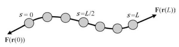
Points (dots) are uniformly sampled on the active contour. N is the total number of sampling points on the active contour. Internal energy favors snake shrinking and penalizes abrupt direction change along the active contour. Stretching forces (arrows) are applied at the tips (r(0) and r(L)) and point outward along the contour’s tangent directions. The forces are intensity-adaptive. If the tip of the active contour is on the filament body then the force points outward to stretch the active contour; if the tip is in the background, the force points inward to shrink the contour.
The active-contour-based segmentation works by minimizing the contour’s overall energy, E, which is composed of internal energy, Eint, and external energy, Eext, i.e.,
| (1) |
The internal energy term makes the active contour smooth by penalizing abrupt changes in direction. The external energy term represents forces from the image data.
Internal energy term
The internal energy term, Eint, is defined similar to closed snakes [Kass et al., 1987]:
| (2) |
where rs(s) ≡ dr/ds and rss(s) ≡ d2r/ds2. The first term, ∣rs(s)∣2, penalizes stretching; the second term, ∣rss(s)∣2, penalizes bending.
External snake energy
The external energy, Eext, consists of two terms: an image term, Eimg, and a stretching term, Estr:
| (3) |
where k is a constant that balances the internal and external energy contributions, and kstr is a constant that balances the two external energy terms, which are defined below.
We use a Gaussian-filtered image, Eimg = Gλ ∗ I, as the image term, where Gλ is the Gaussian smoothing kernel, I denotes the original image, and * denotes the 2D or 3D filtering operator [Gonzalez and Woods, 2007]. The degree of smoothing can be adjusted in JFilament by changing parameter λ. This term is different from the gradient magnitude term ∣∇Gλ * I∣2 commonly used in conventional segmentation methods [Kass et al., 1987 Xu and Prince, 1998]. As shown in Fig. 3, the gradient vectors corresponding to ∇Eimg point toward the center of filaments. Therefore, our image term has the desired property of attracting the active contour toward the central bright ridge of the filament.
Fig. 3. TIRFM image of a single actin filament and illustration of the gradient field of our image term, Eimg = Gλ * I.
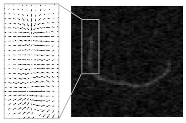
The gradient vectors point toward the center of the filament. Therefore, the image term attracts the active contour toward the central line of the filament.
The gradient vectors of the image term, ∇Eimg, cannot attract the tips of the active contour to grow along the filament body. In order to give an active contour the ability to stretch along a filament body, stretching forces are added to tips of the active contour (s = 0 and s = L). The tip stretching forces point outwards along the tangent direction of the active contour as shown in Fig. 2. The direction is −t(s) if s = 0 and t(s) if s = L, where . The magnitude of the stretching force is given by:
| (4) |
where I(r(s)) denotes the pixel intensity value covered by a certain point r(s) on the active contour, If denotes the mean foreground (i.e. filament) intensity, Ib denotes the mean background intensity, and Imean denotes the average intensity. Parameters, If,Ib,Imean, are constants and they are estimated using foreground and background training samples before segmentation. When the intensity at the snake tip is greater than Imean the force will stretch the snake. If the tip is located at a region of lower intensity than Imean, the force causes the active contour to shrink. Given the stretching force definition, we have the gradient field of the stretching energy term as:
| (5) |
Active contour deformation
An open active contour deforms and stretches under the influence of forces generated by the above internal and external energy terms. Similarly to Kass et al. [1987], the energy function of our new SOAC model is minimized using the Euler method. Since the active contour is represented by a set of discrete points, its overall energy E can be approximated by a sum of energies at these points:
| (6) |
where and denote the internal and external energy at the ith point of the active contour, respectively. The derivatives of and can be calculated with finite differences in 2D or 3D. Euler’s method is used to derive the dynamics of the active contour. Therefore we minimize the energy function (6) by iteratively solving for the coordinates of all points and following the model evolution equations:
| (7) |
| (8) |
in 2D, and,
| (9) |
| (10) |
| (11) |
in 3D. In the equations, A is a strictly penta-diagonal banded matrix created based on α and β (Eq. 2) and encodes the derivatives of internal energy for every point. I is the identity matrix, x, y, and z are the vectors representing the sets of x, y, and z coordinates, ξ is the step size in Euler’s method, and the subscript n denotes the iteration number.
Using the above optimization method, an open active contour can efficiently deform to desired filament central line locations. During its deformation, the active contour is resampled every few iterations, maintaining the distance between adjacent sampling points at a fixed interval Δssnake. Thus as the active contour grows longer, the number of sampling points increases, enabling the active contour to elongate. An example of the deformation process of our active contour model is shown in Fig. 4A. Note that although the initialization is far away from the actual filament location (Fig. 4A, i), the active contour is able to correctly recover the filament central ridges (Fig. 4A, iv). In JFilament, the user is able to pick the desired number of iterations that are sufficient to ensure convergence.
Fig. 4. Examples of segmentation and tracking of linear structures in 2D and 3D.

In (A)–(C) units are in pixels. A: Examples of segmentation of an actin filament in a TIRFM image. (i) Initialization of the active contour away from the central line of the filament. (ii)–(iv) The active contour after 20, 40, and 80 iterations of deformation. B: Images of actin filament polymerization over time using TIRFM. Panels (i)–(iv) correspond to frames 1, 4, 9 and 13. The growth occurs primarily at the barbed end. C: Illustration of tracking filament growth in panel B using SOACs. Red, green, cyan, and purple curves show SOACs for frames 1, 4, 9, and 13. Frame drift and filament shape changes can be observed; SOACs can adapt to these changes. D: Illustration of 3D views together with filament segmentation results. The images show a fission yeast cdc25-22 cell expressing GFP-CHD that marks actin cables and actin patches [Vavylonis et al., 2008]. (i) 3D volume view and active contour of a segmented actin cable. (ii) Image of an active contour together with x,y and z cross-sections of the image.
User interaction and manual editing
We have included manual controls that increase throughput and segmentation accuracy. In addition to initialization, the ends of active contours can also be trimmed or stretched and the middle of filaments can be cropped. These simple modifications enable more accurate results by allowing the user to solve the difficulties caused by intersections or variations in intensity that are hard to predict and automate. The user can define 3D points by clicking on cross-section planes.
Filament Tracking using SOACs
An active contour can be added and initialized manually at any time point k of a 2D or 3D image sequence. The converged snake of the kth time point is used to initialize the active contour for time point k + 1. Thus, the active contour can adapt by growing or shrinking, following the growth or shrinkage of the filament in the image over time. An example is shown in Fig. 4B and 4C where the red curve denotes the active contour computed based on a filament in the first frame. The green curve represents the active contour computed for the same filament in the fourth frame. Image sequences may often show drift, i.e. translation, between contiguous frames [Kuhn and Pollard, 2005]. Our algorithm is robust to mild frame drift and filament shape changes since the snake is allowed to re-equilibrate along the shifted images. An example of this is shown in Fig. 4C.
Visualization
Visualization and user interactions in 3D are more challenging than those in 2D. We used Java3D for simultaneous visualization of 3D images and segmentation results represented by active contours. Figure 4D shows an example. The active contour, representing the segmented filament is shown on top of a 3D volume view (panel 4D, i). Another window shows the position of the active contour with respect to cross sections of the image with the yz, zx, and xy planes; the three planes can be moved along the x, y, and z axes (panel 4D, ii). The visualization platform supports rendering of 4D images.
Curve properties
The parametric equation of a 3D snake curve, r(s), can be used to evaluate the set of three Frenet–Serret orthonormal vectors, namely the tangent (t), normal (n), and binormal (b) vectors at position s [Jose and Saletan, 1998], see Fig. 5:
| (12) |
| (13) |
| (14) |
Fig. 5. A cartoon showing a filament and sets of Frenet-Serret orthonormal vectors (tangent, t; normal, n; binormal b; see Eq. 14) at points i and j along the filament.
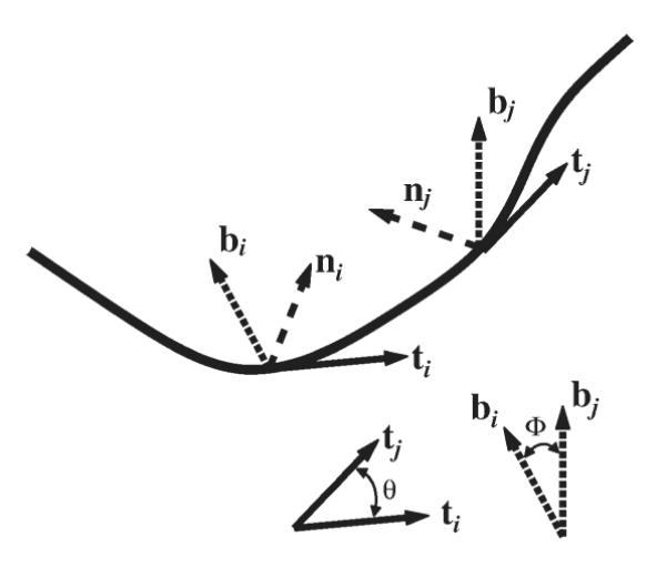
The vector drawings at the bottom right show the angle between tangent vectors and the angle between binormal vectors at points i and j, respectively. Averaging over such angles is used in the calculation of the tangent and binormal correlation functions.
The curvature, κ, and torsion, τ, are determined by the rates of change of the tangent vector and binormal vector with respect to the arc length:
| (15) |
Curvature represents the rate at which the curve deviates from a straight line on a plane. Torsion represents the rate at which the curve goes out of a plane. A 2D curve has zero torsion (constant binormal vector).
The shapes of snakes extracted from the image can be used to describe the statistical properties of an ensemble of curves that represent filaments or bundles. Such quantities include the probability distributions of curvature and torsion. Other statistical quantities are the tangent and binormal correlations. The tangent correlation function is defined as the ensemble average of the product of tangent vectors separated by a distance Δs:
| (16) |
Here, 〈〉 represents the average over all filaments and over all s along each filament. Similarly, the binormal correlation function is defined as the ensemble average of the product between binormal vectors separated by a distance Δs:
| (17) |
The tangent correlation function measures how fast a curve changes orientation while the binormal correlation function measures how fast the curve goes out of a plane.
Simulated Semiflexible Filaments
Filament model
For testing purposes, we constructed simulated images of equilibrium semiflexible polymers (worm-like chains, WLCs) in 2D and 3D described by the following Hamiltonian:
| (18) |
where b is the bending rigidity and bτ is the torsional rigidity. The last term representing torsion is absent in 2D. In 3D, this model represents a chain with uniform bending and torsional rigidity but no coupling between bending and torsion. In general, the energetics of biopolymers involve coupled bending, torsion and twist [Marko and Siggia, 1994]. Equation 18 does not include filament twist which is a property that is not captured by SOACs. Even though H is not the most general Hamiltonian to describe WLCs, it is useful as a model for validation since its equilibrium properties are known and easy to simulate.
In the model of Eq. 18, the tangent correlation function decays exponentially and is given by [Landau and Lifshitz, 1980]
| (19) |
where d is dimensionality and lp = b/kBT is the persistence length. Similarly, the binormal correlation function is given by [Giomi and Mahadevan, 2010]
| (20) |
where lτ = bτ/kBT is the torsional persistence length.
The curvature distribution P(κ), the probability density for observing a value of curvature between κ and κ + dκ, depends on the dimension [Rappaport et al., 2008]:
| (21) |
| (22) |
where Δsc is the length between sampling points along the curve that are used to calculate the curvature. In the model of Eq. 18 where there is no coupling between bending and torsion, the torsion is distributed as exp{−Htorsion/kBT}. Thus, the probability density for obtaining a value of torsion between τ and τ + dτ is
| (23) |
In addition to using correlation functions and curvature/torsion distributions, the properties of semiflexible filaments can also be studied by Fourier analysis. For a 2D curve, the amplitude of the nth Fourier mode is , where θ(s) is the tangent angle at position s. When a 2D curve representing an equilibrium semiflexible polymer is measured with mean square point localization error ε2, the mean square Fourier amplitudes satisfy [Gittes et al., 1993]:
| (24) |
where N is the number of sample points along the curve. The persistence length lp can be evaluated by fitting to Eq. 21.
Generation of images of filaments
Trajectories of 2D semiflexible filaments were generated using a walk of constant step size δ. An angle θ between the displacement vectors of successive steps was chosen from a Gaussian distribution centered at θ = 0 and variance σθ. The variance and the step size determine the persistence length of the filament. Expanding Eq. 16 and 19 for small θ and Δs, respectively, one has 1 −〈θ2〉/2 ≂ 1 −δ/2lp. Thus, the persistence length is [Rappaport et al., 2008]:
| (25) |
The statistics of the resulting angular distributions are identical to those of a 2D WLC down to the level of a single step of the walk. Images were generated by convoluting the trajectory of the walk with a Gaussian kernel.
Simulated images of filaments in 3D were generated similarly to 2D. The angle θ between successive displacement vectors was drawn from the distribution [Rappaport et al., 2008], with θ positive or negative. The torsional angle ϕ describing the rotation of the plane defined by two successive steps was chosen from a Gaussian distribution centered at ϕ = 0 with variance σϕ. Expanding Eq. 16 and 19, one has 1 −〈θ2〉/2 ≂ 1 −δ/lp. Using , we find:
| (26) |
The second of Eq. 26 follows similarly from Eq. (17) and (20). The generated trajectories obey the statistics of Eq. 18 down to a single step of the walk. Images were generated by convoluting the trajectory of the walk with a Gaussian which is 3 times wider along the direction in between z-slices, mimicking an experimental point spread function (PSF) of a confocal microscope.
Results
In this section we demonstrate how JFilament can be used to quantify static and dynamics properties of cytoskeletal filaments. We start by validating our analysis using simulated images of semiflexible polymers of known properties.
Validation using Simulated 2D Semiflexible Polymers
We generated simulated images of 2D WLCs using walks of step size δ = 1/20 pixel and total length 170 pixels, as described in the Methods section. The persistence length of these chains was varied by changing the parameter σθ, see Eq.25. Theresulting trajectories were convoluted with a 2D Gaussian of variance 1 pixel to generate images such as those in Fig. 6A.
Fig. 6. Analysis on 2D simulated filaments with known persistence lengths (lp = 500, 222, and 125 pixels) and total length L = 170 pixels.

The coarse-graining length is Δsc =Δssnake = 1 pixel and 40 filaments were used. A: Typical image with lp = 125 pixels. B: Plot of tangent correlations and fits to a single exponential. Error bars indicate standard deviation of individual measurements. = The values of the extracted persistence length are shown on the panel. These values are close to the intrinsic persistence lengths of the WLCs. C: Plot of curvature distribution and Gaussian fits (cf. Eq. 21). The measured persistence lengths shown on the plot are much longer than the intrinsic persistence length of the WLCs (see main text for discussion). D: Plots of mean square amplitude of Fourier modes versus mode number for intrinsic persistence length 500, 222, and 125 in panels (i)–(iii), respectively. Continuous lines are fits to Eq. 24; the corresponding values of lp and ε are shown in the panels. The dashed line in panel (i) shows the results of Eq. 24 using lp = 500 and ε = 0.14 (see main text).
We used JFilament to generate active contours that adapted to the bright ridges of the simulated image. The distance between successive points on the snake was set to Δssnake = 1 pixel. The other parameters of the snakes (such as α, β and γ, see Methods section) were adjusted manually until good agreement was achieved by visual inspection. The parametric curves of the snakes were then used to calculate the tangent correlation function, curvature distribution and amplitudes of Fourier modes (see Figs. 6B, 6C, and 6D).
Figure 6B shows the tangent correlation function for three different values of the WLC persistence length. After fitting to single exponentials, see Eq. 19, we were able to obtain estimates of the persistence length that were within 10% of the value of the intrinsic persistence length of the WLCs. Fits to Fourier amplitudes in Fig. 6D, using Eq. 24, give similar estimates for the persistence length, see Table I.
Table I.
Table Showing Agreement Between Intrinsic and Measured Persistence Length of Simulated 2D Worm-Like Chains (units: pixels)
| lp (WLC) | lp (tangent correlation) | lp (Fourier) | |
|---|---|---|---|
| σθ = 0.01 | 500 | 540 | 525 |
| σθ = 0.015 | 220 | 240 | 253 |
| σθ = 0.02 | 125 | 140 | 110 |
The intrinsic persistence length was varied by changing parameter σθ. The measured persistence length was extracted from fits to the tangent correlation function and mean square Fourier amplitudes in Fig. 6.
We found that the curvature distribution can also provide a good estimate of the persistence length, but this requires caution, as discussed in Bicek et al. [2007]. Figure 6C shows the curvature distribution for the same snakes as those used in Figs. 6B, and 6D. In this panel, a value for the curvature was calculated from each triplet of successive points of the snake; on average, the successive points were separated by distance Δsc = Δssnake. The resulting curvature distributions follow Gaussian profiles, as expected from Eq. 21. However, fitting these curves to Eq. 21 results in a predicted persistence length which is an order of magnitude higher than the intrinsic persistence length of the WLC.
The problem with the values obtained in Fig. 6B is that they reflect the bending stiffness of the active contour, in addition to that of the WLC. Because of our choice of snake parameters, locally, i.e. on scales of order a pixel, the snake appears stiffer than the WLC. This behavior is also evident in downward trend of in Fig. 6D at mode numbers n ~ 30: the data deviate from the expected scaling of slope −2 and lie below the fit of Equation 24. This deviation indicates a stiffening of the snake on short scales. Consistently, the slope of the tangent correlation function at s = 1 pixel in Fig. 6B is somewhat smaller than the slope at s = 20, implying larger persistence length at small distances. However, since the relative decay of the tangent correlation over small distances is small, the exponential fit is dominated by the decay of the tangent correlation over distances much longer than a pixel; thus the correct persistence length is recovered by the exponential fit.
It is useful to compare the results of Fig. 6D to the method of Brangwynne et al. [2007a] who used a combination of thresholding and thinning to achieve an accuracy of pixel localization ε = 0.14 pixels. The dashed line in Fig. 6D(i) shows the predicted Fourier amplitudes using lp = 500 (the intrinsic persistence length) and ε = 0.14. This noise level in pixel localization causes a plateau of at n ≈ 20. The noise plateau for SOACs, by contrast, is reached at n ≈ 50. Thus SOACs achieve very low noise in pixel localization, ε = 0.02 pixels, at the expense of snake stiffening. For the particular example in the figure, both methods would give equally good results for lp as they are approximately equally accurate for n < 20 and exhibit deviations from a line of slope −2 for n > 20.
Figure 7 shows how a coarse graining analysis can be used to extract the true persistence length of the simulated filaments from the curvature distribution. A cartoon of a contour is depicted in Fig. 7A. The distance between the dots in Fig. 7A is the distance between sampling points of the contour in JFilament, Δssnake. For Δsc = Δssnake the curvature at the ith site is calculated from three successive points along the snake i + 1,i, and i + 1, as in Fig. 6C. Figure 7A, illustrates how the curvature at the kth site can be obtained from points k − 1,k, and k + 1. In this particular example the coarse graining length is Δsc = 2Δssnake.
Fig. 7. Coarse graining analysis of curvature reveals the true rigidity of WLCs.

The calculations use WLCs with lp = 500 pixels (n = 40 filaments). A: Schematic of coarse graining. The black dots represent the sampling points of the active contour that are separated by Δssnake. Without coarse-graining, the coordinates of i − 1,i, and i + 1 are used to calculate the tangent vectors and curvature. With coarse-graining, Δsc = 2 in this example, sites k − 1,k, and k + 1 are used instead. B: The tangent correlations are weakly dependent on coarse graining length Δsc and follow single exponential decay (solid line). Error bars indicate standard deviation of individual measurements. C: Plot of curvature distributions for different coarse-graining lengths Δsc. The widths depend on Δsc, as expected from Equation (21). In addition to this change, the value of the extracted persistence lengths (shown in the panel) change with Δsc as well. D: Measured persistence lengths as a function of Δsc calculated from the tangent correlation (circles) and curvature distribution (squares) as compared to the intrinsic persistence length of WLCs (triangles). The accuracy of estimates of persistence length using the curvature distribution increases with increasing Δsc.
We found that the value of the persistence length extracted from the curvature distribution depends strongly on the value of Δsc. Figure 7C shows that with increasing Δsc, the distribution narrows, as expected from Eq. 21. In addition to this trend, the value of the measured persistence length after fitting changes as well. Figure 7D shows that the extracted lp decreases with increasing Δsc and approaches the intrinsic value of lp around Δsc = 20 pixels. Thus, as Δsc becomes larger, the curvature distribution becomes independent of the local snake rigidity and eventually measures the true persistence length of the filament in the image.
Since the tangent correlation function already describes correlations over many scales, its shape is less sensitive to our choice of Δsc, see Figs. 7B and 7D. For all Δsc, the tangent correlation function can be fit with exponentials of identical persistence length.
Validation Using Simulated 3D Semiflexible Polymers
We tested JFilament’s performance in 3D using simulated images of WLCs, similarly to 2D. The simulated WLCs had lp = lτ = 500 pixels, obtained using σθ=σϕ = 0.01 and step size δ = 1/20 pixels as described in Methods (see Eq. 26). 3D image stacks were generated by convoluting the trajectories of the WLCs with a Gaussian distribution of variance 1 and 3 pixels in the xy and z directions, respectively (see Fig. 8A). This mimics the anisotropy in the PSF in confocal microscopy experiments [Meijering et al., 2006]. The spacing between images along the z direction was 1 xy pixel. JFilament was subsequently used to trace WLCs using a sampling interval Δssnake = 1 pixel. We then used the shapes of the snakes to calculate the tangent correlation, curvature distribution, binormal correlation, and torsion distributions in Fig. 8.
Fig. 8. Analysis of simulated images of 3D filaments with known bending and torsional persistence lengths (lp = lτ = 500 pixels) demonstrates the validity of SOACs.

Measured values from fits are shown in the panels. In all cases, these values are within 10% of the intrinsic values (see also Table II). Coarse-graining length is Δsc = 20 pixels and n = 40 filaments. Error bars indicate standard deviation of individual measurements. A: Typical simulated 3D image. B: The tangent correlation function and exponential fit. C: Curvature distribution and fit to Eq. 22. D: Binormal correlation and exponential fit. E: Torsion distribution and Gaussian fit.
We found that, similarly to the 2D case, an exponential fit to the tangent correlation function (Fig. 8B) provides a good estimate of the bending persistence length. Our estimate of lp = 530 pixels from the fit is close to the actual value (see Table II). This value was very weakly dependent on coarse-graining. Coarse-graining is however required in order to extract the correct lp from the curvature distribution, similarly to 2D. We found that Δsc = 20 pixels is adequate: using this value in Fig. 8C, a fit to Eq. 22 gives lp = 540 pixels, close to the actual value.
Table II.
The Bending (lp) and Torsional (lτ) Persistence Lengths as Extracted from the Analysis (see Fig. 8) Agree Well with Those of the Simulated WLC
| lp (pixel) | lτ (pixel) | |
|---|---|---|
| WLC | 500 | 500 |
| Tangent correlation | 530 | – |
| Curvature distribution | 540 | – |
| Binormal correlation | – | 510 |
| Torsion distribution | – | 540 |
The calculated binormal correlation function and the torsion distribution, Figs. 8D and 8E, agree with the expectations of the WLC model (cf., Eqs. 20 and 23). The measured torsional persistence lengths, lτ = 510 pixels (binormal) and lτ = 540 pixels (torsion), are within 10% of the intrinsic value (see Table II). We found that the binormal correlation function is not sensitive to the choice of coarse-graining length Δsc while for torsion distribution, Δsc = 20 pixels is sufficient to obtain a good fit to a Gaussian profile and to produce the correct torsional persistence length.
In conclusion, similarly to the 2D case, the persistence lengths extracted by curvature and torsion distributions are influenced by local properties such as the rigidity of the active contours. This dependence is eliminated by coarse graining. In contrast, the tangent and binormal correlation functions are less sensitive to the degree of coarse graining.
Measurements of Actin Filaments in a TIRFM Elongation Assay
Having validated our methods using simulated 2D and 3D polymers, we now demonstrate the application of JFilament to experimental data. First we analyze the conformations of purified actin in a TIRFM polymerization experiment of 4 μM Mg-ADP-actin in the presence of 15 mM inorganic phosphate Pi [Fujiwara et al., 2007].
Selecting filaments from a single frame in the movie, we calculated the tangent correlation function and curvature distribution, after coarse graining to Δsc = 8 pixels (see Fig. 9). We found that the tangent correlation function fits to a single exponential with a persistence length lp = 9μm. The exponential shape is consistent with the statistics of equilibrium 2D semiflexible polymers, even though these filaments are not in strict equilibrium as they grow over time and attach to pivot points on the glass surface. The curvature distribution is well approximated by a Gaussian, also consistent with equilibrium statistics. A fit to the equilibrium WLC model [Eq. 21] leads to lp = 10μm. Both these values of lp are consistent with prior measurements of persistence length of native actin filaments (without phalloidin) [Isambert et al., 1995; McCullough et al., 2008]. The value of lp does not change appreciably upon further coarse-graining, indicating that it is not influenced by image noise or snake stiffness.
Fig. 9. Analysis of actin filaments in a frame of a TIRFM movie from Fujiwara et al. [2007] (4 μM ADP-Pi -actin with 15 mM Pi), see Fig. 4A.

Images of 30% Alexa green-labeled actin were captured by an ORCA-ER camera (Hamamatsu Corporation, Hamamatsu, Japan). The exposure time was 500ms and the pixel size 0.17 μm. We used Δsc = 1.3 μm, n = 20 filaments. A: Plot of tangent correlation function. Error bars indicate standard deviation of individual measurements. A fit to a single exponential gives persistence length 9 μm. B: Plot of curvature distribution. A Gaussian fit gives persistence length 10 μm.
Since active contours stretch, JFilament can also be used to measure filament elongation rates. We calculated the rate using j = 〈L(t +Δt) − L(t)〉/Δt, where L is length and 〈〉 denotes averaging over different times and different filaments. We found j = 11 ± 0.5 monomers/s, consistent with the value reported in Fujiwara et al. [2007]. Since the pointed end polymerizes much slower than the barbed end, this rate is mostly due to the barbed end.
Measurements of Actin Cables in Fission Yeast Imaged by Confocal Microscopy
As a second example of an application to experiments, we used images of fission yeast expressing Calponin Homology domain fused to GFP (GFP-CHD) obtained by Jian-Qiu Wu in Vavylonis et al., [2008], Fig. 4D. GFP-CHD binds to the sides of actin filaments and labels actin cables and actin patches. We used confocal microscopy images of strain JW1311 obtained with 45 nm/pixel along the xy plane and 125 nm between z slices. These cells are longer than normal fission yeast because they are cdc25-22 cells arrested in the G2 phase so they keep elongating without entering mitosis.
We analyzed cables that have a clear trajectory across the cell, as in Fig. 4D. Figure 10A shows that the tangent correlation function can be described by a double exponential with two length scales: l1 = 2 μm and l2 = 1 mm. Thus, while l1 is less than the persistence length of=single actin filaments [Isambert et al., 1995; McCullough et al., 2008], l2 is of order the persistence length of microtubules [Gittes et al., 1993]. The curvature distribution in Fig. 10B changes upon coarse-graining and does not follow a distribution similar to that of Fig. 8C. For Δsc = 0.9 μm, the distribution appears to approach an exponential, exp(−ακ), with α = 0.25 μm.
Fig. 10. Analysis of actin cables in a fission yeast cell expressing GFP-CHD, average of 40 cables (see Fig. 4D and main text).

Error bars indicate standard deviation of individual measurements. A: The tangent correlation function using Δsc = 0.9 μm. Fit to a double exponential (continuous line) leads to length scales l1 = 2μm and l2 = 1 mm. B: Plot of the curvature distribution for different Δsc. C: Plot of the binormal correlation function using Δsc = 0.9 μm. Fit to a double exponential leads to l1 = 0.5 μm and l2 = 1 mm. D: Plot of the torsion distribution for different Δsc. A power law fit (exponent – 2.4) is shown for Δsc = 0.9 μm.
Similarly to the tangent correlation function,=the fit of the binormal correlation function to a double exponential gives a pair of short and long scales with similar values: l1 = 0.5 μm and l2 = 1 mm (see Fig. 10C). Here, l1 is less reliable as a numerical value since it is of order the width of the PSF in the z direction and Δsc. Similarly to the curvature distribution, the shape of the torsion distribution depends on the degree of coarse-graining, see Fig. 10D.
The above analysis shows that the conformations of actin cables are richer than those of 3D semiflexible polymers. The small value of l1 could be due to deformations on short scales such as motor pulling or buckling [Brangwynne et al., 2008; Bicek et al., 2009], interaction of cables with patches [Huckaba et al., 2004], fixed fluctuations that occur during actin cable assembly at the tips of the cell [Brangwynne et al., 2007b; Wang and Vavylonis, 2008]. The large value of l2 could reflect the stiffness of the bundles and the fact that the actin cables are confined within a rigid tube, i.e. the whole cell [Wagner et al., 2007]. The existence of different scales generates curvature and torsion distributions whose shape depends on the extent of coarse-graining. These data motivate future work with yeast mutants that will shed light on the origin of the observed statistics.
DISCUSSION
We presented a tool for segmentation of cytoskeletal filaments in images based on the SOACs method. The software allows both automated segmentation and tracking of the images as well as full manual controls, such as trimming, stretching, and cropping parts of the active contours, to obtain accurate results. Properties such as length changes and curvature can be easily extracted from the coordinates of the active contour.
Compared to other implementations that segment linear structures, the SOACs have the advantage of using parametric curves of fixed topology to represent filaments, and they are particularly good at preserving topology at intersections and growing over faint elements that are otherwise hard to detect. Many previous methods such as point-and-click, skeletonization by thresholding, level-set and MRF-based methods [Li, 1995; Danuser et al., 2000; Bicek et al., 2007; Brangwynne et al., 2007a; Cremers et al., 2007; Stein et al., 2008] produce pixel-wise segmentation results; the curve has to be reconstructed in a separate step and this may be problematic in noisy images or in images involving complex features. Active contours, however, are continuous curves by construction. They naturally deform and align with the central bridge ridges of filaments, are robust to noise, and can capture dynamical features such as deformation and elongation. User-interaction and the ability to change the properties of active contours through a few basic set of parameter values allows the analysis of images of varying complexity in 2D and 3D. While in its present form our method does not describe network structures, such an extension is possible. Strategies can also be introduced to handle crossed filaments—for instance, in Li et al., [2009a], we proposed two strategies, greater tip stiffness and tip “jump” to solve the filament intersection problem using SOACs.
We further showed how the traces of the SOACs can be used to measure the intrinsic properties of semiflexible polymers with high accuracy. We argued that care has to be exerted when analyzing features that rely on accurate measurements at the scale of order one pixel or of order the width of the PSF. Noise, intrinsic snake stiffness, PSF anisotropy may influence quantities that depend on precise local contour shape. One example was the distribution of curvature: for stiff filaments, the average curvature is small so it can be influenced by these factors. Depending on the particular case, a careful analysis, such as the coarse-graning analysis of Fig. 7, may be required [Gittes et al., 1993; Janson and Dogterom, 2004; Bicek et al., 2007; Brangwynne et al., 2007a;]. Similarly, the physical significance of quantities such as torsional and bending persistence lengths may depend on the system in consideration: bending, torsion and twist are generally coupled. JFilament provides a means to extract quantitiative information in order to examine, for example, correlations between bending and torsion. Such measurements could help clarify the biophysical properties of cytoskeletal filaments and bundles of filaments.
Acknowledgments
This work was supported by NIH Grant R21GM083928 and by the Biosystems Dynamics Summer Institute at Lehigh University. We thank Michael Fedorka, Ashley Ruby, and Lisa Vasko for their help in testing and developing JFilament. We thank Ikuko Fujiwara and Jian-Qiu Wu for providing images.
References
- Altinok A, El-Saban M, Peck AJ, Wilson L, Feinstein SC, Manjunath BS, Rose K. Activity analysis in microtubule videos by mixture of hidden Markov models. IEEE Comput Soc Conf Comput Vis Pattern Recognit. 2006;2:1662–1669. [Google Scholar]
- Ausmees N, Kuhn JR, Jacobs-Wagner C. The bacterial cytoskeleton: an intermediate filament-like function in cell shape. Cell. 2003;115:705–713. doi: 10.1016/s0092-8674(03)00935-8. [DOI] [PubMed] [Google Scholar]
- Bicek AD, Tzel E, Kroll DM, Odde DJ. Analysis of Microtubule Curvature. Methods Cell Biol. 2007;83:237–268. doi: 10.1016/S0091-679X(07)83010-X. [DOI] [PubMed] [Google Scholar]
- Bicek AD, Tuzel E, Demtchouk A, Uppalapati M, Hancock WO, Kroll DM, Odde DJ. Anterograde microtubule transport drives microtubule bending in LLC-PK1 epithelial cells. Moll Cell Biol. 2009;20:2943–2953. doi: 10.1091/mbc.E08-09-0909. [DOI] [PMC free article] [PubMed] [Google Scholar]
- Brangwynne CP, Koenderink GH, Barry E, Dogic Z, MacKintosh FC, Weitz DA. Bending dynamics of fluctuating biopolymers probed by automated high-resolution filament tracking. Biophys J. 2007a;93:346–359. doi: 10.1529/biophysj.106.096966. [DOI] [PMC free article] [PubMed] [Google Scholar]
- Brangwynne CP, MacKintosh FC, Weitz DA. Force fluctuations and polymerization dynamics of intracellular microtubules. Proc Nat Acad Sci USA. 2007b;104:16128–16133. doi: 10.1073/pnas.0703094104. [DOI] [PMC free article] [PubMed] [Google Scholar]
- Brangwynne CP, Koenderink GH, MacKintosh FC, Weitz DA. Nonequilibrium microtubule fluctuations in a model cytoskeleton. Phys Rev Lett. 2008;100:118104. doi: 10.1103/PhysRevLett.100.118104. [DOI] [PubMed] [Google Scholar]
- Chiu SW, Chen SY, Wong Chung H. Dynamic localization of MreB in Vibrio parahaemolyticus and in the ectopic host bacterium Escherichia colitriangledown. Appl and Environ Microbiol. 2008;74:6739–6745. doi: 10.1128/AEM.01021-08. [DOI] [PMC free article] [PubMed] [Google Scholar]
- Cohen LD, Kimmel R. Global minimum for active contour models: A minimal path approach. Int J Comput Vis. 1997;24:57–78. [Google Scholar]
- Cremers D, Rousson M, Deriche R. A review of statistical approaches to level set segmentation: integrating color, texture, motion and shape. Int J Comput Vis. 2007;72:195–215. [Google Scholar]
- Danuser G, Tran PT, Salmon ED. Tracking differential interference contrast diffraction line images with nanometre sensitivity. J Microsc. 2000;198:34–53. doi: 10.1046/j.1365-2818.2000.00678.x. [DOI] [PubMed] [Google Scholar]
- Dumont S, Mitchison TJ. Force and length in the mitotic spindle. Curr Biol. 2009;19:R749–R761. doi: 10.1016/j.cub.2009.07.028. [DOI] [PMC free article] [PubMed] [Google Scholar]
- Florin C, Paragios N, Williams J. Particle Filters, a Quasi-Monte Carlo Solution for Segmentation of Coronaries. Springer Lecture Notes in Computer Science; Proceedings of the International Conference on Medical Image Computing and Computer-Assisted Intervention (MICCAI) 2005; Berlin: Springer-Verlag; 2005. pp. 246–253. [DOI] [PubMed] [Google Scholar]
- Fujiwara I, Vavylonis D, Pollard TD. Polymerization kinetics of ADP- and ADP-Pi-actin determined by fluorescence microscopy. Proc Natl Acad Sci USA. 2007;104:8827–8832. doi: 10.1073/pnas.0702510104. [DOI] [PMC free article] [PubMed] [Google Scholar]
- Giomi L, Mahadevan L. Statistical Mechanics of Developable Ribbons. Phys Rev Lett. 2010;104:238104. doi: 10.1103/PhysRevLett.104.238104. [DOI] [PubMed] [Google Scholar]
- Gittes F, Mickey B, Nettleton J, Howard J. Flexural rigidity of microtubules and actin filaments measured from thermal fluctuations in shape. J Cell Bio. 1993;120:923–934. doi: 10.1083/jcb.120.4.923. [DOI] [PMC free article] [PubMed] [Google Scholar]
- Gonzalez RC, Woods RE. Digital Image Processing. Upper Saddle River; NJ: Prentice Hall: 2007. [Google Scholar]
- Hadjidemetriou S, Duncan JS, Toomre D, Tuck D. Automatic Quantification of Microtubule Dynamics. Proceedings of the IEEE International Symposium on Biomedical Imaging. 2004;656:659. [Google Scholar]
- Hadjidemetriou S, Toomre D, Duncan J. Motion tracking of the outer tips of microtubules. Med Image Anal. 2008;12:689–702. doi: 10.1016/j.media.2008.04.004. [DOI] [PubMed] [Google Scholar]
- Hayakawa K, Tatsumi H, Sokabe M. Actin stress fibers transmit and focus force to activate mechanosensitive channels. J Cell Sci. 2007;121:496–503. doi: 10.1242/jcs.022053. [DOI] [PubMed] [Google Scholar]
- Helmke BP, Thakker DB, Goldman RD, Davies PF. Spatiotemporal analysis of flow-induced intermediate filament displacement in living endothelial cells. Biophys J. 2001;80:184–194. doi: 10.1016/S0006-3495(01)76006-7. [DOI] [PMC free article] [PubMed] [Google Scholar]
- Hoover AD, Kouznetsova V, Goldbaum M. Locating blood vessels in retinal images by piecewise threshold probing of a matched filter response. IEEE Trans Med Imag. 2000;19:203–210. doi: 10.1109/42.845178. [DOI] [PubMed] [Google Scholar]
- Hotulainen P, Lappalainen P. Stress fibers are generated by two distinct actin assembly mechanisms in motile cells. J Cell Biol. 2006;173:383–394. doi: 10.1083/jcb.200511093. [DOI] [PMC free article] [PubMed] [Google Scholar]
- Huckaba TM, Gay AC, Pantalena LF, Yang HC, Pon LA. Live cell imaging of the assembly, disassembly, and actin cable-dependent movement of endosomes and actin patches in the budding yeast, Saccharomyces cerevisiae. J Cell Biol. 2004;167:519–530. doi: 10.1083/jcb.200404173. [DOI] [PMC free article] [PubMed] [Google Scholar]
- Isambert H, Venier P, Maggs AC, Fattoum A, Kassab R, Pantaloni D, Carlier MF. Flexibility of actin filaments derived from thermal fluctuations. Effect of bound nucleotide, phalloidin, and muscle regulatory proteins. J Biol Chem. 1995;270:11437–11444. doi: 10.1074/jbc.270.19.11437. [DOI] [PubMed] [Google Scholar]
- Janson ME, Dogterom M. A bending mode analysis for growing microtubules: evidence for a velocity-dependent rigidity. Biophys J. 2004;87:2723–2736. doi: 10.1529/biophysj.103.038877. [DOI] [PMC free article] [PubMed] [Google Scholar]
- Jiang M, Ji Q, McEwen BF. Model-based automated extraction of microtubules from electron tomography volume. IEEE Trans Inf Technol Biomed. 2006;10:608–617. doi: 10.1109/titb.2006.872042. [DOI] [PubMed] [Google Scholar]
- Jose JV, Saletan EJ. Classical Dynamics. Cambridge University Press; Cambridge, UK: 1998. [Google Scholar]
- Kas J, Strey H, Tang JX, Finger D, Ezzell R, Sackmann E, Janmey PA. F-actin, a model polymer for semiflexible chains in dilute, semidilute, and liquid crystalline solutions. Biophys J. 1996;70:609–625. doi: 10.1016/S0006-3495(96)79630-3. [DOI] [PMC free article] [PubMed] [Google Scholar]
- Kass M, Witkin A, Terzopoulos D. Snakes: active contour models. Int J Comput Vis. 1987;1:321–331. [Google Scholar]
- Kuhn JR, Pollard TD. Real-time measurements of actin filament polymerization by total internal reflection fluorescence microscopy. Biophys J. 2005;88:1387–1402. doi: 10.1529/biophysj.104.047399. [DOI] [PMC free article] [PubMed] [Google Scholar]
- Kumar S, Maxwell IZ, Heisterkamp A, Polte TR, Lele TP, Salanga M, Mazur E, Ingber DE. Viscoelastic retraction of single living stress fibers and its impact on cell shape, cytoskeletal organization, and extracellular matrix mechanics. Biophys J. 2006;90:3762–3773. doi: 10.1529/biophysj.105.071506. [DOI] [PMC free article] [PubMed] [Google Scholar]
- Landau LD, Lifshitz EM. Statistical Physics. third edition vol. 5. Pergamon Press; Oxford, UK: 1980. pp. 396–400. [Google Scholar]
- Law MWK, Chung ACS. A Deformable Surface Model for Vascular Segmentation. Springer Lecture Notes in Computer Science; Proc. Int’l Conf. Medical Image Computing and Computer-Assisted Intervention MICCAI 2009; Berlin: Springer-Verlag; 2009. pp. 59–67. [DOI] [PubMed] [Google Scholar]
- Li SZ. Markov random field modeling in computer vision. Springer-Verlag; Berlin: 1995. [Google Scholar]
- Li H, Shen T, Vavylonis D, Huang X. Actin filament tracking based on particle filters and stretching open active contour models. Med Image Comput Comput Assist Interv; Proc. Int’l. Conf. Medical Image Computing and Computer-Assisted Intervention MICCAI 2009; 2009. pp. 673–681. [DOI] [PMC free article] [PubMed] [Google Scholar]
- Li H, Shen T, Smith MB, Fujiwara I, Vavylonis D, Huang X. Automated Actin Filament Segmentation, Tracking, and Tip Elongation Measurements based on Open Active Contour Models. Proc IEEE Int Symp Biomed Imaging. 2009:1302–1305. doi: 10.1109/ISBI.2009.5193303. [DOI] [PMC free article] [PubMed] [Google Scholar]
- Lück S, Sailer M, Schmidt V, Walther P. Three-dimensional analysis of intermediate filament networks using SEM tomography. J Microsc. 2010;239:1–16. doi: 10.1111/j.1365-2818.2009.03348.x. [DOI] [PubMed] [Google Scholar]
- Margolin W. Sculpting the bacterial cell. Curr Biol. 2009;19:R812–R822. doi: 10.1016/j.cub.2009.06.033. [DOI] [PMC free article] [PubMed] [Google Scholar]
- Marko J, Siggia E. Bending and twisting elasticity of DNA. Macromolecules. 1994;27:981–988. [Google Scholar]
- Masutani Y, Schiemann T, Hohne KH. Vascular Shape Segmentation and Structure Extraction Using a Shape-Based Region-Growing Model. Springer Lecture Notes in Computer Science; Proc. Int’l Conf. Medical Image Computing and Computer-Assisted Intervention - MICCAI 1998; Springer-Verlag; 1998. pp. 1242–1249. [Google Scholar]
- Matula P, Maka M, Danek O, Matula P, Kozubek M. Acquiarium: free software for the acquisition and analysis of 3D images of cells in fluorescence microscopy. Proceedings of the IEEE International Symposium on Biomedical Imaging. 2009:1138–1141. [Google Scholar]
- McCullough BR, Blanchoin L, Martiel JL, de la Cruz EM. Cofilin increases the bending flexibility of actin filaments: implications for severing and cell mechanics. J Mol Biol. 2008;381:550–558. doi: 10.1016/j.jmb.2008.05.055. [DOI] [PMC free article] [PubMed] [Google Scholar]
- Meijering E, Jacob M, Sarria JCF, Steiner P, Hirling H, Unser M. Design and validation of a tool for neurite tracing and analysis in fluorescence microscopy images. Cytometry A. 2004;58:167–176. doi: 10.1002/cyto.a.20022. [DOI] [PubMed] [Google Scholar]
- Meijering E, Smal I, Danuser G. Tracking in molecular bioimaging. IEEE Signal Process Mag. 2006;23:46–53. [Google Scholar]
- Mickel W, Münster S, Jawerth LM, Vader DA, Weitz DA, Sheppard AP, Mecke K, Fabry B, Schröder-Turk GE. Robust pore size analysis of filamentous networks from three-dimensional confocal microscopy. Biophys J. 2008;95:6072–6080. doi: 10.1529/biophysj.108.135939. [DOI] [PMC free article] [PubMed] [Google Scholar]
- Peng H, Ruan Z, Long F, Simpson JH, Myers EW. V3D enables realtime 3D visualization and quantitative analysis of large-scale biological image data sets. Nature Biotechnology. 2010;28:348–353. doi: 10.1038/nbt.1612. [DOI] [PMC free article] [PubMed] [Google Scholar]
- Pollard TD, Cooper JA. Actin, a central player in cell shape and movement. Science. 2009;326:1208–1212. doi: 10.1126/science.1175862. [DOI] [PMC free article] [PubMed] [Google Scholar]
- Pool M, Thiemann J, Bar-Or A, Fournier AE. Neuritetracer: a novel ImageJ plugin for automated quantification of neurite outgrowth. J Neurosci Methods. 2008;168:134–139. doi: 10.1016/j.jneumeth.2007.08.029. [DOI] [PubMed] [Google Scholar]
- Rappaport SM, Medalion S, Rabin Y. Curvature distribution of worm-like chains in two and three dimensions. 2008 arXiv:08013183. [Google Scholar]
- Saban M, Altinok A, Peck A, Kenney C, Feinstein S, Wilson L, Rose K, Manjunath B. Automated tracking and modeling of microtubule dynamics. Proceedings of IEEE International Symposium on Biomedical Imaging. 2006:1032–1035. [Google Scholar]
- Sarry L, Boire JY. Three-dimensional tracking of coronary arteries from biplane angiographic sequences using parametrically deformable models. IEEE Trans Med Imaging. 2001;20:1341–1351. doi: 10.1109/42.974929. [DOI] [PubMed] [Google Scholar]
- Stein AM, Vader DA, Jawerth LM, Weitz DA, Sander LM. An algorithm for extracting the network geometry of three-dimensional collagen gels. J Microsc. 2008;232:463–475. doi: 10.1111/j.1365-2818.2008.02141.x. [DOI] [PubMed] [Google Scholar]
- Vavylonis D, Wu JQ, Hao S, O’Shaughnessy B, Pollard TD. Assembly mechanism of the contractile ring for cytokinesis by fission yeast. Science. 2008;319:97–100. doi: 10.1126/science.1151086. [DOI] [PubMed] [Google Scholar]
- Wagner F, Latanzi G, Frey E. Conformations of confined biopolymers. Phys Rev E. 2007;75 doi: 10.1103/PhysRevE.75.050902. 050902(R) [DOI] [PubMed] [Google Scholar]
- Wang H, Vavylonis D. Model of For3p-mediated actin cable assembly in fission yeast. PLoS ONE. 2008;3:e4078. doi: 10.1371/journal.pone.0004078. [DOI] [PMC free article] [PubMed] [Google Scholar]
- Xu C, Prince JL. Snakes, shapes, and gradient vector flow. IEEE Trans Image Process. 1998;7:359–369. doi: 10.1109/83.661186. [DOI] [PubMed] [Google Scholar]
- Yim PJ, Cebral JJ, Mullick R, Marcos HB, Choyke PL. Vessel surface reconstruction with a tubular deformable model. IEEE Trans Med Imaging. 2001;20:1411–1421. doi: 10.1109/42.974935. [DOI] [PubMed] [Google Scholar]
- Yuan X, Trachtenberg J, Potter SM, Roysam B. MDL constrained 3-D grayscale skeletonization algorithm for automated extraction of dendrites and spines from fluorescence confocal Images. J Neuroinformatics. 2009;7:213–232. doi: 10.1007/s12021-009-9057-y. [DOI] [PMC free article] [PubMed] [Google Scholar]
- Zana F, Klein JC. Segmentation of vessel-like patterns using mathematical morphology and curvature evaluation. IEEE Trans Image Process. 2001;10:1010–1019. doi: 10.1109/83.931095. [DOI] [PubMed] [Google Scholar]