A soft-threshold filtering approach for reconstruction from a limited number of projections

Abstract

In the medical imaging field, discrete gradient transform (DGT) is widely used as a sparsifying operator to define the total variation (TV). Recently, TV minimization has become a hot topic in image reconstruction and is usually implemented using the steepest descent method (SDM). Since TV minimization with the SDM takes a long computational time, here we construct a pseudo-inverse of the DGT and adapt a soft-threshold filtering algorithm, whose convergence and efficiency have been theoretically proven. Also, we construct a pseudo-inverse of the discrete difference transform (DDT) and design an algorithm for L1 minimization of the total difference. These two methods are evaluated in numerical simulation. The results demonstrate the merits of the proposed techniques.

1. Introduction

The conventional practice for data acquisition is based on Nyquist sampling theory, which states that for the accurate reconstruction of a band-limited signal or image, the sampling rate must at least double the highest frequency of the signal or image. Recently, an elegant theory of compressive sampling or compressive sensing (CS) has attracted major attention, which shows that a high-quality signal or image can be reconstructed from far fewer measurements than what is usually required by the Nyquist sampling theorem (Donoho 2006, Candes et al 2006). The main idea of CS is that most signals or images are sparse in an appropriate representation (for example, an orthonormal system), that is, a majority of their coefficients are close or equal to zero. Typically, CS starts with taking a very limited amount of samples in a much less correlated basis or frame. Then, the signal is recovered with an overwhelming probability from these data via ℓ₁ norm minimization.

Because the x-ray attenuation coefficient often varies mildly within an anatomical component, and large changes are usually confined around the borders of tissue structures, discrete gradient transform (DGT) has been widely utilized as a sparsifying operator in CS-inspired CT reconstruction (Sidky et al 2006, Chen et al 2008, Yu and Wang 2009, Tang et al 2009), which is also referred to as total variation (TV) minimization (Rudin et al 1992). This kind of algorithm can be divided into two major steps (figure 1(a)). In the first step, an iteration formula (e.g. SART) is used to update a reconstructed image for data discrepancy reduction. In the second step, a search method (e.g. the standard steepest descent technique) is used in an iterative framework for TV minimization. These two steps need to be iteratively performed in an alternating manner. However, there are no standard stopping and parameter selection criteria for the second step. Usually, these practical issues are addressed in an ad hoc fashion. On the other hand, soft-threshold nonlinear filtering (Figueiredo and Nowak 2003, Daubechies et al 2004, 2008) was proved to be a convergent and efficient algorithm for the ℓ₁ norm minimization regularized by a sparsity constraint. Unfortunately, because the DGT is not invertible, it does not satisfy the restricted isometry property (RIP) required by the CS theory (Donoho 2006, Candes et al 2006) and soft-threshold algorithm (Daubechies et al 2004, 2008). In other words, the soft-threshold algorithm cannot be directly applied for TV minimization. Motivated by this challenge, here we construct two pseudo-inverse transforms and apply soft-threshold filtering for image reconstruction from a limited number of projections.

Figure 1.

Implementation schemes for (a) traditional and (b) soft-threshold filtering reconstructions via total variation minimization.

This paper is organized as follows. In the next section, the mathematical principles of soft-threshold nonlinear filtering are summarized. In the third section, two pseudo-inverses are constructed to enable soft-threshold filtering algorithms. In the fourth section, preliminary numerical results are presented. Finally, in the last section, the related issues are discussed.

2. Soft-threshold filtering principle

Daubechies and her collaborators proved the convergence of a general iterative threshold algorithm to solve linear inverse problems regularized by a sparsity constraint (Daubechies et al 2004, 2008). Their approach can be directly applied for CT reconstruction from a limited number of projections. Their major results can be summarized as follows.

Let f = [f₁, f₂, …, f_N]^T ∈ ℝ^N be an object function and g = [g₁, g₂, …, g_M]^T ∈ ℝ^M be a dataset. They are linked by the following linear system:

$$\mathbf{g}=\mathbf{Af}+\mathbf{e},$$ (2.1)

where A = (a_m,n) ∈ ℝ^M × ℝ^N is the linear measurement matrix and e ∈ ℝ^M the measurement noise. Let us define the ℓ_p norm of the vector g as

$${\left|\right|\mathbf{g}\left|\right|}_p={\left(\sum _{m=1}^M{g}_m^p\right)}^{1/p}.$$ (2.2)

In practical applications, we usually omit the subscript p when p = 2. To find an estimate of f from g, one can minimize the discrepancy Δ(f):

$$\mathrm{\Delta }(\mathbf{f})={\left|\right|\mathbf{g}-\mathbf{Af}\left|\right|}^2.$$ (2.3)

When the system (2.1) is ill posed, the solution to equation (2.3) is not satisfactory, and additional constraints are required to regularize the solution. Particularly, given a complete basis or frame (ϕ_γ)_{γ ∈ Γ} of the space ℝ^N satisfying f = Σ_{γ ∈ Γ} 〈f, ϕ_γ〉ϕ_γ and a sequence of strictly positive weights w = (w_γ)_{γ ∈ Γ}, we define the functional Φ_w,p(f) by

$${\mathrm{\Phi }}_{\mathbf{w},p}(\mathbf{f})=\mathrm{\Delta }(\mathbf{f})+\sum _{\gamma \in \mathrm{\Gamma }}2w_{\gamma }{\mid \langle \mathbf{f},{\varphi }_{\gamma }\rangle \mid }^p,$$ (2.4)

where 〈•, •〉 represents the inner product and 1 ≤ p ≤ 2. Using the ℓ_p norm definition (2.2), let us define the ℓ_p norm of a matrix operator A as

$${\left|\right|\mathbf{A}\left|\right|}_p=\underset{\mathbf{f}\ne 0}{max}\left(\frac{{\left|\right|\mathbf{Af}\left|\right|}_p}{{\left|\right|\mathbf{f}\left|\right|}_p}\right).$$ (2.5)

Let A^T be the adjoint operator of A, which is the transpose matrix of A, the operator A in (2.1) be bounded and ||A^T A|| < C. In the following, we will assume C = 1 because A can always be re-normalized. To find out an estimate of f from g under the ℓ_p norm regularization term Σ_{γ ∈ Γ} 2w_γ |〈f, ϕ_γ〉|^p, we can minimize Φ_w,p(f) defined in (2.4). The minimizer of Φ_w,p(f) can be recursively determined by the soft-threshold algorithm:

$${\mathbf{f}}^k={\mathbb{S}}_{\mathbf{w},p}({\mathbf{f}}^{k-1}+{\mathbf{A}}^T(\mathbf{g}-\mathbf{A}{\mathbf{f}}^{k-1})),$$ (2.6)

where k = 1, 2, … is the iteration number, f⁰ is the initial value in ℝ^N and

$${\mathbb{S}}_{\mathbf{w},p}(\mathbf{f})=\sum _{\gamma \in \mathrm{\Gamma }}{S}_{w_{\gamma },p}(\langle \mathbf{f},{\varphi }_{\gamma }\rangle ){\varphi }_{\gamma }$$ (2.7)

with S_w,p = (F_w,p)⁻¹ a one-to-one map from ℝ to itself for p > 1 with

$$F_{w,p}(x)=x+\mathit{wp}sgn(x){\mid x\mid }^{p-1}.$$ (2.8)

When p = 1, we can set (Daubechies et al 2004)

$$S_{w,1}(x)=\{\begin{array}{ll}x-w\hfill & \text{if}x\ge w\hfill \\ 0\hfill & \text{if}\mid x\mid <w\hfill \\ x+w\hfill & \text{if}x\le -w.\hfill \end{array}$$ (2.9)

The main result of Daubechies et al in (2004) is that the solution of (2.6) is convergent, and equation (2.9) is called soft-threshold filtering (Daubechies et al 2004).

3. Algorithm development

3.1. Imaging model

In the context of CT reconstruction, a two-dimensional digital image can be expressed as f = (f_i,j) ∈ ℝ^I × ℝ^J, where the index 1 ≤ i ≤ I and 1 ≤ j ≤ J are integers. Define

$$f_n=f_{i,j},n=(i-1)\times J+j,$$ (3.1)

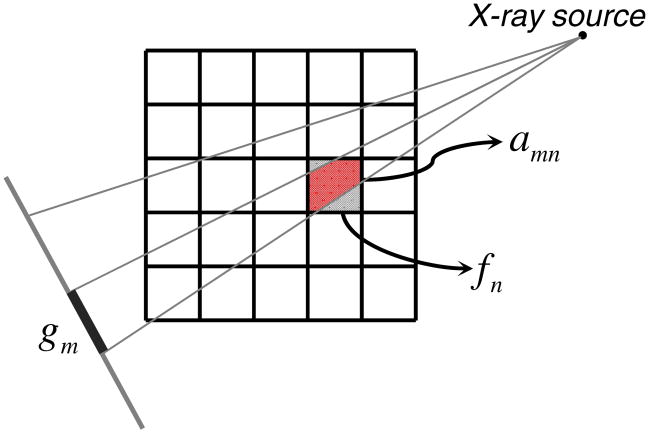
with 1 ≤ n ≤ N and N = I × J; we can re-arrange the image into a vector for the measurement model equation (2.1). In this paper, we will use both the signs f_i,j and f_n for convenience. Each component of the function g in equation (2.1) is a measured datum with M being the product of the number of projections and the number of detector elements. In a typical fan-beam geometry, the nth pixel can be viewed as a rectangular region with a constant value f_n, the mth measured datum g_m as an integral of areas of pixels partially covered by a narrow beam from an x-ray source to a detector element and weighted by the corresponding x-ray linear attenuation coefficients, respectively. Thus, the component a_m,n in equation (2.1) denotes the interaction area between the nth pixel and the mth fan-beam path (figure 2). While the whole matrix A represents the forward projection, A^T implements the back projection. The SART-type solution to equation (2.1) can be written as (Wang and Jiang 2004)

Figure 2.

Projection model of a discrete image in fan-beam geometry.

$$f_n^k=f_n^{k-1}+{\lambda }^k\frac{1}{a_{+n}}\sum _{m=1}^M\frac{a_{m,n}}{a_{m+}}(g_m-{\mathbf{A}}_m{\mathbf{f}}^{k-1}),$$ (3.2)

where $a_{+n}={\sum }_{m=1}^M{a}_{m,n}>0,a_{m+}={\sum }_{n=1}^N{a}_{m,n}>0$, A_m is the mth row of A, k is the iteration index and 0 < λ^k < 2 is a free relaxation parameter. Let Λ^+N ∈ ℝ^N × ℝ^N be a diagonal matrix with ${\mathbf{\Lambda }}_{nn}^{+N}=\frac{1}{a_{+n}}$ and Λ^M+ ∈ ℝ^M × ℝ^M be a diagonal matrix with ${\mathrm{\Lambda }}_{mm}^{M+}=\frac{1}{a_{m+}}$; equation (3.2) can be rewritten as f^k = f^k−1 + λ^k(Λ^+N A^T Λ^M+(g − Af^k−1)). This implies that the solution equation (3.2) corresponds to the inner item ‘f^k−1 + A^T (g − Af^k−1)’ in equation (2.6) with ${\mathbf{\Lambda }}_{nn}^{+N}$ and Λ^M+ being the weights for the normalization of the matrix A^T A, which can be used for a better converging behavior. To apply the soft-threshold algorithm subject to a sparsity constraint, we must find a suitable basis or frame ϕ_γ and (f), which is the major contribution of this paper.

3.2. Pseudo-inverse of the discrete gradient transform

In the medical imaging field, the DGT has been widely used to define a sparsity constraint. Let us assume that a digital image satisfies the so-called Neumann conditions on the boundary:

$$\begin{array}{llll}{f}_{0,j}=f_{1,j}\hfill & \text{and}\hfill & f_{I,j}=f_{I+1,j}\hfill & \text{for}1\le j\le J,\hfill \\ f_{i,0}=f_{i,1}\hfill & \text{and}\hfill & f_{i,J}=f_{i,J+1}\hfill & \text{for}1\le i\le I.\hfill \end{array}$$ (3.3)

Then, the standard isotropic discretization of TV can be expressed as

$$\begin{array}{c}TV(\mathbf{f})=\sum _{i=1}^I\sum _{j=1}^J{d}_{i,j},\\ d_{i,j}=\sqrt{{(f_{i,j}-f_{i+1,j})}^2+{(f_{i,j}-f_{i,j+1})}^2}.\end{array}$$ (3.4)

We re-write equation (2.4) for the CT reconstruction problem under the constraint of sparse gradient transform as

$${\mathrm{\Phi }}_{w,1}(\mathbf{f})=\mathrm{\Delta }(\mathbf{f})+2\mathit{wTV}(\mathbf{f}).$$ (3.5)

Since there does not exist a frame such that d_i,j = 〈f, ϕ_i,j〉, the solution equation (2.6) cannot be directly applied to minimize Φ_w,1(f) defined by equation (3.5). However, we can construct a pseudo-inverse of the DGT as follows. Assume that

$${\stackrel{\sim }{f}}_n^k=f_n^{k-1}+{\lambda }^k\frac{1}{a_{+n}}\sum _{m=1}^M\frac{a_{m,n}}{a_{m+}}(g_m-{\mathbf{A}}_m{\mathbf{f}}^{k-1})$$ (3.6)

is the update from the projection constraint in the current iteration step k, which is exactly the same as equation (3.2). We can compute

$$d_{i,j}^k=\sqrt{{({\stackrel{\sim }{f}}_{i,j}^k-{\stackrel{\sim }{f}}_{i+1,j}^k)}^2+{({\stackrel{\sim }{f}}_{i,j}^k-{\stackrel{\sim }{f}}_{i,j+1}^k)}^2}.$$ (3.7)

According to the soft-threshold operation in equation (2.9), when $d_{i,j}^k<w$, we can adjust the value of ${\stackrel{\sim }{f}}_{i,j}^k,{\stackrel{\sim }{f}}_{i+1,j}^k$ and ${\stackrel{\sim }{f}}_{i,j+1}^k$ to make $d_{i,j}^k=0$; and when $d_{i,j}^k\ge w$, we can reduce the values of ${({\stackrel{\sim }{f}}_{i,j}^k-{\stackrel{\sim }{f}}_{i+1,j}^k)}^2$ and ${({\stackrel{\sim }{f}}_{i,j}^k-{\stackrel{\sim }{f}}_{i,j+1}^k)}^2$ to perform the filtering. That is, we can construct the following pseudo-inverse (see the appendix for details of construction):

$$f_{i,j}^k=\frac{1}{4}(2f_{i,j}^{k,a}+f_{i,j}^{k,b}+f_{i,j}^{k,c}),$$ (3.8)

$$f_{i,j}^{k,a}=\{\begin{array}{ll}\frac{2{\stackrel{\sim }{f}}_{i,j}^k+{\stackrel{\sim }{f}}_{i+1,j}^k+{\stackrel{\sim }{f}}_{i,j+1}^k}{4},\hfill & \text{if}{d}_{i,j}^k<w\hfill \\ {\stackrel{\sim }{f}}_{i,j}^k-\frac{w(2{\stackrel{\sim }{f}}_{i,j}^k-{\stackrel{\sim }{f}}_{i+1,j}^k-{\stackrel{\sim }{f}}_{i,j+1}^k)}{4d_{i,j}^k},\hfill & \text{if}{d}_{i,j}^k\ge w,\hfill \end{array}$$ (3.9)

$$f_{i,j}^{k,b}=\{\begin{array}{ll}\frac{{\stackrel{\sim }{f}}_{i,j}^k+{\stackrel{\sim }{f}}_{i-1,j}^k}{2},\hfill & \text{if}{d}_{i-1,j}^k<w\hfill \\ {\stackrel{\sim }{f}}_{i,j}^k-\frac{w({\stackrel{\sim }{f}}_{i,j}^k-{\stackrel{\sim }{f}}_{i-1,j}^k)}{2d_{i-1,j}^k},\hfill & \text{if}{d}_{i-1,j}^k\ge w,\hfill \end{array}$$ (3.10)

$$f_{i,j}^{k,c}=\{\begin{array}{ll}\frac{{\stackrel{\sim }{f}}_{i,j}^k+{\stackrel{\sim }{f}}_{i,j-1}^k}{2},\hfill & \text{if}{d}_{i,j-1}^k<w\hfill \\ {\stackrel{\sim }{f}}_{i,j}^k-\frac{w({\stackrel{\sim }{f}}_{i,j}^k-{\stackrel{\sim }{f}}_{i,j-1}^k)}{2d_{i,j-1}^k},\hfill & \text{if}{d}_{i,j-1}^k\ge w.\hfill \end{array}$$ (3.11)

Equation (3.8) can be understood as a result of three consecutive steps. In the first step, the DGT $d_{i,j}^k$ is computed with respect to ${\stackrel{\sim }{f}}_{i,j}^k$; in the second step, a soft-threshold filtering is performed on $d_{i,j}^k$ to obtain ${\stackrel{\sim }{d}}_{i,j}^k$ and in the third step, an inverse DGT is constructed for ${\stackrel{\sim }{d}}_{i,j}^k$ with the prior information ${\stackrel{\sim }{f}}_{i,j}^k$. Because equation (3.8) serves as the inverse transform of ${\stackrel{\sim }{d}}_{i,j}^k$ in the soft-threshold filtering reconstruction framework, we call it a pseudo-inverse of the DGT. In summary, we have a soft-threshold algorithm for the TV minimization in the following pseudocode (figure 1(b)):

• S1Initialize the parameters k,w;
• S2Update the current reconstruction using equation (3.6);
• S3Perform the nonlinear filter using equation (3.8);
• S4Go to S2 until the stopping criterion is met.

3.3. Pseudo-inverse of the discrete difference transform

In addition to the DGT, there are other possible sparse transforms. For example, we can define a total difference (TD) of f as

$$\text{TD}(\mathbf{f})=\sum _{i=1}^I\sum _{j=1}^J{d}_{i,j},d_{i,j}=\mid f_{i,j}-f_{i+1,j}\mid +\mid f_{i,j}-f_{i,j+1}\mid$$ (3.12)

and rewrite equation (2.4) as

$${\mathrm{\Phi }}_{w,1}(\mathbf{f})=\mathrm{\Delta }(\mathbf{f})+2\mathit{wTD}(\mathbf{f}).$$ (3.13)

We call d_i,j in equation (3.12) a discrete difference transform (DDT). Similar to what we have done in subsection 3.2, after the soft-threshold filtering, we can construct a pseudo-inverse of $f_{i,j}^k$ as

$$f_{i,j}^k=\frac{1}{4}(q(w,{\stackrel{\sim }{f}}_{i,j}^k,{\stackrel{\sim }{f}}_{i+1,j}^k)+q(w,{\stackrel{\sim }{f}}_{i,j}^k,{\stackrel{\sim }{f}}_{i,j+1}^k)+q(w,{\stackrel{\sim }{f}}_{i,j}^k,{\stackrel{\sim }{f}}_{i,j-1}^k)+q(w,{\stackrel{\sim }{f}}_{i,j}^k,{\stackrel{\sim }{f}}_{i-1,j}^k)),$$ (3.14)

$$q(w,y,z)=\{\begin{array}{ll}\frac{y+z}{2},\hfill & \text{if}\mid y-z\mid <w\hfill \\ y-\frac{w}{2},\hfill & \text{if}(y-z)\ge w\hfill \\ y+\frac{w}{2},\hfill & \text{if}(y-z)\le -w.\hfill \end{array}$$ (3.15)

That is, we have a soft-threshold algorithm for TD minimization in the following pseudocode:

• S1Initialize the parameters k,w;
• S2Update the current reconstruction using equation (3.6);
• S3Perform the nonlinear filter using equation (3.14);
• S4Go to S2 until the stopping criterion is met.

4. Numerical simulations

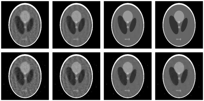
To demonstrate the validity of the proposed algorithms, we implemented them in MatLab and performed numerical tests. We assumed a circular scanning locus of radius 57.0 cm and fan-beam geometry. The object was a modified Shepp–Logan phantom in a compact support with a radius of 10.0 cm. We used an equi-distance virtual detector array of length 20.0 cm. The detector was centered at the system origin and made perpendicular to the direction from the origin to the x-ray source. The detector array consisted of 300 elements. For each of our selected number of projections over a full-scan range, we first equi-angularly acquired the corresponding projection dataset based on the discrete projection model shown in figure 2. Then, we reconstructed the images using the following four methods: (1) the classical SART iteration method without the regularization of sparsity, (2) the TV minimization algorithm implemented in Yu and Wang (2009) using the steepest descent search method, (3) the TV minimization algorithm with soft-threshold filtering proposed in subsection 3.2 and (4) the TD minimization method with soft-threshold filtering proposed in subsection 3.3. To accelerate the convergence, we employed the projected gradient method (Daubechies et al 2008) to determine an optimal threshold w for each filtering, which is similar to what we have done in Yu and Wang (2010). For all the above methods, the parameter λ^k in the SART iteration formula in equation (3.2) was set to be the constant 1.0, and the stopping criterion was defined as reaching the maximum iteration number 5000. Figures 3 and 4 show the reconstructed 256 × 256 images from 21 and 15 projections, respectively.

Figure 3.

Reconstructed images of a modified Shepp–Logan phantom from 21 projections after 5000 iterations. While the top-row images are from a noise-free dataset, the bottom-row images are from a dataset with Poisson noise. From left to right, the four columns are reconstructions using the SART method without TV minimization, the steepest descent method for TV minimization, the soft-threshold filtering methods for TV and TD minimization, respectively. The display window is [0, 0.5].

Figure 4.

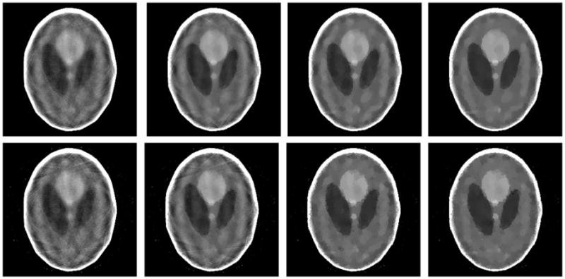
Counterparts of figure 3 from 15 projections.

For practical applications, measurement noise is unavoidable. To test the stability of the proposed algorithms against data noise, we repeated the aforementioned reconstructions from projections corrupted by Poisson noise, assuming 5 × 10⁴ photons per detector element (Yu et al 2006). The results are also shown in figures 3 and 4, which confirm the stability of the proposed algorithms.

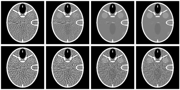
To challenge the proposed algorithms, we also repeated the aforementioned experiments using a low-contrast head phantom (http://www.imp.uni-erlangen.de/forbild/deutsch/results/head/head.html). Since the high-frequency and high-contrast fine inner ear structures cause severe artifacts overlapping with the low-contrast structures, we need more projections to reconstruct low-contrast structures well. Hence, we simulated the cases of 61 and 41 projections and assumed 5×10⁵ photons per detector element for the low-dose datasets. The corresponding results are in figures 5 and 6.

Figure 5.

Reconstructed images of a FORBILD head phantom from 61 projections after 5000 iterations. While the top-row images are from a noise-free dataset, the bottom-row images are from a dataset with Poisson noise. From left to right, the four columns are reconstructions using the SART method without TV minimization, the steepest descent method for TV minimization, the soft-threshold filtering methods for TV and TD minimization, respectively. The display window is [1.0, 1.1].

Figure 6.

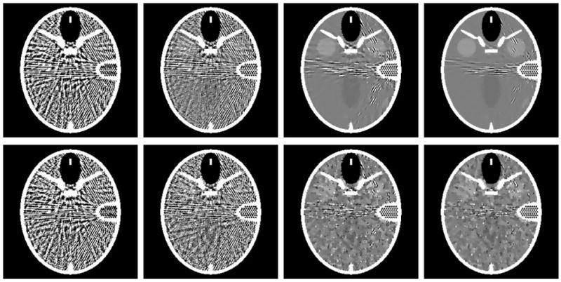
Counterparts of figure 5 from 41 projections.

5. Discussions and conclusion

Because the DGT and DDT are not invertible, they do not satisfy the requirement of the CS theory and the soft-threshold algorithm, both of which assume the transform is invertible. In this paper, we have constructed two pseudo-inverse transforms (equations (3.8) and (3.14)) to address this issue. Different from the truly invertible transforms, these pseudo-inverses take advantage of reconstructed images from the previous iteration. Although these inverses may still not have the RIP, they can now be fitted in the soft-threshold filtering reconstruction framework and indeed produced excellent reconstruction results. Clearly, pseudo-inverse transforms can also be regarded as nonlinear filters. However, we prefer to call them pseudo-inverse transforms because they serve as the inverse transforms of the DGT and DDT, respectively, after the soft-threshold filtration defined by equation (2.6) in the soft-threshold filtering framework.

Theoretically speaking, if available projections satisfy the exact reconstruction condition according to the CS theory (Donoho 2006, Candes et al 2006), all the aforementioned reconstruction algorithms can converge to the desired solution. In other words, for any given dataset, the larger the total number of iterations, the better the reconstructed image quality. This point is illustrated in figure 7. However, their convergence speeds are different. For a given iteration number 5000, figures 3–6 show that the proposed TV and TD minimization methods outperform the traditional steepest descent search method. Meanwhile, the TD minimization is not only simpler for practical implementation but also performs slightly better than the TV minimization. Therefore, we believe that the TD minimization proposed in this paper should have practical applications.

Figure 7.

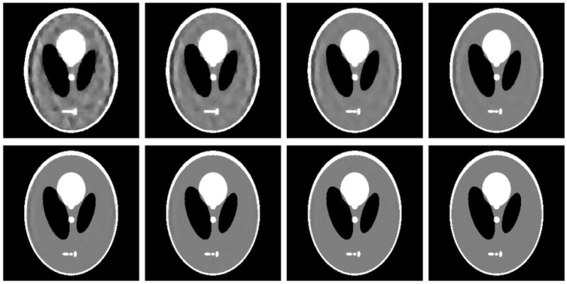
Reconstructed images of a modified Shepp–Logan phantom from 21 noise-free projections after different numbers of iterations. From top to bottom and from left to right, the number of iterations for the first seven images are 500, 1000, 2000, 4000, 6000, 8000 and 10 000, respectively. As the benchmark, the last image is the ideal phantom image. The display window is [0.15, 0.25].

In the review process of this manuscript, the level-set-based method for TV minimization (Marquina and Osher 2000, Yu et al 2005) was brought to our attention. The idea of this methodology is to convert the constrained CT reconstruction problem to a time-dependent partial differential equation (equations (2.6) & (2.7) in Yu et al (2005)). From the viewpoint of numerical implementation, equation (2.6) in Yu et al (2005) can be regarded as a one-step iteration for the inner steepest descent search implemented in Yu and Wang (2009). Due to the introduction of |∇u| in equation (2.7) in Yu et al (2005), the level-set-based method can be viewed as an accelerated version of the commonly used steepest search method (Yu and Wang 2009). Similar to other optimization problems, the reconstruction results highly depend on the choice of the relax parameter λ. On the other hand, the pseudo-inversions suggested in this paper are constructed using the soft-threshold filtering method. Using the projected gradient technique, the threshold in each filtering step is automatically determined, and the iterative sequence converges to the solution that minimizes the objective function. Comparative studies in this direction will be pursued in the future.

At the gallery proof stage, on the first international meeting on image formation in x-ray computed tomography in Salt Lake City, Dr Jeffrey Fessler brought our attention to the work on super resolution by Farsiu et al (2004), in which they defined bilateral total variation (BTV) as a regularizer. The TD (total difference) defined in this paper is a special case of BTV. Also, TD was suggested as a reliable and computationally efficient approximation to the TV by others (Li and Santosa 1996) in the image processing field. Here it has been shown that TD performs even better than TV in our simulation setting.

In conclusion, we have constructed a pseudo-inverse of the DGT and a pseudo-inverse of the DDT to apply the soft-threshold filtering principle for image reconstruction subject to a sparsity constraint. In the spirit of the above-described strategy for algorithm construction, we can derive a variety of algorithms of this type. In the near future, we will investigate and evaluate other reconstruction schemes with numerical, physical, preclinical and clinical datasets.

Appendix. Construction of the pseudo-inverse of DGT

To simplify the notation, as shown in figure A1, we only consider the discrete gradient

Figure A1.

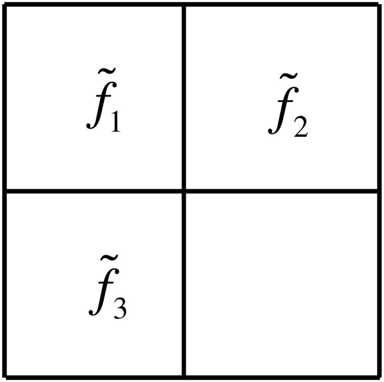
Neighborhood pixels used in equation (A.1).

$$d=\sqrt{{({\stackrel{\sim }{f}}_1-{\stackrel{\sim }{f}}_2)}^2+{({\stackrel{\sim }{f}}_1-{\stackrel{\sim }{f}}_3)}^2}.$$ (A.1)

Case I: d < w

When d < w, the soft-thresholding operation requires to adjust the values of f̃₁, f̃₂ and f̃₃ to make d = 0. Because equation (A.1) implies that f̃₁ − f̃₂ = 0 when d = 0, we can assign the new value $f_1=f_2=\frac{{\stackrel{\sim }{f}}_1+{\stackrel{\sim }{f}}_2}{2}$ to satisfy f̃₁ − f̃₂ = 0. Similarly, we can assign the new value $f_1=f_3=\frac{{\stackrel{\sim }{f}}_1+{\stackrel{\sim }{f}}_3}{2}$ to satisfy f̃₁ − f̃₃ = 0. However, $f_1=\frac{{\stackrel{\sim }{f}}_1+{\stackrel{\sim }{f}}_2}{2}$ and $f_1=\frac{{\stackrel{\sim }{f}}_1+{\stackrel{\sim }{f}}_3}{2}$ are inconsistent. Hence, we can use their average as the final adjustment. That is, we have

$$\{\begin{array}{l}{f}_1=\frac{2{\stackrel{\sim }{f}}_1+{\stackrel{\sim }{f}}_2+{\stackrel{\sim }{f}}_3}{4}\hfill \\ f_2=\frac{{\stackrel{\sim }{f}}_1+{\stackrel{\sim }{f}}_2}{2}\hfill \\ f_3=\frac{{\stackrel{\sim }{f}}_1+{\stackrel{\sim }{f}}_3}{2}.\hfill \end{array}$$ (A.2)

Case II: d ≥ w

When d ≥ w, the soft-thresholding operation requires to adjust the values of f̃₁, f̃₂ and f̃₃ for d to become d − w. For this purpose, we use a multiplicative factor $\beta =\frac{d-w}{d}$ and obtain

$$d-w=\sqrt{{({\stackrel{\sim }{f}}_1-{\stackrel{\sim }{f}}_2)}^2{\beta }^2+{({\stackrel{\sim }{f}}_1-{\stackrel{\sim }{f}}_3)}^2{\beta }^2}.$$ (A.3)

This implies that we can set |f₁ − f₂| = β|f̃₁ − f̃₂| and |f₁ − f₃| = β|f̃₁ − f̃₃|. To satisfy |f₁ − f₂| = β|f̃₁ − f̃₂|, one possible way is to assign

$$\{\begin{array}{l}{f}_1={\stackrel{\sim }{f}}_1-\frac{(1-\beta )({\stackrel{\sim }{f}}_1-{\stackrel{\sim }{f}}_2)}{2}={\stackrel{\sim }{f}}_1-\frac{w({\stackrel{\sim }{f}}_1-{\stackrel{\sim }{f}}_2)}{2d}\hfill \\ f_2={\stackrel{\sim }{f}}_2-\frac{(1-\beta )({\stackrel{\sim }{f}}_2-{\stackrel{\sim }{f}}_1)}{2}={\stackrel{\sim }{f}}_2-\frac{w({\stackrel{\sim }{f}}_2-{\stackrel{\sim }{f}}_1)}{2d}.\hfill \end{array}$$ (A.4)

Similarly, we can assign

$$\{\begin{array}{l}{f}_1={\stackrel{\sim }{f}}_1-\frac{(1-\beta )({\stackrel{\sim }{f}}_1-{\stackrel{\sim }{f}}_3)}{2}={\stackrel{\sim }{f}}_1-\frac{w({\stackrel{\sim }{f}}_1-{\stackrel{\sim }{f}}_3)}{2d}\hfill \\ f_3={\stackrel{\sim }{f}}_3-\frac{(1-\beta )({\stackrel{\sim }{f}}_3-{\stackrel{\sim }{f}}_1)}{2}={\stackrel{\sim }{f}}_3-\frac{w({\stackrel{\sim }{f}}_3-{\stackrel{\sim }{f}}_1)}{2d}.\hfill \end{array}$$ (A.5)

to satisfy |f₁ − f₃| = β|f̃₁ − f̃₃|. Again, due to the inconsistency between the values of f₁ in (A.4) and (A.5), we take their average and obtain

$$\{\begin{array}{l}{f}_1={\stackrel{\sim }{f}}_1-\frac{w(2{\stackrel{\sim }{f}}_1-{\stackrel{\sim }{f}}_2-{\stackrel{\sim }{f}}_3)}{4d}\hfill \\ f_2={\stackrel{\sim }{f}}_2-\frac{w({\stackrel{\sim }{f}}_2-{\stackrel{\sim }{f}}_1)}{2d}\hfill \\ f_3={\stackrel{\sim }{f}}_3-\frac{w({\stackrel{\sim }{f}}_3-{\stackrel{\sim }{f}}_1)}{2d}.\hfill \end{array}$$ (A.6)

We can obtain the weighted mean equation (3.8) from equations (A.2) and (A.6).

References

- Candes EJ, Romberg J, Tao T. Robust uncertainty principles: exact signal reconstruction from highly incomplete frequency information. IEEE Trans Inf Theory. 2006;52:489–509. [Google Scholar]
- Chen GH, Tang J, Leng S. Prior image constrained compressed sensing (PICCS): a method to accurately reconstruct dynamic CT images from highly undersampled projection data sets. Med Phys. 2008;35:660–3. doi: 10.1118/1.2836423. [DOI] [PMC free article] [PubMed] [Google Scholar]
- Daubechies I, Defrise M, De Mol C. An iterative thresholding algorithm for linear inverse problems with a sparsity constraint. Commun Pure Appl Math. 2004;57:1413–57. [Google Scholar]
- Daubechies I, Fornasier M, Loris I. Accelerated projected gradient method for linear inverse problems with sparsity constraints. J Fourier Anal Appl. 2008;14:764–92. [Google Scholar]
- Donoho DL. Compressed sensing. IEEE Trans Inf Theory. 2006;52:1289–306. [Google Scholar]
- Farsiu S, et al. Fast and robust multiframe super resolution. IEEE Trans Image Process. 2004;13:1327–44. doi: 10.1109/tip.2004.834669. [DOI] [PubMed] [Google Scholar]
- Figueiredo MAT, Nowak RD. An EM algorithm for wavelet-based image restoration. IEEE Trans Image Process. 2003;12:906–16. doi: 10.1109/TIP.2003.814255. [DOI] [PubMed] [Google Scholar]
- Li Y, Santosa F. A computational algorithm for minimizing total variation in image restoration. IEEE Trans Image Process. 1996;5:987–95. doi: 10.1109/83.503914. [DOI] [PubMed] [Google Scholar]
- Marquina A, Osher S. Explicit algorithms for a new time dependent model based on level set motion for nonlinear deblurring and noise removal. SIAM J Sci Comput. 2000;22:387–405. [Google Scholar]
- Rudin LI, Osher S, Fatemi E. Nonlinear total variation based noise removal algorithms. Physica D. 1992;60:259–68. [Google Scholar]
- Sidky EY, Kao CM, Pan XC. Accurate image reconstruction from few-views and limited-angle data in divergent-beam CT. J X-Ray Sci Technol. 2006;14:119–39. [Google Scholar]
- Tang J, Nett BE, Chen GH. Performance comparison between total variation (tv)-based compressed sensing and statistical iterative reconstruction algorithms. Phys Med Biol. 2009;54:5781–804. doi: 10.1088/0031-9155/54/19/008. [DOI] [PMC free article] [PubMed] [Google Scholar]
- Wang G, Jiang M. Ordered-subset simultaneous algebraic reconstruction techniques (OS-SART) J X-ray Sci Technol. 2004;12:169–77. [Google Scholar]
- Yu GQ, et al. Total variation based iterative image reconstruction. In: Liu Y, Jiang T, Zhang CS, editors. Proc Computer Vision for Biomedical Image Applications. 2005. pp. 526–34. [Google Scholar]
- Yu HY, Wang G. Compressed sensing based interior tomography. Phys Med Biol. 2009;54:2791–805. doi: 10.1088/0031-9155/54/9/014. [DOI] [PMC free article] [PubMed] [Google Scholar]
- Yu HY, Wang G. SART-type image reconstruction from a limited number of projections with the sparsity constraint. Int J Biomed Imaging. 2010;2010:934847. doi: 10.1155/2010/934847. [DOI] [PMC free article] [PubMed] [Google Scholar]
- Yu HY, et al. Local ROI reconstruction via generalized FBP and BPF algorithms along more flexible curves. Int J Biomed Imaging. 2006;2006:14989. doi: 10.1155/IJBI/2006/14989. [DOI] [PMC free article] [PubMed] [Google Scholar]