Combining Steady-State and Dynamic Methods for Determining Absolute Signs of Hyperfine Interactions: Pulsed ENDOR Saturation and Recovery (PESTRE)

Abstract

The underlying causes of asymmetric intensities in Davies pulsed ENDOR spectra that are associated with the signs of the hyperfine interaction are reinvestigated. The intensity variations in these asymmetric ENDOR patterns are best described as shifts in an apparent baseline intensity that occurs dynamically following on-resonance ENDOR transitions. We have developed an extremely straightforward multi-sequence protocol that is capable of giving the sign of the hyperfine interaction by probing a single ENDOR transition, without reference to its partner transition. This technique, Pulsed ENDOR Saturatation and Recovery (PESTRE) monitors dynamic shifts in the ‘baseline’ following measurements at a single RF frequency (single ENDOR peak), rather than observing anomalous ENDOR intensity differences between the two branches of an ENDOR response. These baseline shifts, referred to as dynamic reference levels (DRLs), can be directly tied to the electron spin manifold from which that ENDOR transition arises. The application of this protocol is demonstrated on ⁵⁷Fe ENDOR of a 2Fe-2S ferredoxin. We use the ¹⁴N ENDOR transitions of the S = 3/2 [Fe(II)NO]²⁺ center of the non-heme iron enzyme, anthranilate dioxygenase (AntDO) to examine the details of the relaxation model using PESTRE.

Introduction

Recent studies have demonstrated that under certain conditions it is possible to extract the absolute signs of hyperfine interactions (HFI) from electron-nuclear double resonance (ENDOR) experiments. [1] It has long been known that this is possible for high-spin systems if one can measure the pseudonuclear Zeeman effect, a difference between the expected and observed nuclear Zeeman frequency, ν_N. [2] More generally, and more recently, procedures to extract HFI signs have been developed based on the observation of ‘anomalous’ (vide infra) ENDOR intensity differences between the two ENDOR branches, denoted ν₊ and ν₋, of an I=1/2 nucleus hyperfine-coupled to a S=1/2 spin. Bennebroek and Schmidt[1] first provided an explanation of intensities in the pulsed Mims ENDOR spectra of ¹⁰⁷Ag and ¹⁰⁹Ag obtained at 95 GHz and 1.2K for self-trapped hole complexes in AgCl crystals. Their key insight was that HFI sign information is dynamically impressed on the electron-spin-echo (ESE) response producing ν₊/ν₋ intensity asymmetries of ENDOR spectra, through the effects of spin relaxation and electron-spin polarization. Epel et al. [3] extended this work to a wider range of experimental conditions in Davies ENDOR experiments. They described how various regimes of relaxation rates (times) W₁ = T₁⁻¹, W_X = T_X⁻¹, and W_N = T_N⁻¹ (defined in Fig. 1) combined with variations in pulse intervals, t_Mix and t_Wait (defined in Fig. 2) lead to anomalous/unequal steady-state Davies ENDOR intensities for the two ENDOR transitions that can be analyzed to yield hyperfine signs. Subsequent papers by Yang and Hoffman[4] and Morton et al. [5] extended the work of Epel et al. to focus on super/multi-sequence effects where the anomalous steady-state intensities within a spectrum are generated through pulse multi-sequences rather than the earlier focus on the timing intervals within a single sequence. Morton et al. provide suggestions regarding the relative efficacies of the various techniques in samples with different relaxation characteristics.

FIG 1.

Upper: Energy level diagram for the S=1/2, I=1/2 spin system with EPR and NMR transitions. Lower: Relaxation pathways and rate constant labels for the electron spin lattice relaxation (W₁ = T₁⁻¹), electron-nuclear cross relaxation (W_X = T_X⁻¹) and nuclear relaxation mechanisms (W_N = T_N⁻¹).

FIG 2.

Davies ENDOR pulse sequence diagram with definitions of t_Mix, t_Wait, and t_R.

The techniques covered by Epel et al., Yang and Hoffman, and Morton et al. employ traditional ‘swept’ Davies ENDOR measurements in which a spectrum is generated by collecting and summing/averaging the echoes from one or more ENDOR sequences for a given radio frequency (RF) and then incrementing/decrementing the RF to the adjacent frequency, repeating this process sequentially across the desired RF range. To improve the S/N ratio, multiple scans are collected by repeating this process. ENDOR intensities in the resulting spectra are measured by comparing the averaged echo intensities collected when the RF is on-resonance with an NMR transition to that for a ‘baseline’ value obtained when the RF is off-resonance for all NMR transitions. Intensities in such spectra are called anomalous when the relative intensities of the ν₊/ν₋ transitions thus defined differ from those predicted by Boltzmann intensity factors.

One important limitation of these procedures is that they require the observation of both ν₊ and ν₋ branches of the spectrum, and often this is not feasible, for example because of overlap or in the case where ν₋→0. Of far greater significance, all of these procedures fail in the numerous cases where spectra include not merely intensity anomalies for well-defined ν₊/ν₋ pairs but also major distortions, such as the appearance of negative and positive ENDOR responses, and where the behavior depends on the sweep direction. These distortions can be so severe that there is no well-defined ‘baseline’ and it is impossible even to determine the frequencies of the underlying NMR transitions. Observation of these types of relaxation artifacts in packet-shifting ENDOR measurements dates back to the original paper of Feher.[6] One example of this extreme type of anomalous ENDOR spectrum is shown in Fig. 3, which presents the Davies ENDOR response of the ⁵⁷Fe ions in a 2Fe-2S ferredoxin as recorded at 35 GHz and 2 K at a field position between g₁ (2.025) and g₂ (1.938). The low-to-high (plus) and high-to-low (minus) linear sweeps have regions in the spectra that are positive for one direction and negative for the other, relative to the off-resonance baseline. For the frequency marked with an ‘*’, a peak maximum in the plus-direction scan (top) actually corresponds to a peak minimum in the minus direction scan (middle). Such sweep distortions can be eliminated (Fig. 3, bottom) by using random-hop RF excitation, [7; 8] which is a variation of the stochastic ENDOR approach suggested by Bruggemann and Niklas.[9] For example, note that the (*) peak corresponds to the maximum ENDOR intensity in the randomly-hopped spectrum. The spectrum can now be assigned as a pair of peaks at lower frequency assigned to the Fe(II) ion site and an orientation-selective pattern for the Fe(III) ion due to a rotation of the hyperfine tensor relative to the g tensor. A more extensive discussion of these assignments is given in section VI. The price of the random-hopped protocol is that it eliminates all anomalous ENDOR intensities, and therefore hides the much-desired hyperfine sign information.

FIG 3.

⁵⁷Fe Davies ENDOR spectra of a 2Fe-2S cluster at 35 GHz and 2K showing the effects of sweep artifacts on the appearance of the spectra. The top two panels are RF-frequency swept low-to-high (upper) and high-to-low (lower). The bottom panel shows the improvement obtained via random-hopping of the RF excitation frequency. Conditions: microwave frequency 34.79 GHz, magnetic field, 1259 mT, microwave pulse lengths, 120 ns, 60 ns, 120 ns, RF pulse length 30 μs, repetition time 100 ms.

We now present a new approach to the study of how relaxation effects lead to anomalous intensities in swept ENDOR spectra. By combining aspects of both the dynamic and steady-state approaches, we find that HFI signs are most robustly measured by monitoring the return of the ESE intensity to its RF-off steady-state (‘baseline’) value during a train of ESE sequences without RF that follows a train of Davies sequences with on-resonance NMR pulses at a fixed frequency. Literally, this method involves studying sweep artifacts, such as those described in Fig. 3, rather than the ENDOR itself. The new experimental protocol, denoted Pulsed ENDOR Saturation and Recovery (PESTRE), produces intensity signatures that are easily correlated with the anomalous ENDOR intensities and can be used to assign hyperfine signs unambiguously even when only a single branch of the ENDOR pattern is observable. This alone is a major advance, as all previous techniques require a comparison either of the frequencies or intensities of ν₊/ν₋ pairs. In addition, we are able to explain the nature of anomalous ENDOR intensities and provide a more precise method to measure the rates of nuclear/cross relaxation. It will be seen that a key step in developing this approach is a precise definition of multiple ESE and ENDOR ‘baselines’. To demonstrate the PESTRE experiment, PESTRE traces are measured for two of the ⁵⁷Fe peaks from the 2Fe-2S center whose ENDOR spectrum is shown Fig. 3. To test the model of the PESTRE protocol, we reexamine the relaxation characteristics[4; 5] of the S = 3/2 [Fe(II)NO]²⁺ center of the non-heme iron enzyme, anthranilate dioxygenase (AntDO).[10]

II. Modelling the Davies ENDOR response

A. Formulation

The frequencies of the two ENDOR transitions in a S=1/2, I=1/2 coupled system are given to first-order by

$${\nu }_{\pm }=\mid g_N{\beta }_N{B}_0-M_{S}A\mid$$ [1]

where |g_Nβ_NB₀| is the Larmor frequency (ν_N) of the nucleus at the observing static field B₀; ν₊ always refers to the peak at the higher NMR frequency and ν₋ to the lower-frequency transition, regardless of the sign of A. In the absence of any additional information, the sign of A cannot be determined from knowledge of these two frequencies. The question, ‘What is the sign of A?’, instead is answered by determining which of the ν₊/ν₋ transitions is associated with the β (M_S = −1/2; lower energy) electron-spin (ES) manifold of electron-nuclear states and which transition with α (M_S = +1/2).

A standard Davies ENDOR pulse sequence [11] (Fig. 2) consists of a selective microwave pulse of strength B₁ and length t_p, a subsequent selective RF pulse applied during a mixing period (t_Mix), then an electron-spin Hahn-echo detection sequence (t_p-τ-2t_p-τ-echo). In the course of a typical experimental ENDOR protocol, an individual Davies ENDOR sequence follows the preceding one after a waiting period, t_Wait, which is typically on the order of the electron spin-lattice relaxation time, T₁. The microwave pulses are on the order of tens of nanoseconds, the RF pulse applied during the mixing period, t_Mix, is on the order of tens of microseconds, and t_Wait is often on the order of milliseconds or longer. The mixing period can be as short as the RF pulse length itself and up to the millisecond time scale. Under these conditions, the total time for a single Davies pulse sequence (t_R) is approximately given by t_Wait + t_Mix. It is the dynamics of the spin relaxation during these two time periods, t_Wait and t_Mix, that creates the anomalous ENDOR intensities and allows the HFI sign to be obtained.

As described both in Bennebroek and Schmidt[1] and Epel et al., [7] modeling ESE responses for a four-state S = 1/2, I = 1/2 spin system during an ideal Davies ENDOR experiment only requires computation of the diagonal elements of the density matrices, which can be expressed as the fractional populations (n_i) of the four eigenstates of the <M_S,M_I| in a static field as shown in figure 1. In this approach, these populations are expressed as a column vector, n = (n₁,n₂,n₃,n₄)^T where Σn_i =1, the microwave and RF pulses and relaxation intervals correspond to 4×4 propagator matrices, and the electron and nuclear relaxation is treated with a master-equation approach. In any ESE experiment in which the inhomogenous EPR linewidth exceeds the hyperfine splitting, which is typical for metalloproteins, the ESE response must be modeled by summing over all possible allowed EPR transitions separately. For a S=1/2, I = 1/2 case, this is trivial as under most realistic circumstances, the ESE responses from the two EPR lines are identical.

Following Bennebroek and Schmidt,[1] we find that for the 4-state S=1/2 I=1/2 system, there are advantages to describing the anomalous ENDOR effects with the column vector,

$$\mathbf{\sigma }=\left[\begin{array}{c}E\\ S_Z\\ 2S_Z{I}_Z\\ I_Z\end{array}\right]$$ [2]

whose components are the expectation values of the four corresponding longitudinal product-operators (PO) [1; 12] and which are related to the eigenstate populations of (n_i) as follows:

$$\begin{array}{ccc}\text{E}=\frac{1}{2}(n_1+n_2+n_3+n_4)\equiv \frac{1}{2}& :& {\text{S}}_{\text{Z}}=\frac{1}{2}(n_1-n_2+n_3-n_4)\\ 2{\text{S}}_{\text{Z}}{\text{I}}_{\text{Z}}=\frac{1}{2}(n_1-n_2-n_3+n_4)& :& {\text{I}}_{\text{Z}}=\frac{1}{2}(n_1+n_2-n_3-n_4)\end{array}$$ [3]

The propagator matrices for the pulses this PO basis are given in the Appendix. We consider an ideal Davies ENDOR experiment in which the hyperfine-field splitting B_A = |A/g_eβ_e|, is much greater than the microwave excitation field, B₁. Under these conditions, the microwave pulses can be considered perfectly selective, so that when either EPR₁ or EPR₂ transition (figure 1, upper) matches the microwave quantum, the other EPR transition is unaffected by the pulse. This leads the propagators for the microwave pulses with turning angle of π (P₁) and a detection sequence π/2-π (P₂₃) as defined in the Appendix Eq. [A20] Similarly, the NMR-π pulses are considered to be perfectly selective, so that only one of the two NMR transitions can be resonant at any frequency. The propagators for the two resonant NMR π-pulses for the M_S=+1/2 and M_S=−1/2 manifolds respectively are P_RF^α and P_RF^β as given in Eq. [A21]. For Davies ENDOR sequences without a resonant NMR pulse, the NMR propagator can be replaced by the identity matrix, P_I.

The Davies 2-pulse detection sequence can be thought of as reporting the population difference that exists across the on-resonance EPR transition prior to the application of the 2^nd and 3^rd pulses of that Davies sequence. We denote this difference as the ESE intensity function Sig(σ) which takes on a value that depends on the resonant EPR transition

$$\mathit{Sig}(\mathbf{\sigma })=\{\begin{array}{ccc}{S}_Z+2S_Z{I}_Z=n_1-n_2& :& {\text{EPR}}_1\\ S_Z-2S_Z{I}_Z=n_3-n_4& :& {\text{EPR}}_2\end{array}$$ [4]

B. Relaxation Matrix

When dealing with relaxation that occurs within a single sequence and time intervals that are short relative to the cross/nuclear relaxation times such, as in the VMT-ENDOR protocol when it is combined with random-hopping of the RF, [13] the original description provided by Bennebroek and Schmidt[1] is sufficient to describe the anomalous ENDOR effects. This simple model utilizes the differences in the observed polarizations that are created by T₁ relaxation following an NMR pulse to describe the time evolution of the observed in ENDOR asymmetries when the mixing time is increased to values that are on the order of T₁.

Measurements involving multi-sequence ESE/ENDOR require descriptions of saturation behaviors and sweep artifacts as well as times intervals that are long relative to T₁. In these cases, the more elaborate electron-nuclear spin relaxation model presented by Epel et al. [7] (figure 1 lower) is required to account for all relaxation pathways and all time scales. In this approach, the propagators, P_tWait and P_tMix for the two relaxation intervals, t_Wait and t_Mix respectively, are modeled mathematically through a master-equation approach written in terms of the population vector, n = (n₁,n₂,n₃,n₄)^T. We find that it is easier to describe the intensities of the dynamic baseline shifts by using the PO basis since these intensities are tied directly to the value of a single component (I_Z) in this basis as described in section V. Transformation of the previously reported 4×4 master relaxation matrix Γ_n to PO basis leads to a master equation for σ

$$\frac{d\mathbf{\sigma }}{dt}=-{\mathbf{\Gamma }}_{\mathbf{\sigma }}\mathbf{\sigma }$$ [5]

where Γ_σ is block-diagonal in 2×2 blocks (E, S_Z) and (2S_ZI_Z, I_Z)

$${\mathbf{\Gamma }}_{\mathbf{\sigma }}=\left[\begin{array}{cccc}0& 0& 0& 0\\ -(W_x+W_1)(2f_{-}-1)& W_X+W_1& 0& 0\\ 0& 0& W_1+W_N& -(2f_{-}-1)W_1\\ 0& 0& -(2f_{-}-1)W_x& W_x+W_N\end{array}\right]$$ [6]

where $W_1=\frac{1}{T_1},W_X=\frac{1}{T_X},W_N=\frac{1}{T_N}$ and $f_{-}=\frac{exp\left(h\nu /k_{B}T\right)}{1+exp\left(h\nu /k_{B}T\right)}$, the fraction of spins in the M_S = −1/2 manifold at thermal equilibrium. For reference, in a spectrometer operating at (9.5 GHz, 35 GHz, and 95 GHz), the f₋ is (0.51, 0.55, 0.64) at 8 K, (0.53, 0.60, 0.75) at 4.2 K, and (0.55, 0.70, 0.90) at 2 K.

Given σ(t), for any relaxation time interval, Δt, value of σ(t+Δt) is then

$$\begin{array}{l}\mathbf{\sigma }(t+\mathrm{\Delta }t)=[\mathbf{VR}·\mathbf{exp}(-\mathbf{\Lambda }\mathbf{\Delta }\mathbf{t})·\mathbf{VL}]\mathbf{\sigma }(t)\\ =[{\mathbf{P}}_{\mathrm{\Delta }t}]\mathbf{\sigma }(t)\end{array}$$ [7]

where VL, VR are the left- and right- eigenvector matrices of Γ_σ and exp(−ΛΔt) is a diagonal matrix, D where D_mm = exp(−λ_mΔt) and λ_m are the eigenvalues (characteristic relaxation rates) of Γ_σ. The exact eigenvalues (λ_m) and left- and right-eigenvectors (VL_m, VR_m) for Γ_σ are easily obtained via standard methods and these exact solutions are used for all calculations in this paper. The matrix, P_Δt, propagates the spin system during a relaxation interval, Δt. We denote P_Δt as the relaxation matrix, and describe individual elements within this matrix as pδ_lm.

For comparisons to approximate solutions given by Epel et al. [3] we give the eigenvalues and eigenvectors correct to first-order in the limit that W₁≫W_X, W_N, (T₁≪T_X, T_N) and f₋ ≠ 0.5

$$\begin{array}{lll}{\lambda }_1=0\hfill & :\hfill & {\mathbf{VR}}_{\mathbf{1}}={\left(1+{(2f_{-}-1)}^2\right)}^{\frac{-1}{2}}{(1,2f_{-}-1,0,0)}^T\hfill \\ {\lambda }_2=W_1+W_X\hfill & :\hfill & {\mathbf{VR}}_{\mathbf{2}}={(0,1,0,0)}^T\hfill \\ {\lambda }_3=W_1+W_N+\frac{W_X{(2f_{-}-1)}^2}{W_1-W_X}\hfill & :\hfill & {\mathbf{VR}}_{\mathbf{3}}=N_3{\left(0,0\frac{W_1-W_X}{W_X(2f_{-}-1)},-1\right)}^T\hfill \\ {\lambda }_4=W_N+W_X-\frac{W_X{(2f_{-}-1)}^2}{W_1-W_X}\hfill & :\hfill & {\mathbf{VR}}_{\mathbf{4}}=N_4{\left(0,0\frac{W_1(2f_{-}-1)}{W_1-W_X},1\right)}^T\hfill \end{array}$$ [8]

where N₃ and N₄ are normalization constants and VR_m refers to m^th right-eigenvector. These approximate solutions do not require large thermal polarizations, (f₋≫0.5), merely that f₋≠ 0.5 when W₁ ≪ W_X, W_N, i.e., the ‘slow relaxation regime.’ We will discuss the physical interpretations of the eigenvectors and the relaxation matrix in Section V.

C. Extension to I>1/2

The S=1/2, I=1/2 model has been extended analytically to I>1/2 nuclei through a simple reworking of the propagators and relaxation matrices and we present a comparison of PESTRE traces for the I=1 to the I=1/2 system in the supplement. However, discussion of this extension is unnecessary and overly complex as a simple phenomenological picture explains why an I=1/2 analysis is valid model for I>1/2 nuclei in systems for which anomalous ENDOR intensities are observable. We use an S=1/2, I=1 system as an example. The six energy levels define three EPR transitions and four NMR transitions as shown in Fig. 4. Implicit in any Davies ENDOR experiment is that the microwave excitation is selective, namely, B₁ < |A/g_eβ_e|, so that only one of the three EPR transitions is being probed at a time. When there is resolved quadrupole splitting, then there are four different NMR transition frequencies, and the RF pulses are therefore also selective. Each NMR transition connects only two EPR transitions, either EPR₁ + EPR₂ or EPR₂ + EPR₃, leaving the third EPR transition unaffected. Thus, the six-level system separates into two overlapping four-level systems, shown by the boxes in the Fig. 4, and each can be mapped directly to an effective I′ =1/2 model for the microwave and NMR pulses.

FIG 4.

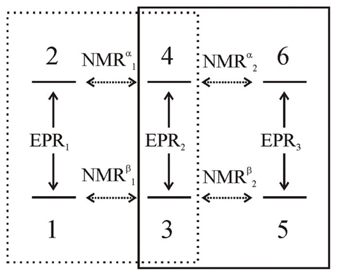
Diagram of a six-level S=1/2, I=1 system showing that the ENDOR measurements on (NMR^α₁, NMR^β₁) or (NMR^α₂, NMR^β₂) can approximated by a four-level, I′ =1/2 model. The two overlapping 4-level systems are outlined in the boxes.

To complete the mapping, note that when considering anomalous ENDOR intensities, the model assumes that the relaxation within the states that define each of the EPR transitions, the electron spin lattice relaxation, T_1, is rapid when compared to the relaxation between the states of different EPR transitions, as determined by T_X and T_N. Mathematically, this means that in any ENDOR experiment, the populations of the ‘additional’ two states not associated with the ‘active’ EPR transitions are only weakly coupled to the populations of the four states that are active in the ENDOR experiment and at most need to be treated by simple perturbation methods. The same argument can then be extended to any higher nuclear spin nucleus by the same logic.

III. Multi-Sequence Davies ENDOR

A. Baselines

In order to explore the dynamic changes in an EPR signal that occur during a multi-sequence at a fixed RF frequency, we start by defining the ESE signal for a single Davies sequence (j) within a Davies multi-sequence, Davies(t_Mix, t_Wait, RF^M)_j (Fig. 2), where M denotes the electron-spin manifold of a resonant NMR transition: M = α or β, or M = I (identity propagator) for a sequence without on-resonance RF. The ESE for the j^th sequence depends on the spin polarization resultant of all previous (j−1) sequences, as embodied by the polarization vector, σ_j−1 at the end of the sequence (j−1), and is given by the equation (see Table 1 for the definitions introduced in this development)

Table 1.

List of abbreviations and symbols, descriptions and the equation that defines the relationships

Abbreviation or Symbol	Description	Equation Number
σSS	EPR Steady-State PO Vector for a given set of tWait, tMix and f−.	[11]
λm	Characteristic Relaxation Rate of Relaxation Matrix	[8]
Sig(σ)	Electron Spin Echo (ESE) Intensity Function	[4]
ESEjM	ESE Intensity of jth sequence in multisequence with NMR transition in M manifold during jth sequence: M= α,β or I (no NMR transition)	[9]
BSL (=ESESS)	Baseline Signal Level and steady-state ESE in absence of NMR transitions	[11]
ENDORjα/β	Standard Definition of ENDOR response using BSL as reference level	[13]
DRLj	Dynamic Reference Level, ESE intensity when jth sequence has no resonant NMRα/β transition.	[14]
DRLδ	Dynamic Reference Level difference from BSL	[15]
FESα/β	First ENDOR Shot, ENDORα/β response with σSS as PO vector	[16]
I_ENDORjα/β	Instantaneous ENDOR, ESE intensity difference to DRL caused by NMRα/β transition in jth sequence	[17]

$${\mathit{ESE}}_j^M=\text{Sig}\left[\left({\mathbf{P}}_{{\mathbf{t}}_{\mathbf{Mix}}}{{\mathbf{P}}_{\mathbf{RF}}}^{\mathbf{M}}{\mathbf{P}}_1\right){\mathbf{\sigma }}_{\mathbf{j}-\mathbf{1}}\right]$$ [9]

The PO vector at the end of the j^th sequence, defined so as to include the wait time, t_Wait, after the observation of ${\mathit{ESE}}_j^M$, is given by

$${\mathbf{\sigma }}_{\mathbf{j}}^{\mathbf{M}}=\left({\mathbf{P}}_{{\mathbf{t}}_{\mathbf{wait}}}{\mathbf{P}}_{\mathbf{23}}{\mathbf{P}}_{{\mathbf{t}}_{\mathbf{mix}}}{{\mathbf{P}}_{\mathbf{RF}}}^{\mathbf{M}}{\mathbf{P}}_{\mathbf{1}}\right){\mathbf{\sigma }}_{\mathbf{j}-\mathbf{1}}$$ [10]

In a standard Davies ENDOR spectrum, the steady-state baseline signal level (BSL) is defined by the ESE ‘baseline’ intensity created by an ‘infinite’ series of pulse sequences that contain no resonant NMR pulse, and is described by the steady-state polarization vector, σ_SS

$$\begin{array}{l}\mathit{BSL}=ES{E}_{SS}=\text{Sig}\left[\left({\mathbf{P}}_{{\mathbf{t}}_{\mathbf{Mix}}}{\mathbf{P}}_{\mathbf{I}}{\mathbf{P}}_{\mathbf{1}}\right){\mathbf{\sigma }}_{\mathbf{SS}}\right]\\ {\mathbf{\sigma }}_{\mathbf{SS}}=\left({\mathbf{P}}_{{\mathbf{t}}_{\mathbf{Wait}}}{\mathbf{P}}_{\mathbf{23}}{\mathbf{P}}_{{\mathbf{t}}_{\mathbf{Mix}}}{\mathbf{P}}_{\mathbf{I}}{\mathbf{P}}_{\mathbf{1}}\right){\mathbf{\sigma }}_{\mathbf{SS}}={\left({\mathbf{P}}_{{\mathbf{t}}_{\mathbf{Wait}}}{\mathbf{P}}_{\mathbf{23}}{\mathbf{P}}_{{\mathbf{t}}_{\mathbf{Mix}}}{\mathbf{P}}_{\mathbf{I}}{\mathbf{P}}_{\mathbf{1}}\right)}^{\infty }{\mathbf{\sigma }}_{\mathbf{eq}}\end{array}$$ [11]

where ${\mathbf{\sigma }}_{\mathbf{eq}}={\left(0.5,f_{-}-\frac{1}{2},0,0\right)}^T$ is the thermal equilibrium polarization vector. Once this steady state is achieved, the application of a series of j pulse sequences containing an NMR pulse that is on resonance for the M_S = +1/2 (α) or M_S = −1/2 (β) manifold perturbs this EPR steady state and creates differing polarizations for the electron-nuclear spin system, σ_j^α and σ_j^β respectively. Slow relaxation can cause these two polarizations to differ substantially and generates ESE signals whose difference provides the information needed to assign the pumped NMR transition to one or the other M_S manifold.

$$\begin{array}{l}{\mathbf{\sigma }}_{\mathbf{j}}^{\mathbf{\alpha }/\mathbf{\beta }}={\left({\mathbf{P}}_{{\mathbf{t}}_{\mathbf{Wait}}}{\mathbf{P}}_{\mathbf{23}}{\mathbf{P}}_{{\mathbf{t}}_{\mathbf{Mix}}}{\mathbf{P}}_{\mathbf{RF}}^{\mathbf{\alpha }/\mathbf{\beta }}{\mathbf{P}}_{\mathbf{1}}\right)}^j{\mathbf{\sigma }}_{\mathbf{SS}}\\ {\mathit{ESE}}_j^{\alpha /\beta }=\text{Sig}\left[\left({\mathbf{P}}_{{\mathbf{t}}_{\mathbf{Mix}}}{\mathbf{P}}_{\mathbf{RF}}^{\mathbf{\alpha }/\mathbf{\beta }}{\mathbf{P}}_1\right){\mathbf{\sigma }}_{\mathbf{j}-\mathbf{1}}\right]\end{array}$$ [12]

In an experiment, the ENDOR response for the j^th sequence containing a selective RF pulse in the α/β manifold is most usefully defined as the difference between ${\mathit{ESE}}_j^{\alpha /\beta }$, Eq. [12], and the BSL, Eq. [11], which corresponds to the response function,

$${\mathit{ENDOR}}_j^{\alpha /\beta }=\mathit{Sig}\left[\left({\mathbf{P}}_{{\mathbf{t}}_{\mathbf{Mix}}}{\mathbf{P}}_{\mathbf{RF}}^{\mathbf{\alpha }/\mathbf{\beta }}{\mathbf{P}}_{\mathbf{1}}\right){\mathbf{\sigma }}_{\mathbf{j}-\mathbf{1}}^{\mathbf{\alpha }/\mathbf{\beta }}\right]-\mathit{Sig}\left[\left({\mathbf{P}}_{{\mathbf{t}}_{\mathbf{Mix}}}{\mathbf{P}}_{\mathbf{I}}{\mathbf{P}}_{\mathbf{1}}\right){\mathbf{\sigma }}_{\mathbf{SS}}\right]$$ [13]

It is important to recognize that this standard definition of the ENDOR effect involves two different polarization vectors, ${\mathbf{\sigma }}_{\mathbf{j}-\mathbf{1}}^{\mathbf{\alpha }/\mathbf{\beta }}$ and σ_SS, and that these are associated with two different pulse sequences: the first contains RF pulses; the steady-state sequence ESE sequence does not. Though this convention certainly provides a convenient definition of the ENDOR effect in an experimental spectrum, it is this inherent and previously unrecognized complexity of Eq. [13] that lies at the heart of any meaningful discussion of anomalous ENDOR intensities.

B. Dynamic Reference Levels

Anomalous ENDOR intensities in multi-sequences result from NMR-induced changes in ${\mathbf{\sigma }}_{\mathbf{j}}^{\mathbf{\alpha }/\mathbf{\beta }}$ that persist between the individual pulse sequences. We therefore reasoned that it might instead be possible to determine the electron-spin manifold associated with an ENDOR transition by simply monitoring the changes of the ESE signal during a series of j on-resonance Davies ENDOR pulse sequences and then following the relaxation to the steady state during a subsequent series of sequences in which the RF pulse is omitted. Formally, this corresponds to examining a series of Davies sequences with on-resonance RF, Davies(t_Mix, t_Wait, RF^α/β) sequences Eq. [12] then examining the return of ${\mathbf{\sigma }}_{\mathbf{j}}^{\mathbf{\alpha }/\mathbf{\beta }}$ to σ_SS by measuring the ESE intensities in a series of Davies pulse sequences with no RF, Davies(t_Mix, t_Wait, RF^I).

An essential feature of this analysis is the recognition that two distinct types of ‘baseline’ must be considered during any experiment. The steady-state baseline (BSL) defined in Eq. [10] is by its definition time-invariant (static), with its value determined by the pulse sequence, Boltzmann populations, and relaxation parameters. However, when the system is not at the EPR steady state, one must also consider a dynamic ‘baseline’ that reflects the influence of all previous pulse sequences in a multi-sequence. We call this new type of ‘baseline’ the dynamic reference level or DRL, and define DRL_j as the ESE intensity that would be seen for the j^th Davies sequence within a multi-sequence if that sequence did not contain an NMR pulse, Davies(t_Mix, t_Wait, RF^I)_j. Mathematically, we calculate the DRL for Davies(t_Mix, t_Wait, RF^I)_j

$${\mathit{DRL}}_j=\mathit{Sig}\left[\left({\mathbf{P}}_{{\mathbf{t}}_{\mathbf{Mix}}}{\mathbf{P}}_{\mathbf{I}}{\mathbf{P}}_{\mathbf{1}}\right){\mathbf{\sigma }}_{\mathbf{j}-\mathbf{1}}\right]$$ [14]

where σ_j−1 represents the polarization vector that is the result of the previous j−1 sequences that have t_Wait as time between individual subsequences. In the limit where all relaxation times are short relative to the repetition time, the DRL relaxes immediately to the BSL. However, when relaxation is slow, if Davies(t_Mix, t_Wait, RF^I)_j does not follow an ‘infinite’ number of sequences without RF pulses, then the DRL does not equal the BSL and differences between the DRL and BSL can be interpreted in terms of the hyperfine sign information, as shown below. From a practical point of view, it is easier to monitor the time-varying differences between ESE and steady-state (BSL) reference levels as in the definitions of the ENDOR response function (Eq. [13]), therefore we define the function, $\text{DRL}{\delta }_{\text{j}}^{\text{M}}={\text{DRL}}_{\text{j}}^{\text{M}}-\text{BSL}$ which is given by

$$\begin{array}{l}\text{DRL}{\delta }_{\text{j}}^{\alpha /\beta }=\mathit{Sig}\left[\left({\mathbf{P}}_{{\mathbf{t}}_{\mathbf{Mix}}}{\mathbf{P}}_{\mathbf{I}}{\mathbf{P}}_{\mathbf{1}}\right){\mathbf{\sigma }}_{\mathbf{j}-\mathbf{1}}^{\mathbf{\alpha }/\mathbf{\beta }}\right]-\mathit{Sig}\left[\left({\mathbf{P}}_{{\mathbf{t}}_{\mathbf{Mix}}}{\mathbf{P}}_{\mathbf{I}}{\mathbf{P}}_{\mathbf{1}}\right){\mathbf{\sigma }}_{\mathbf{SS}}\right]\\ =\mathit{Sig}\left[\left({\mathbf{P}}_{{\mathbf{t}}_{\mathbf{Mix}}}{\mathbf{P}}_{\mathbf{I}}{\mathbf{P}}_{\mathbf{1}}\right)\left({\mathbf{\sigma }}_{\mathbf{j}-\mathbf{1}}^{\mathbf{\alpha }/\mathbf{\beta }}-{\mathbf{\sigma }}_{\mathbf{SS}}\right)\right]\end{array}$$ [15]

IV. The PESTRE Experiment

A. Experimental Protocol

We have developed the Pulsed-ENDOR Saturation and Recovery (PESTRE) multi-sequence that monitors the time-variation of the ESE of a spin system that is subjected to RF at a single ENDOR frequency with fixed mixing and wait time. This is a three-part super-sequence protocol designed to measure the three major aspects of the Davies ENDOR/EPR response that are associated with an α/β ENDOR transition: (I) the ESE steady-state baseline segment (BSL); (II) an ENDOR segment that measures changes in ${\text{ESE}}_{\text{j}}^{\alpha /\beta }$ during a train of Davies ENDOR sequences with on resonance NMR^α/β; and (III) the DRL segment, observed without RF. A schematic of the super-sequence experiment with a graphic description of the terminology demonstrated for a model PESTRE trace with parameters given below is shown in Fig. 5; a summary of the terminology and equations used in this section is given in Table 1.

FIG 5.

Schematic of the PESTRE experiment which the y-axis represents, ΔESE = ESE_j − BSL as a function of sequence index. The initial 25 transients that are required to establish the steady state are not shown. Model parameters, T_X/T₁ = 10, T_N/T₁ = 100, t_Wait = t_R = 2T₁.

$$\left[\begin{array}{c}\text{I}\\ \text{Davies}{\left({\text{t}}_{\text{Mix}},{\text{t}}_{\text{Wait}},{\text{RF}}^0\right)}_{1\dots {\text{n}}_1}\\ \text{BSL}\end{array}\right]\left[\begin{array}{c}\text{II}\\ \text{Davies}{\left({\text{t}}_{\text{Mix}},{\text{t}}_{\text{Wait}},{\text{RF}}^{\alpha /\beta }\right)}_{{\text{n}}_1+1\dots {\text{n}}_2}\\ \text{ENDOR}\end{array}\right]\left[\begin{array}{c}\text{III}\\ \text{Davies}{\left({\text{t}}_{\text{Mix}},{\text{t}}_{\text{Wait}},{\text{RF}}^0\right)}_{{\text{n}}_2+1\dots \text{N}}\\ \text{DRL}\end{array}\right]$$

The super-sequence of segment I (1≤j≤n₁) establishes σ_SS; the sequences in segment II, (n₁+1≤j≤n₂), perturbs these polarizations through the application of RF pulses on-resonance with either the α or β transitions and lead to new steady-state polarizations ${\mathbf{\sigma }}_{\mathbf{SS}}^{\mathbf{\alpha }/\mathbf{\beta }}$; and in segment III, the final set of sequences from (n₂+1≤j≤N) monitors the electron spin polarizations return to σ_SS. ESE signals are recorded for each sequence index, j, and are plotted against this index.

B. Model PESTRE Trace

Using a set of parameters that are suggested by Morton et al. to describe the anomalous steady-state ENDOR measurements in AntDO, T_X/T₁ = 10, T_N/T₁ = 100, we calculate the PESTRE trace for RF on-resonance with α and β transitions in Fig. 5. An initial set of 25 pulse sequences in phase I (not shown) are required to drive the spin system from its equilibrium polarization (σ_eq) to a steady-state polarization, σ_SS, which corresponds to the BSL (baseline signal level). In a typical experiment, this presaturation phase is not recorded. After the BSL (indices 25–50) has been established, the ENDOR phase of the experiment incorporates a series of RF pulses on-resonance for a nuclear transition in one or the other electron-spin manifolds (indices 51–90). The ΔESE level jumps up with the initial NMR sequence for both manifolds, we define this initial jump as the First ENDOR Shot or FES^α/β which is given by Eq. [16]

$$\begin{array}{l}{\mathit{FES}}^{\alpha /\beta }=\mathit{Sig}\left({\mathbf{P}}_{\mathbf{RF}}^{\mathbf{\alpha }/\mathbf{\beta }}{\mathbf{P}}_{\mathbf{1}}{\mathbf{\sigma }}_{\mathbf{SS}}\right)-\mathit{BSL}\\ =\mathit{Sig}\left[\left({\mathbf{P}}_{\mathbf{RF}}^{\mathbf{\alpha }/\mathbf{\beta }}-{\mathbf{P}}_{\mathbf{I}}\right){\mathbf{P}}_{\mathbf{1}}{\mathbf{\sigma }}_{\mathbf{SS}}\right]\end{array}$$ [16]

This is the ENDOR response that is most closely related to the measurements made in random-hopped experiments. Following the FES, the ENDOR responses of subsequent transients rapidly drop to their respective steady-state levels, ${\mathit{ENDOR}}_{SS}^{\alpha /\beta }$. As shown by Epel et al., when T_X, T_N ≫t_R, T_1e≫t_Mix, ${\mathit{ENDOR}}_{SS}^{\beta }$ response becomes negative whereas the ${\mathit{ENDOR}}_{SS}^{\alpha }$ response stays positive, leading to the anomalous intensity patterns, in line with the model PESTRE traces.

At the beginning of the DRL phase of the experiment (indices 91–150), the ESE levels for both manifolds drop below their respective steady-state ENDOR responses and then relax towards the BSL. In the traditional definition of the ENDOR intensity given in Eq. [13], a nonzero DRLδ appears to be a nonzero ENDOR response (either positive or negative) for sequences that contain on-resonance RF pulses. Clearly the traditional definition is inappropriate in that it confuses changes in the ‘real’ baseline –the DRL- with an ENDOR response as measured relative to an idealized (steady-state) baseline -the BSL.

We rectify this confusion and complete the toolkit necessary to describe anomalous ENDOR phenomena by generalizing the definition of the ENDOR response and defining the Instantaneous ENDOR effect, or I_ENDOR (IE for brevity) for a pulse sequence within a multi-sequence as the difference between the ESE intensity for a sequence with on-resonance RF, ESE^α/β, and the corresponding intensity for that sequence without RF, DRL^α/β. This quantity gives the actual change in the ESE level that is caused by the NMR transition for that specific pulse sequence. Mathematically, it is defined as

$$I\_{\mathit{ENDOR}}_j^{\alpha /\beta }=\mathit{Sig}\left[\left({\mathbf{P}}_{{\mathbf{t}}_{\mathbf{Mix}}}{\mathbf{P}}_{\mathbf{RF}}^{\mathbf{\alpha }/\mathbf{\beta }}{\mathbf{P}}_1\right){\mathbf{\sigma }}_{\mathbf{j}-\mathbf{1}}\right]-{\mathit{DRL}}_j=\mathit{Sig}\left[\left({\mathbf{P}}_{{\mathbf{t}}_{\mathbf{Mix}}}\left({\mathbf{P}}_{\mathbf{RF}}^{\mathbf{\alpha }/\mathbf{\beta }}-{\mathbf{P}}_{\mathbf{I}}\right){\mathbf{P}}_1\right){\mathbf{\sigma }}_{\mathbf{j}-\mathbf{1}}\right]$$ [17]

Of particular interest in Fig. 5 is that the DRLδ associated with the NMR in the β manifold (DRLδ^β) drops by 10% below the already negative value of ENDOR^β_SS, showing that the instantaneous ENDOR response is actually positive.

This leads to an ironic note concerning what has been labeled as ‘negative ENDOR intensity’ [4] associated with M_S = −1/2 manifold transitions. Actually, such a ‘negative anomaly’ relative to the BSL is always associated with an instantaneous ENDOR intensity that is positive relative to the DRL. It is the shift of the DRL that is responsible for what have been called ‘anomalous’ ENDOR effects; in particular, ENDOR effects that appear to be negative relative to the BSL really are positive relative to the proper baseline –the DRL.

It is this qualitative difference in the DRLδ of the two manifolds that gives PESTRE the power to determine the sign of a HFI when only a single transition is seen, unlike previous multi-sequence methods that are based on contrasting either the observed steady-state ENDOR behavior of the two manifolds or the relative decay rates of the two peaks in the purely dynamic approach. We show below that as illustrated in Fig. 5, the absolute relaxation behavior for DRL following NMR^α/β transitions is as follows:

• DRL decays to the BSL: α transition

• DRL rises to the BSL: β transition

This absolute behavior is the key to the ability of the PESTRE technique to be able to assign the HFI sign when only a single ENDOR peak can be interrogated. A discussion of this absolute behavior is given in section V.

C. Estimating T_X, T_N from PESTRE traces

A further benefit of the DRL portion of the PESTRE trace is that it provides an excellent method to extract the value of the slow relaxation rate, shown as λ₄ in Eq. [8] for the 4-level system, and thereby estimate T_X and/or T_N from the data by examining the return of the spin system to its steady state or, more precisely the relaxation of the DRLδ^α/β curves to zero. The DRLδ portions of Fig. 5 can be modeled by a simple exponential with decay rate 0.095/T₁, which is an excellent approximation to the actual value of λ₄ = 0.093/T₁, though we note that these DRLδ functions are not truly single-exponentials. The difference between the modeled and actual λ₄ values in this calculation can be attributed to the fact that the decay period has a pulse sequence every 2T₁ that perturbs the polarizations, which tends to increase the effective decay rate. As a comparison, the effective decay rate increases to 0.097/T₁ when the repetition time is halved to 1T₁ and decreases to 0.094/T₁ when the repetition time is doubled to 4T₁. There are small differences between the fits of the DRLs in the two manifolds at each value of t_R (~1%). There is no reliable method using PESTRE or any other saturation/relaxation method at a single temperature to distinguish a T_X-dominated relaxation from a T_N-dominated relaxation.

V. PESTRE-DRLδ and HFI Sign Relationship

In each of the approaches for extracting HFI sign information from ENDOR studies, the sign information is dynamically encoded onto the detection scheme through the relaxation processes. The sign information, or equivalently, the identification of which electron spin manifold is associated with a given NMR transition, is contained in the I_Z component of the polarization vector σ (Eq. [2]) and this component is not directly observable in an ESE experiment. The ESE measures the population difference across the two states of the resonant EPR transition as described by the Sig functions in Eq. [4]. The important term in HFI sign determination is the population sum across these two states given by one of the simple relationships

$$\begin{array}{ccc}{n}_1+n_2=E+I_Z& :& {\text{EPR}}_1\\ n_3+n_4=E-I_Z& :& {\text{EPR}}_2\end{array}$$ [18]

When I_Z = 0 (no nuclear polarization), the total populations associated with each of the two EPR transitions are equal, ignoring nuclear Boltzmann factors. In sequences that perturb the I_Z value, it is apparent from Eq. [18] that when I_Z > 0, there is an excess of spin population associated with EPR₁ and a corresponding deficit of population associated with EPR₂. Conversely when I_Z < 0, the excess population is associated with EPR₂ and population in EPR₁ is decreased. We show in the appendix that in any Davies ENDOR sequence, an NMR^β transition always leads to an increase in the populations associated with the resonant EPR transition and an NMR^α transition always leads to a decrease in the populations associated with the resonant EPR transition. When the population of the resonant EPR transition increases following an NMR^β transition, this will tend to increase the population difference (polarization) associated with that transition during the relaxation period. Since the Davies ESE scheme involves an inverting microwave pulse prior to the detection pulses, the result of an increased polarization is detected as a more negative ESE. This causes the DRL to lie below the BSL following an NMR^β transition. Conversely, the decrease in population following an NMR^α transition causes the DRL to lie above the BSL. This is a simple restatement of the findings of both Bennebroek and Schmidt[1] and Epel et al.[3] placed into a different experimental context.

The key differences in the various methods of HFI sign determination lie in when and how this change in the ESE is detected, whether through a direct measurement following a single relaxation period within a ENDOR sequence (dynamic) or though the shift in the ENDOR responses that follow a series of pulse sequences (steady-state). The PESTRE protocol combines these two ideas by using the steady-state ENDOR approach to put the spin system into a well-defined state and then observing the dynamics of the return of the system to an initial steady-state via the DRL.

We can show that the DRL differs from the BSL in a way that is wholly determined by the manifold associated with the NMR transition, and have placed a mathematical proof in supplementary material. The simple explanation of the observed DRLδ traces is that these offsets from the BSL reflect measurements of the I_Z(t) components in the polarization vectors that are created during the ENDOR phase of the PESTRE experiment. During each t_Wait time period between pulse sequences, following this ENDOR phase, the value of the 2S_ZI_Z component is determined by both the sign and magnitude of the I_Z component that exists at the end of the previous sequence. In the BSL phase, the I_Z component is identically zero, since there are no NMR pulses during this portion of the experiment. Following the ENDOR phase, the value of |I_Z(t)| decays exponentially with rate λ₄, which matches the decay rates of the DRLδ portions of the model PESTRE traces in Fig. 5.

VI. Experimental Results

The random-hopped Davies ENDOR spectrum of the 2Fe-2S ferredoxin discussed above taken at a slightly different g value (1249 mT, 34.75 GHz) is shown in Fig. 6(upper). The two peaks marked A and B at 13.95 MHz and 17.4 MHz are easily assigned to the ν₋ and ν₊ transitions, respectively, associated with the Fe(II) ion in the center at this g value. The more complex pattern that covers the frequency region from 20–27 MHz shows three major features of which the peak labeled C is the lowest in frequency. This is an orientation-selective overlap of the ν₋ and ν₊ patterns that arise from the Fe(III) ion where the A and g tensors are not coaxial. To demonstrate this, a simulation of this ENDOR pattern is shown below the experimental spectrum. This field position between g₁ and g₂ was chosen for demonstration of the PESTRE technique because it is the position on the EPR envelope that gives rise to the simplest ENDOR ⁵⁷Fe patterns that can be observed for this sample. At lower fields (towards g₁), peaks B and C overlap whereas at higher fields (towards g₂), the ENDOR envelope of the Fe(II) ion becomes a single broad peak as the HFI anisotropy greatly exceeds |2ν(⁵⁷Fe)|. Even for this simplest type of Fe-S cluster, there are no field positions for which both ν₊ and ν₋ can be observed for a single subset of orientations of the Fe(III) ion without interference from either the Fe(II) ENDOR pattern or other from other orientations of the Fe(III) ion.

FIG 6.

(Top): Davies ⁵⁷Fe ENDOR spectrum of 2Fe-2S ferredoxin obtained at g=1.987. The five major features consist of the ν₋,ν₊ of the Fe(II) ion (peaks A and B), centered at |A/2| and split by |2ν(⁵⁷Fe)| and an overlapping pattern of ν₊ and ν₋ from Fe(III) ion as shown in the simulation below the spectrum.

PESTRE traces obtained for peak A (13.95 MHz), B (17.40 MHz) and C (20.07 MHz). Experimental conditions: microwave frequency 34.75 GHz, microwave pulse lengths, 120 ns, 60 ns, 120 ns, τ 600 ns, RF pulse length, 35 μs, RF pulse power 700 W, t_R, 120 ms, temperature 2 K. The NMR pulses are on only for sequences 101–124. The PESTRE trace for peak A shows a positive DRL whereas the DRL for peaks B and C are negative as is expected for M_S+=1/2 and M_S=−1/2 ENDOR peaks respectively.

We applied the PESTRE protocol on peaks A, B and C to demonstrate the simplicity of the approach. The experiment begins with a presaturation portion (data not recorded) consisting of 512 Davies(t_Mix, t_Wait, RF^I) sequences (RF off). Following this phase comes a set of 512 Davies(t_Mix, t_Wait, RF^M)_j; this in turn is comprised of the three segments described above: BSL (no RF); ENDOR (RF on); and DRL (no RF). The BSL phase consists of n₁ = 99 Davies(t_Mix, t_Wait, RF^I)_j; the ENDOR phase applies 24 (n₂=123) Davies(t_Mix, t_Wait, RF^α/β)_j; the remaining sequences (124–512) of the DRL phase are Davies(t_Mix, t_Wait, RF^I)_j sequences. The entire 512 point PESTRE multi-sequence is repeated as needed for signal averaging. The PESTRE output is displayed as the change in ESE intensity from the average BSL plotted as a function of pulse-sequence number, j = 1–512.

The data were collected using t_R = 120 ms, which we estimate to be T₁/4 for this system at 35 GHz and 2 K based on steady-state measurements of Hahn echo intensities as a function of t_R. The PESTRE trace for peak A, assigned as the ν₋ peak of the Fe(II) ion, has a strong, positive FES^α followed by a drop in intensity to a steady-state level that is approximately 40% of the FES^α. At the start of the DRL portion of the experiment, the ΔESE value drops to approximately 25% of the FES^α, which shows that 15% of the steady-state ENDOR response should be correctly attributed to the DRL. The curve in the DRL phase of the trace slowly decays towards zero over the remaining 388 transients, which corresponds to a total time of 46.6 s at this value of t_R. As detailed above, because the DRL decays to the BSL, this peak is associated with the M_S=+1/2 manifold.

The PESTRE trace for peak B, the ν₊ peak of the Fe(II) ion, shows a FES^β that is approximately 50% higher than either that from peaks A or C (the trace has been scaled appropriately), which is somewhat larger than is seen in the random-hopped spectrum. The subsequent ENDOR transients show rapidly decreasing intensities that approach but do not reach a steady-state level at the end the 24 ENDOR transients, remaining slightly positive. At the start of the DRL phase, the ΔESE drops to a value that is −20% of the FES^β, which shows that the I_ENDOR from peaks A and B are similar in magnitude at the end of their respective ENDOR phases. Following this drop in intensity, the DRLδ rises toward the BSL across the remaining transients, which indentifies this peak as arising from the M_S=−1/2 manifold. These PESTRE traces resemble the transient ENDOR measurements reported by Hoganson and Babcock [14] and Doan et al. [15] in measurements using continuous-wave EPR detection.

The saturation behavior of these two peaks is extremely sensitive to both the length and power of the RF pulses. It is apparent from these PESTRE traces that traditional transient nutation experiments[11] to optimize RF conditions are simply not applicable in cases with this type of slow nuclear relaxation. The inability of the simple models to accurately account for ENDOR saturation behavior and intensities for both transitions of a hyperfine-coupled set of peaks has been a fairly common occurrence across a wide range of samples tested and is one of the reasons we have abandoned the techniques that utilize saturation ENDOR intensities in favor of the DRL method.

Either of these PESTRE traces is sufficient to show that the sign of the HFI is positive for this ⁵⁷Fe site within the 2Fe-2S center, which is consistent with what is expected for the S=2, Fe(II) ion in this simple spin-coupled system.[16] Since the ⁵⁷Fe ENDOR envelope assigned to the Fe(III) ion consists of overlapping ν₊ and ν₋ transitions at most frequencies, PESTRE measurements were only taken at the lowest frequency peak (labeled ‘C’ in Fig. 6) as this represents a region of spectrum where only a single manifold is contributing to the ENDOR response. This ν₋ peak arises from the β manifold since there is a negative DRLδ, which shows that the sign of the HFI is negative for the Fe(III) ion, as is required in this antiferromagnetically-coupled dimer. Note that in this case, this single measurement is sufficient to extract the HFI sign without reference to the ν₊ transition. The Fe(III) PESTRE traces exhibits the same slow relaxation rates. The relaxation seen in the DRL phase allows us to place a lower bound on the slowest relaxation time of 10 s. These relaxation times clearly identify the difficulties that are seen in the swept-frequency ENDOR measurements in Fig. 3. In any linearly-swept ENDOR recorded with repetition times of less than ~20 seconds, the measured ESE will be a convolution of the spin history with the current measurement, which accounts for the wild changes in “positive” and “negative” ENDOR peaks by simply changing sweep direction. Unfortunately, these extreme relaxation times effectively preclude using this ferredoxin system to test a further aspects of the PESTRE protocol.

AntDO does provide a system that can be used an excellent test of the models since the small value of T₁ (6 ms) allows for an extremely wide range of t_R/T₁ values to be tested in a reasonable amount of time. The Davies ENDOR spectrum for the S=3/2 Fe(II)-NO center of AntDO at 2K (4–16 MHz) was obtained with RF random hopping excitation (2.0K) near g₁ = 4.12 (6030 G at 34.80 GHz), Fig. 7 (inset). The two marked peaks at 7.42 MHz (peak A) and 11.64 MHz (peak B) have been assigned as a ν₋/ν₊ pair in the four-line pattern of a coordinated ¹⁴N (I=1) histidine imidazole ligand that is centered (•) at |A/2| = 9.2 MHz, split by twice the apparent Larmor frequency of 4.22 MHz, with a further quadrupole splitting |3P| = 0.6 MHz. The Larmor splitting observed for this center is larger than that expected for 2ν(¹⁴N) at 6030G by ~0.6 MHz, as a result of the psuedo-nuclear Zeeman (PNZ) interaction.[17] This difference not only shows that A(¹⁴N) > 0, but also gives the magnitude of the zero-field splitting (ZFS) for this S=3/2 system of 2D = 40 cm⁻¹, in agreement with susceptibility measurements.[18] At these low temperatures (2K) with this large a ZFS, the ground state Kramers doublet can be treated as an effective S′ =1/2. Though our mathematical models are shown for I=1/2 nuclei due to their simplicity, we have studied these ¹⁴N peaks in AntDO as they are substantially narrower than the ¹H peaks in this system. This shows that the ¹⁴N resonances represent a well-defined set of orientations that, at this particular g value, is single-crystal-like, which is not true for the proton resonances. In addition, the behavior of the peaks at 7.42 and 11.64 MHz has already been modeled by Morton et al..[5]

FIG 7.

(Upper) PESTRE traces obtained for peaks A(solid red line) and B (dotted blue line). The NMR pulses are on only for sequences 100–124. The PESTRE trace for peak A shows a positive DRL whereas the DRL for peak B is negative as is expected for M_S+=1/2 and M_S=−1/2 ENDOR peaks respectively. (Inset) Davies ENDOR spectrum of AntDO obtained near g₁ (590 mT). The peaks below 16 MHz arise from coordinated ¹⁴N nuclei. Peak A (7.42 MHz) has been assigned to a M_S=+1/2 ENDOR transition and peak B (11.64 MHz) has been assigned a M_S=−1/2 transition. (Lower) First 100 points (sequence indices 124–223) of the DRLδ portions of PESTRE traces above (red circles, Peak A, blue X, peak B) and least-squares fits to a simple exponential decays. Peak A shows a slightly shorter relaxation time (82 ms) than peak B (116 ms). Experimental conditions: microwave frequency 34.83 GHz, microwave pulse lengths, 200 ns, 100 ns, 200 ns, τ 600 ns, RF pulse length, 25 μs, t_R, 12 ms.

Both the PNZ effect and previous work with multi-sequences[4] identify peak B as arising from an M_S = −1/2 transition and peak A as an M_S = +1/2 transition, with A(¹⁴N) > 0. The multi-sequence work also gives the estimates for T₁ ~ 6 ms and T_X ~ 30 ms (assuming that the dominant slow relaxation mechanism is T_X) for the specific ¹⁴N associated with peaks A and B at this field. Modeling of the PESTRE traces suggests that at a thermal polarization of f₋ = 0.70, the HFI sign information is available for nearly any choice of t_Wait, though the effect should maximize around 2–3T₁. Accordingly, we have selected to test the models using t_R = 12 ms, or ~2T₁. Fig. 7(upper) shows PESTRE traces for both ν₊ (B) and ν₋ (A) peaks; the data are truncated to the first 200 points of the 512 PESTRE traces since the ESE in both traces have returned to the BSL by this sequence index.

The ENDOR portion of the PESTRE trace for the ν₊ = 11.64 MHz peak (solid blue line) shows a strong positive ENDOR (FES^β) response at sequence number 100, the first point with applied RF, followed by a slow approach across the remaining sequences in the ENDOR phase towards the steady-state value that is approximately 1/2 of the FES^β amplitude. The first DRLδ point of the DRL phase (sequence index 124) drops to a negative value relative to the BSL with an amplitude of |1/3| the FES. The PESTRE trace for the ν₋ = 7.42 MHz peak (solid red line) has a very different pattern with an initial ENDOR phase peak (FES^α) that is only about 10% higher than its steady-state ENDOR response, and this ENDOR steady-state appears to be established by the second ENDOR pulse sequence. The first DRLδ point of the ν₊ traces (sequence index 124) has a positive value (relative to the BSL) of approximately 25% that of the steady-state ENDOR measurement. In both traces, DRL returns to the BSL over the next 20–30 sequences. The FES amplitude of ν₊ is approximately 25% larger than that of the ν₋ peak, whereas the I_ENDOR_SS^β is larger than I_ENDOR_SS^α by 12%.

This result demonstrates the ease of the use of PESTRE in extracting the hyperfine sign information from a measurement on either branch of the ENDOR pattern. The 11.64 MHz peak under this experimental protocol shows an ENDOR signal that remains well above the baseline level even after 24 transients, a result that clearly does not match the model calculations in Fig. 5 or the experimental results in the ferredoxin in Fig. 6, yet in segment III, the first DRLδ is unambiguously negative and the trace rises to the BSL, as required for any M_S=−1/2 transition. The DRLδ for the 7.42 MHz peak is positive and decays to the BSL, mirroring the response of the 11.64 MHz peak across the x axis, as is required for a M_S=+1/2 transition. Either one of these observations is sufficient to show that A(¹⁴N) > 0: the simplicity and clarity of this measurement thus provide an unambiguous means of resolving HFI signs when only part of the ENDOR pattern can be observed. We note that the PESTRE traces for M_S=−1/2 transitions are always more easily interpreted than those of the corresponding transition in the M_S=+1/2 manifold, simply because of the relative shapes predicted from the two traces.

We test whether or not the (W_X, W_N) parameters used to model the steady-state ENDOR responses in AntDO suggested by the previous work are accurate.[4; 5] As described above, the simplest method of estimating the slow relaxation rate is by fitting the rise/fall of the DRLδ to the BSL in segment III of the PESTRE experiment to a simple exponential equation. In Fig. 7(lower) the DRLδ portions of above PESTRE traces are reproduced with an expanded y-scale that makes the differences in the DLRδ portions of the traces more obvious. We used a simple nonlinear least squares fitting procedure on the first 100 DRLδ points of the PESTRE traces of both peaks A and B for repetition times from 3ms to 48ms to the equation

$$\mathit{DRL}{\delta }_k=Vexp(-{kt}_R/{\tau }_R)$$ [19]

where V > 0 for the α-branch traces and V < 0 for the β-branch traces and k = (sequence index – 123). Both relaxation times are approximately are 100 ms. The results for the other traces (data shown in figure S1) as a function of the repetition time, t_R, are summarized in Table 2. The observed DRLδ decay times at the shortest repetition time, 3 ms, give a reasonable match to the cross-relaxation times given by Yang and Hoffman (50 ms) as well as Morton et al. (30 ms) in their analysis of the asymmetry of steady-state ENDOR intensities of these two peaks in their multi-sequence analysis.

Table 2.

Best Fit Decay Times for DRLδ portion of PESTRE traces

tR (ms)	Peak A (ms)	Peak B (ms)
3	25	50
6	30	80
12	90	100
24	90	170
48	200	150

As stated above, modeling work shows that at this level of thermal polarization, the first DRLδ value will be maximized when t_R is between 2–3T₁, with lower values to shorter and longer times. To test this, we recorded PESTRE traces on both peaks A and B across a range of t_R values from 3 ms (0.5T₁) to 96 ms, (16T₁). The first DRLδ^α/β intensities, normalized to FES^α/β measured at 96 ms, which is the maximum ENDOR response observed for both branches, are plotted versus t_R/T₁ in Fig. 8 and compared with calculations based on the same model parameters used in Fig. 5. The general trends of the DRLδ values follow the models quite well, though the magnitudes of the maximum effects are somewhat smaller than the model predicts. At the longest t_R, equal to 16T₁, the two branches show |DLRδ| intensities that are nearly 10% of the maximum ENDOR response, in line with the model prediction. As discussed previously, in any linearly-swept ENDOR spectrum, a nonzero DRLδ is a sweep-artifact that will distort the ENDOR response of the next measured frequency.

FIG 8.

Normalized first DRLδ responses in AntDO for peaks A (red X) and B (blue X) from Fig. 7 as a function of repetition time t_R/T₁. The data are normalized to the first ENDOR shot for that branch measured at 96 ms. The data show a good match calculations (solid lines) using a model that assumes f₋=0.70, T_X/T₁ =10, and T_N/T₁=100. Experimental conditions other than t_R identical to those in Fig. 7.

Beyond this point, quantitative limitations to the model emerge. First, the model requires that for a given repetition time, the relaxation times observed for the α and β peaks should be approximately the same; the data show that the decay for the α-manifold peak is shorter than that for the β-manifold peak by a factor of 2–3. Further, in every case, the fits in of the β-manifold peaks are substantially better than the corresponding fit in the α manifold. Secondly, unlike the model, the experimental decay times increase by a factor of 3 between repetition times of 3 ms and 48 ms, whereas the model would suggest changes of around 5%. Thirdly, though the asymmetry of the steady-state ENDOR responses of the two peaks are correctly predicted, the actual steady-state ENDOR intensity of each peak is substantially higher than can be matched within the model.

The most likely reason for the difficulties that simple relaxation model has in fitting experimental data is that there is substantial degree of spectral diffusion seen in the experiments that is not included. Spectral diffusion can greatly influence ESE measurements of Davies and Mims ENDOR experiments on time scales that are significantly shorter than T₁. Including a spectral diffusion term in the model is beyond the scope of this paper, but we are currently working on methods to account for these effects.

VII. Conclusions

The measurement of absolute HFI signs with simple pulsed ENDOR experiments has been one of the most important goals in the field of ENDOR spectroscopy. We have developed an extremely straightforward protocol that combines both the dynamic and steady-state approaches to create a technique that is capable of giving the sign of the hyperfine interaction by probing a single ENDOR transition, without reference to its partner transition. This technique relies on monitoring dynamic shifts in the ‘baseline’ following measurements at a single RF frequency (single ENDOR peak), rather than observing anomalous ENDOR intensity differences between the two branches of an ENDOR response. These baseline shifts, referred to as dynamic reference levels (DRL), can be directly tied to the electron spin manifold from which that ENDOR transition arises.

We find from modeling the likely PESTRE responses over a wide range of relaxation and thermal polarization parameters that this protocol will be useful for a number of systems, especially those where long relaxation times can preclude the application of the variable mixing time (VMT) methods. Our experience with ⁵⁷Fe ENDOR on multi-iron centers, as shown in Fig. 6, suggests that the absolute signs of the HFI in these systems will be quite easily obtained using the PESTRE protocol, even when the ENDOR patterns from different Fe ions are strongly overlapped, which contrasts with the fairly complicated methods that have been used to solve these problems in similar systems.[19] The ability to measure both the magnitude and the sign of the hyperfine interactions in a spin-coupled cluster such as the MoFe₇S₇ in nitrogenase intermediates[20] will vastly increase our knowledge of the electronic structures of these important intermediates species.

VIII. Experimental

35 GHz pulsed ENDOR and saturation recovery experiments were obtained on a locally-constructed spectrometer that has been described previously.[21] This system has been modified to use a SpinCore PulseBlaster ESR_PRO 400MHz word generator, an Agilent Technologies Acquiris DP235 500 MS/sec digitizer, and uses the SpecMan software.[22]. ⁵⁷Fe ferredoxin sample, obtained from Prof. Jacques Meyer[23], was approximately 2–3 mM in concentration in aqueous buffer. The AntDO sample, provided by Prof. Don Kurtz, was approximately 1.5mM concentration in aqueous buffer.

Appendix

The propagator matrices for ideal microwave pulses in the PO basis set for each of the EPR transitions in an S=1/2 I=1/2 system are

$$\begin{array}{l}{\text{EPR}}_1:{\mathbf{P}}_{\mathbf{1}}=\left[\begin{array}{cccc}1& 0& 0& 0\\ 0& 0& -1& 0\\ 0& -1& 0& 0\\ 0& 0& 0& 1\end{array}\right]{\mathbf{P}}_{\mathbf{23}}=\left[\begin{array}{cccc}1& 0& 0& 0\\ 0& .5& .5& 0\\ 0& -.5& -.5& 0\\ 0& 0& 0& 1\end{array}\right]\\ {\text{EPR}}_2:{\mathbf{P}}_{\mathbf{1}}=\left[\begin{array}{cccc}1& 0& 0& 0\\ 0& 0& 1& 0\\ 0& 1& 0& 0\\ 0& 0& 0& 1\end{array}\right]{\mathbf{P}}_{\mathbf{23}}=\left[\begin{array}{cccc}1& 0& 0& 0\\ 0& .5& .5& 0\\ 0& .5& .5& 0\\ 0& 0& 0& 1\end{array}\right]\end{array}$$ [A20]

The propagators for the two resonant NMR π-pulses are

$${\mathbf{P}}_{\mathbf{RF}}^{\mathbf{\beta }}=\left[\begin{array}{cccc}1& 0& 0& 0\\ 0& 1& 0& 0\\ 0& 0& 0& -1\\ 0& 0& -1& 0\end{array}\right]:{\mathbf{P}}_{\mathbf{RF}}^{\mathbf{\alpha }}=\left[\begin{array}{cccc}1& 0& 0& 0\\ 0& 1& 0& 0\\ 0& 0& 0& 1\\ 0& 0& 1& 0\end{array}\right]$$ [A21]

Given an initial polarization vector that represents the ESE steady-state, σ_j−1 = (0.5, A,B,0)^T that exists just prior to an individual Davies ENDOR pulse sequence Davies(t_Mix =0, t_Wait, RF^M)_j, we can write the two possible polarization vectors that are the results of the ${\mathbf{P}}_{\mathbf{RF}}^{\mathbf{\alpha }/\beta }{\mathbf{P}}_{\mathbf{1}}({\mathbf{\sigma }}_{\mathbf{j}-\mathbf{1}})$ for EPR₁ as

$$\begin{array}{l}{\mathbf{P}}_{\mathbf{RF}}^{\mathbf{\alpha }}{\mathbf{P}}_{\mathbf{1}}({\mathbf{\sigma }}_{\mathbf{j}-\mathbf{1}})={(\begin{array}{cccc}0.5& -B& 0& -A\end{array})}^T\\ {\mathbf{P}}_{\mathbf{RF}}^{\mathbf{\beta }}{\mathbf{P}}_{\mathbf{1}}({\mathbf{\sigma }}_{\mathbf{j}-\mathbf{1}})={(\begin{array}{cccc}0.5& -B& 0& +A\end{array})}^T\end{array}$$ [A22]

In the supplement, we prove that the S_Z^SS component, A in Eq. [A22], is positive in all circumstances. Since the number of spins associated with the EPR₁ transition, n₁+n₂ = E+I_Z = 0.5+A > 0.5 following the NMR^β sequence and n₁+n₂ = 0.5-A following the NMR^α sequence. Following the same procedure for the EPR₂ transition gives

$$\begin{array}{l}{\mathbf{P}}_{\mathbf{RF}}^{\mathbf{\alpha }}{\mathbf{P}}_{\mathbf{1}}({\mathbf{\sigma }}_{\mathbf{j}-\mathbf{1}})={(\begin{array}{cccc}0.5& -B& 0& +A\end{array})}^T\\ {\mathbf{P}}_{\mathbf{RF}}^{\mathbf{\beta }}{\mathbf{P}}_{\mathbf{1}}({\mathbf{\sigma }}_{\mathbf{j}-\mathbf{1}})={(\begin{array}{cccc}0.5& -B& 0& -A\end{array})}^T\end{array}$$ [A23]

The number of spins associated with the EPR₂ transition is n₃+n₄ = E-I_Z = 0.5+A NMR^β sequence and 0.5-A for the NMR^α sequence. In both cases, an NMR^β transition in a Davies ENDOR sequence that follows the ESE steady-state increases the net spin population of the observing EPR transition and an NMR^α transition decreases the net spin population of the of the observing EPR transition. This change in net spin population is then reflected in the ESE of the following sequences, which leads to the non-zero DRLδ values associated with PESTRE traces.

References

- 1.Bennebroek MT, Schmidt J. Pulsed ENDOR spectroscopy at large thermal spin polarizations and the absolute sign of the hyperfine interaction. J Magn Reson. 1997;128:199–206. [Google Scholar]
- 2.Abragam A, Bleaney B. Electron Paramagnetic Resonance of Transition Ions. International Series of Monographs on Physics. 1970 [Google Scholar]
- 3.Epel B, Poppl A, Manikandan P, Vega S, Goldfarb D. The Effect of Spin Relaxation on ENDOR Spectra Recorded at High Magnetic Fields and Low Temperatures. J Magn Reson. 2001;148:388–397. doi: 10.1006/jmre.2000.2261. [DOI] [PubMed] [Google Scholar]
- 4.Yang TC, Hoffman BM. A Davies/Hahn Multi-Sequence for Studies of Spin Relaxation in Pulsed ENDOR. J Magn Reson. 2006;181:280–286. doi: 10.1016/j.jmr.2006.05.011. [DOI] [PubMed] [Google Scholar]
- 5.Morton JJL, Lees NS, Hoffman BM, Stoll S. Nuclear relaxation effects in Davies ENDOR variants. J Magn Reson. 2008;191:315–321. doi: 10.1016/j.jmr.2008.01.006. [DOI] [PubMed] [Google Scholar]
- 6.Feher G. Electron Spin Resonance Experiments on Donors in Silicon. I. Electronic Structure of Donors by the Electron Nuclear Double Resonance Technique. Phys Rev. 1959;114:1219–1244. [Google Scholar]
- 7.Epel B, Arieli D, Baute D, Goldfarb D. Improving W-band pulsed ENDOR sensitivity--random acquisition and pulsed special TRIPLE. J Magn Reson. 2003;164:78–83. doi: 10.1016/s1090-7807(03)00191-5. [DOI] [PubMed] [Google Scholar]
- 8.Lee H-I, Igarashi RY, Laryukhin M, Doan PE, Dos Santos PC, Dean DR, Seefeldt LC, Hoffman BM. An Organometallic Intermediate during Alkyne Reduction by Nitrogenase. J Am Chem Soc. 2004;126:9563–9569. doi: 10.1021/ja048714n. [DOI] [PubMed] [Google Scholar]
- 9.Brueggemann W, Niklas JR. Stochastic ENDOR. J Magn Reson, Ser A. 1994;108:25–9. [Google Scholar]
- 10.Beharry ZM, Eby DM, Coulter ED, Viswanathan R, Neidle EL, Phillips RS, Kurtz DM., Jr Histidine Ligand Protonation and Redox Potential in the Rieske Dioxygenases: Role of a Conserved Aspartate in Anthranilate 1,2-Dioxygenase. Biochemistry. 2003;42:13625–13636. doi: 10.1021/bi035385n. [DOI] [PubMed] [Google Scholar]
- 11.Schweiger A, Jeschke G. Principles of Pulse Electron Paramagnetic Resonance. Oxford University Press; Oxford, UK: 2001. [Google Scholar]
- 12.Gemperle C, Schweiger A. Pulsed Electron-Nuclear Double Resonance Methodology. Chem Rev. 1991;91:1481–1505. [Google Scholar]
- 13.Potapov A, Goldfarb D. The Mn2+-Bicarbonate Complex in a Frozen Solution Revisited by Pulse W-Band ENDOR. Inorganic Chemistry. 2008;47:10491–10498. doi: 10.1021/ic8011316. [DOI] [PubMed] [Google Scholar]
- 14.Hoganson CW, Babcock GT. Detecting the Transient ENDOR Response. J Magn Res. 1995;112:220–224. [Google Scholar]
- 15.Doan PE, Gurbiel RJ, Hoffman BM. The Ups and Downs of Feher-Style ENDOR. Appl Magn Reson. 2007;31:649–663. [Google Scholar]
- 16.Kent TA, Huynh BH, Munck E. Iron-sulfur proteins: Spin-coupling model for three-iron clusters. Proc Natl Acad Sci U S A. 1980;77:6574–6576. doi: 10.1073/pnas.77.11.6574. [DOI] [PMC free article] [PubMed] [Google Scholar]
- 17.Hoffman BM, Gurbiel RJ, Werst MM, Sivaraja M. Electron Nuclear Double Resonance (ENDOR) of Metalloenzymes. In: Hoff AJ, editor. Advanced EPR. Applications in Biology and Biochemistry. Elsevier: Amsterdam; 1989. pp. 541–591. [Google Scholar]
- 18.Brown CA, Pavlosky MA, Westre TE, Zhang Y, Hedman B, Hodgson KO, Solomon EI. Spectroscopic and Theoretical Description of the Electronic Structure of S = 3/2 Iron-Nitrosyl Complexes and Their Relation to O2 Activation by Non-Heme Iron Enzyme Active Sites. J Am Chem Soc. 1995;117:715–32. [Google Scholar]
- 19.Bennati M, Hertel MM, Fritscher J, Prisner TF, Weiden N, Hofweber R, Spoerner M, Horn G, Kalbitzer HR. High-Frequency 94 GHz ENDOR Characterization of the Metal Binding Site in Wild-Type Ras.GDP and Its Oncogenic Mutant G12V in Frozen Solution. Biochemistry. 2006;45:42–50. doi: 10.1021/bi051156k. [DOI] [PubMed] [Google Scholar]
- 20.Lee HI, Sørlie M, Christiansen J, Yang TC, Shao J, Dean DR, Hales BJ, Hoffman BM. Electron Inventory, Kinetic Assignment (En), Structure, and Bonding of Nitrogenase Turnover Intermediates with C2H2 and CO. J Am Chem Soc. 2005;127:15880–15890. doi: 10.1021/ja054078x. [DOI] [PubMed] [Google Scholar]
- 21.Davoust CE, Doan PE, Hoffman BM. Q-Band Pulsed Electron Spin-Echo Spectrometer and Its Application to ENDOR and ESEEM. J Magn Reson. 1996;119:38–44. [Google Scholar]
- 22.Epel B, Gromov I, Stoll S, Schweiger A, Goldfarb D. Spectrometer manager: A versatile control software for pulse EPR spectrometers. Concepts Magn Reson, Part B. 2005;26B:36–45. [Google Scholar]
- 23.Meyer J, Clay MD, Johnson MK, Stubna A, Munck E, Higgins C, Wittung-Stafshede P. A Hyperthermophilic Plant-Type [2Fe-2S] Ferredoxin from Aquifex aeolicus Is Stabilized by a Disulfide Bond. Biochemistry. 2002;41:3096–3108. doi: 10.1021/bi015981m. [DOI] [PubMed] [Google Scholar]
Associated Data
This section collects any data citations, data availability statements, or supplementary materials included in this article.