Closed-Form Kinetic Parameter Estimation Solution to the Truncated Data Problem

Abstract

In a dedicated cardiac single photon emission computed tomography (SPECT) system, the detectors are focused on the heart and the background is truncated in the projections. Reconstruction using truncated data results in biased images, leading to inaccurate kinetic parameter estimates. This paper has developed a closed-form kinetic parameter estimation solution to the dynamic emission imaging problem. This solution is insensitive to the bias in the reconstructed images that is caused by the projection data truncation. This paper introduces two new ideas: (1) it includes background bias as an additional parameter to estimate, and (2) it presents a closed-form solution for compartment models. The method is based on the following two assumptions: (i) the amount of the bias is directly proportional to the truncated activities in the projection data, and (ii) the background concentration is directly proportional to the concentration in the myocardium. In other words, the method assumes that the image slice contains only the heart and the background, without other organs; that the heart is not truncated; and that the background radioactivity is directly proportional to the radioactivity in the blood pool. As long as the background activity can be modeled, the proposed method is applicable regardless of the number of compartments in the model. For simplicity, the proposed method is presented and verified using a single compartment model with computer simulations using both noise-less and noisy projections.

1. Introduction

Single photon emission computed tomography (SPECT) and positron emission tomography (PET) can provide static images or dynamic images of the three-dimensional radiotracer distribution within the patient body. A static image is reconstructed from projection data acquired over a relatively long period of time under the assumption that the source activity is unchanging. On the other hand, dynamic images provide a series of snapshots reconstructed from a time-series of projection data with each set acquired over a relatively short period of time. Dynamic imaging can provide more information about the physiology of the organ (region) of interest via time-activity curves. These curves are characterized by a set of kinetic parameters, which are numerically estimated from either the reconstructed dynamic images or from time-stamped projections (Blomqvist 1984, Carson 1986, Huesman and Mazoyer 1987, Blomqvist et al 1990, Forniconi 1993, Feng et al 1993, Gullberg et al 2010). Many kinetic models are used for different applications. For example, a one-compartment model can be used to model ²⁰¹Tl kinetics in the heart (Iida and Eberl 1998). A two-compartment model can be used for measuring cardiac glucose metabolism of 2-[¹⁸F]fluorodeoxyglucose (¹⁸FDG) (Sokoloff et al 1977). A three-compartment model can be used for measuring cardiac fatty acid metabolism of iodine-123-labeled iodophenylpentadecanoic acid (¹²³IPPA) (Reske et al 1984). For the sake of simplicity, a one-compartment model is used to illustrate the central idea in this paper.

New dedicated cardiac SPECT systems increase cardiac organ sensitivity by focusing several detectors with a limited field of view onto the heart and truncating data coming from other organs and the background. This can be a challenging reconstruction problem involving the solution to an interior problem where spatial resolution is preserved but quantification of the uptake of the radiopharmaceutical in the heart is inaccurate (Huang et al 2008, 2009). This is even more challenging in dynamic studies where the interior problem changes as a function of time.

Image reconstruction from truncated projections has been investigated by many scientists for many years (Maass 1992, Zeng and Gullberg 1996, Defrise et al 2006, Ye et al 2007, Kudo et al 2008). The authors of this paper recently published three papers on this topic (Zeng and Gullberg 2009a, 2009b, 2010), aiming to exactly reconstruct the field-of-view (FOV) region by knowing the image value in a small sub-region of the FOV region. As pointed out by Maass (1992), the FOV reconstruction with truncated data is almost correct except for a smooth unknown bias function which is approximately constant with very low frequency components. The current paper shows that exact kinetic parameter estimation can be obtained from this biased FOV reconstruction, and closed-form estimation formulas are derived. The method is inspired by our earlier paper, Zeng et al 1995.

Biased image reconstruction can be caused by many factors such as noise and image reconstruction algorithms. This point-wise bias causes inaccurate kinetic parameter estimation. Image bias caused by data truncation is a region-wise bias. In other words, the entire FOV is offset approximately by a constant value. In dynamic imaging, this offset value changes in time. Theoretically speaking, accurate estimation of the kinetic parameters is possible if the bias is caused by the data truncation alone and everything else is ideal, for example, in a noiseless environment. The goal of this paper is to show that if the out-of-FOV activity can be modeled, the kinetic parameter estimation problem is solvable. For a truncated one-compartment kinetic parameter estimation problem, a closed-form solution exists and this solution is shown to be insensitive to the degree of data truncation provided that the target FOV is not truncated.

In the following we derive expressions that relate the bias of an ROI reconstructed from truncated projections to the estimated blood input in the reconstructed ROI. Results of computer simulations are presented validating the assumptions and performance of the algorithm.

2. Methods

A. Assumptions

In this paper, we assume that the emission data acquisition camera is stationary, thus the projection data are temporally consistent. Therefore it may be possible to exactly reconstruct an image at each time instant if there were no data truncation, or noise. We assume that we can select a slice of the image volume that only contains the heart and the background, but does not contain the liver. We must point out that if other organs (such as the liver) are in the same image slice and are outside the FOV, the bias will also depend on the activities of those organs that are outside the FOV. The proposed closed-form solution only applies for the case where the out-of-the-FOV activity is directly proportional to the blood pool activity, and modifications of the proposed method would be required to handle general cases with more complex background activity.

It is also assumed that the heart is not truncated in the projections, that is, the heart is always in the FOV for all views. The background radioactivity concentration is proportional to the radioactivity concentration in the heart's blood pool, which is time varying. From our experience, the reconstructed FOV region is negatively biased. That is,

$$\mathit{FOV}\mathit{reconstruction}\left(t\right)=\mathit{FOV}\mathit{true}\mathit{value}\left(t\right)-\mathit{bias}\left(t\right)$$ (1)

where bias(t) is a non-negative real-valued function. The value of bias(t) depends on the total activity being truncated from the projections. We assume that the truncated activities are background activities, thus the value of bias(t) is proportional to the background concentration:

$$\mathit{bias}\left(t\right)\alpha \mathit{Background}\mathit{concentration}\left(t\right).$$ (2)

Since we assume that the background activity is proportional to the blood pool activity, we also have

$$\mathit{bias}\left(t\right)\alpha \mathit{Blood}\mathit{pool}\mathit{concentration}\left(t\right).$$ (3)

A radiotracer with an almost zero wash-in rate would satisfy the condition that the background is totally proportional to blood flow. This tracer can be intravascular albumin tagged with ^99mTc. However, this tracer is not useful for imaging cardiac perfusion. The other possibility is a tracer that is not necessarily totally intravascular but has a high blood volume fraction in the background tissue, for example, in the lung tissue.

Tracers with very fast wash-in and wash-out rates in background tissue that quickly come into equilibrium with the blood are other examples where the background is proportional to blood flow, for example, a lipophilic tracer like ^99mTc-teboroxime. Note that early on the background may not be proportional to blood flow. However the blood is contained almost totally within the myocardium and the blood pool data will not be truncated. The truncation artifacts only become significant when the blood distributes to tissues throughout the background and at a time when tissue comes in equilibrium with the blood.

B. Closed-form formula (noiseless case)

Let the true blood pool concentration be B(t), where t is the time. Under the assumptions listed above, there exists a constant α such that

$$\mathit{bias}\left(t\right)=\alpha B\left(t\right).$$ (4)

In the biased FOV reconstruction, the blood pool concentration becomes B_r(t), where

$$\begin{array}{c}\hfill B_r\left(t\right)=B\left(t\right)-bias\left(t\right)=B\left(t\right)-\alpha B\left(t\right)=(1-\alpha )B\left(t\right)\hfill \\ \hfill B\left(t\right)=\frac{B_r\left(t\right)}{1-\alpha }\hfill \end{array}$$ (5)

If the true myocardium concentration is C(t), then in the reconstructed FOV region the myocardium concentration C_r(t) is biased, and

$$C\left(t\right)=C_r\left(t\right)+bias\left(t\right)=C_r\left(t\right)+\alpha B\left(t\right)=C_r\left(t\right)+\frac{\alpha }{1-\alpha }{B}_r\left(t\right).$$ (6)

For the sake of simplicity, we use a one-compartment model to present our method. It is known that without bias the myocardium concentration can be related to the blood pool concentration by the one-compartment model as

$$C\left(t\right)=(1-f_v)K_1{\int }_0^{t}B\left(s\right)e^{-k_2(t-s)}ds+f_{v}B\left(t\right)$$ (7)

where K₁ and k₂ are the wash-in and wash-out parameters, respectively. The parameter f_v is the fraction of imaging signal in the image pixel or region arising from activity in the blood.

Now we consider the situation of data truncation and the biased FOV reconstruction. Substituting (5) and (6) into (7) yields

$$C_r\left(t\right)+\frac{\alpha }{1-\alpha }{B}_r\left(t\right)=\frac{1-f_v}{1-\alpha }{K}_1{\int }_0^t{B}_r\left(s\right)e^{-k_2(t-s)}ds+\frac{f_v}{1-\alpha }{B}_r\left(t\right).$$ (8)

Let

$$g=\frac{f_v-\alpha }{1-\alpha };$$ (9)

expression (7) can then be reduced to

$$C_r\left(t\right)=(1-g)K_1{\int }_0^t{B}_r\left(s\right)e^{-k_2(t-s)}ds+g{B}_r\left(t\right).$$ (10)

In (10), C_r(t) and B_r(t) are the myocardium and blood pool image values in the reconstructed FOV region as reconstructed from truncated projections. These values are region-wise biased, as characterized by (1). In the following, we derive closed-form formulas to estimate the kinetic parameters K₁ and k₂.

We denote the definite integral in (10) as

$$S_r\left(t\right)={\int }_0^t{B}_r\left(s\right)e^{-k_2(t-s)}ds,$$ (11)

and (10) becomes

$$C_r\left(t\right)=(1-g)K_1{S}_r\left(t\right)+g{B}_r\left(t\right).$$ (12)

Taking the derivative of (11) with respect to t, we obtain

$$\frac{d}{dt}{S}_r\left(t\right)=-k_2{\int }_0^t{B}_r\left(s\right)e^{-k_2(t-s)}ds+B_r\left(t\right)=-k_2{S}_r\left(t\right)+B_r\left(t\right).$$ (13)

Discretizing (12) and (13) gives (see Chen C.-T. 1984)

$$C_r\left(k\right)=(1-g)K_1{S}_r\left(k\right)+g{B}_r\left(k\right),$$ (14)

and

$$S_r(k+1)=e^{-k_2\Delta t}{S}_r\left(k\right)+\frac{1-e^{-k_2\Delta t}}{k_2}{B}_r\left(k\right),$$ (15)

where Δt is the sampling time interval and k is the time index with t = k Δt. As explained in (Chen 1984), (15) is obtained by firstly finding the continuous expressions of both S_r(t) and S_r(t+Δt) from (13), secondly combining these two expressions into one expression, and thirdly using discrete notations to express the continuous quantities. Here we use the shorthand notations S_r(k) to represent S_r(k Δt), and C_r(k) to represent C_r(k Δt). This discretization procedure is exact in the sense that the functions S_r and C_r are always treated as continuous functions and the derivative operation is not replaced by a finite difference operation; however, the blood input function B_r is assumed to be a piece-wise constant function (i.e., not continuous).

In dynamic SPECT and PET, the image values do not correspond to samples of a continuous time-activity-curve (TAC), but rather to the TAC integrated over a time interval (Δt). This is equivalent to first filtering the continuous TAC with a box-car kernel, then sampling the filtered TAC. In this case, it can be easily verified that (14) and (15) still hold, by replacing C_r(k) with ${\widehat{C}}_r\left(k\right)={\int }_{t-\Delta t}^t{C}_r\left(\tau \right)d\tau$, B_r(k) with ${\widehat{B}}_r\left(k\right)={\int }_{t-\Delta t}^t{B}_r\left(\tau \right)d\tau$, and S_r(k) with ${\widehat{S}}_r\left(k\right)={\int }_{t-\Delta t}^t{S}_r\left(\tau \right)d\tau$. Here τ is a continuous variable and t = k Δt. The proof can be simply done by first replacing k with t in (14) and (15) and then integrating the both sides of (14) and (15) from t-Δt to t. Hereafter, we will use (14) and (15) in the general sense, without indicating whether they are for sampled data or for time-integrated data.

Combining (14) and (15), we have

$$C_r(k+1)={\beta }_1{C}_r\left(k\right)+{\beta }_2{B}_r(k+1)+{\beta }_3{B}_r\left(k\right)$$ (16)

with

$${\beta }_1=e^{-k_2\Delta t},$$ (17)

$${\beta }_2=g,$$ (18)

and

$${\beta }_3=(1-g)K_1\frac{1-e^{-k_2\Delta t}}{k_2}-e^{-k_2\Delta t}g.$$ (19)

Solving the three unknowns β₁, β₂ and β₃ from (16) using noisy data is a “curve fitting” problem, which can be achieved by minimizing the following objective function:

$$F({\beta }_1,{\beta }_2,{\beta }_3)=\sum _k{[{\beta }_1{C}_r\left(k\right)+{\beta }_2{B}_r(k+1)+{\beta }_3{B}_r\left(k\right)-C_r(k+1)]}^2∕{\sigma }^2.$$ (20)

Here we assume that the noise variance σ² associated with the equation is time invariant, that is, independent of index k. (If σ² varies with k, the following derivation is still valid and a weighted least-squares solution will be obtained.) Equation (20) represents a standard curve-fitting objective function that is a maximum likelihood estimation based on a Gaussian measurement noise model. Taking the partial derivative of F(β₁, β₂, β₃ ) with respect to β₁, β₂ and β₃, respectively, and setting them to zero, we have:

$$\frac{\partial F}{\partial {\beta }_1}=\frac{2}{{\sigma }^2}\sum _k[{\beta }_1{C}_r\left(k\right)+{\beta }_2{B}_r(k+1)+{\beta }_3{B}_r\left(k\right)-C_r(k+1)]C_r\left(k\right)=0,$$ (21)

$$\frac{\partial F}{\partial {\beta }_2}=\frac{2}{{\sigma }^2}\sum _k[{\beta }_1{C}_r\left(k\right)+{\beta }_2{B}_r(k+1)+{\beta }_3{B}_r\left(k\right)-C_r(k+1)]B_r(k+1)=0,$$ (22)

$$\frac{\partial F}{\partial {\beta }_3}=\frac{2}{{\sigma }^2}\sum _k[{\beta }_1{C}_r\left(k\right)+{\beta }_2{B}_r(k+1)+{\beta }_3{B}_r\left(k\right)-C_r(k+1)]B_r\left(k\right)=0.$$ (23)

Namely,

$$\sum _k{C}_r\left(k\right)C_r(k+1)={\beta }_1\sum _k{C}_r\left(k\right)C_r\left(k\right)+{\beta }_2\sum _k{C}_r\left(k\right)B_r(k+1)+{\beta }_3\sum _k{C}_r\left(k\right)B_r\left(k\right),$$ (24)

$$\sum _k{B}_r(k+1)C_r(k+1)={\beta }_1\sum _k{B}_r(k+1)C_r\left(k\right)+{\beta }_2\sum _k{B}_r(k+1)B_r(k+1)+{\beta }_3\sum _k{B}_r(k+1)B_r\left(k\right),$$ (25)

$$\sum _k{B}_r\left(k\right)C_r(k+1)={\beta }_1\sum _k{B}_r\left(k\right)C_r\left(k\right)+{\beta }_2\sum _k{B}_r\left(k\right)B_r(k+1)+{\beta }_3\sum _k{B}_r\left(k\right)B_r\left(k\right).$$ (26)

The three unknowns β₁, β₂ and β₃ can be solved with the following closed-form expression:

$$\left[\begin{array}{c}\hfill {\beta }_1\hfill \\ \hfill {\beta }_2\hfill \\ \hfill {\beta }_3\hfill \end{array}\right]={\left[\begin{array}{ccc}\hfill \sum _k{C}_r\left(k\right)C_r\left(k\right)\hfill & \hfill \sum _k{C}_r\left(k\right)B_r(k+1)\hfill & \hfill \sum _k{C}_r\left(k\right)B_r\left(k\right)\hfill \\ \hfill \sum _k{B}_r(k+1)C_r\left(k\right)\hfill & \hfill \sum _k{B}_r(k+1)B_r(k+1)\hfill & \hfill \sum _k{B}_r(k+1)B_r\left(k\right)\hfill \\ \hfill \sum _k{B}_r\left(k\right)C_r\left(k\right)\hfill & \hfill \sum _k{B}_r\left(k\right)B_r(k+1)\hfill & \hfill \sum _k{B}_r\left(k\right)B_r\left(k\right)\hfill \end{array}\right]}^{-1}\left[\begin{array}{c}\hfill \sum _k{C}_r\left(k\right)C_r(k+1)\hfill \\ \hfill \sum _k{B}_r(k+1)C_r(k+1)\hfill \\ \hfill \sum _k{B}_r\left(k\right)C_r(k+1)\hfill \end{array}\right].$$ (27)

Finally, the kinetic parameters k₂ and K₁ are obtained by inverting (17)–(19):

$$k_2=\frac{-1}{\Delta t}\ln {\beta }_1,$$ (29)

$$g={\beta }_2,$$ (29)

$$K_1=\frac{{\beta }_3+{\beta }_2{\beta }_1}{(1-{\beta }_2)(1-{\beta }_1)}\frac{-1}{\Delta t}\ln {\beta }_1.$$ (30)

Our method is summarized as follows. First, a time series of FOV reconstructions are obtained with attenuation correction. The attenuation map is assumed to be available. Second, a time series of the blood pool concentration, B_r(k), and a time series of the myocardium concentration, C_r(k), are obtained from the reconstructed FOV regions. Third, the three unknowns β₁, β₂ and β₃ are solved using (27). Fourth, the kinetic parameters K₁ and k₂ are obtained from (28) and (30).

C. Closed-form formula (noisy case)

Dynamic projection data and the time series of the iterative reconstructions are generally very noisy. In practice, it is impossible to obtain the ensemble mean values, and we use one sampled value to approximate the ensemble mean. By taking the expected values and replacing the expected values with sampled values, the closed-form formula (27) is transformed into (31) for the noisy case as

$$\left[\begin{array}{c}\hfill {\beta }_1\hfill \\ \hfill {\beta }_2\hfill \\ \hfill {\beta }_3\hfill \end{array}\right]\approx {\left[\begin{array}{ccc}\hfill (1-s_1)\sum _k{C}_r\left(k\right)C_r\left(k\right)\hfill & \hfill \sum _k{C}_r\left(k\right)B_r(k+1)\hfill & \hfill (1+s_2)\sum _k{C}_r\left(k\right)B_r\left(k\right)\hfill \\ \hfill \sum _k{B}_r(k+1)C_r\left(k\right)\hfill & \hfill (1-s_1)\sum _k{B}_r(k+1)B_r(k+1)\hfill & \hfill \sum _k{B}_r(k+1)B_r\left(k\right)\hfill \\ \hfill (1+s_2)\sum _k{B}_r\left(k\right)C_r\left(k\right)\hfill & \hfill \sum _k{B}_r\left(k\right)B_r(k+1)\hfill & \hfill (1-s_1)\sum _k{B}_r\left(k\right)B_r\left(k\right)\hfill \end{array}\right]}^{-1}\left[\begin{array}{c}\hfill \sum _k{C}_r\left(k\right)C_r(k+1)\hfill \\ \hfill (1+s_2)\sum _k{B}_r(k+1)C_r(k+1)\hfill \\ \hfill \sum _k{B}_r\left(k\right)C_r(k+1)\hfill \end{array}\right]$$ (31)

Here s₁ and s₂ are two non-negative parameters that depend on the reconstruction algorithm, the number of iterations, and the size of the ROI.

The 3×3 covariance matrix in (27) contains variance and covariance entries. When there is noise those entries should be adjusted or scaled. Barrett et al (1994) and Wilson et al (1994) studied the behavior of the image noise variance and gave an expression which is the scaling factor s₁ in (31).

The covariance (or correlation) behavior between a heart image pixel and a blood pool image pixel has not been investigated by others. We established an ad hoc relation by using the projection data constraint. The projection data constraint forces a negative correlation between them (hence a negative factor −s₂). If the myocardium pixel value is artificially greater than its true value, the blood pool pixel value will be forced to be smaller than its true value. When C_r(k) has a noisy undershoot then B_r(k) should have a noisy overshoot or vice versa, due to the total sum constraint in the projections. There is no obvious relation between the pixels at different time indices, thus no new scaling factor (which would be labeled as s₃) is introduced.

D. Computer simulations

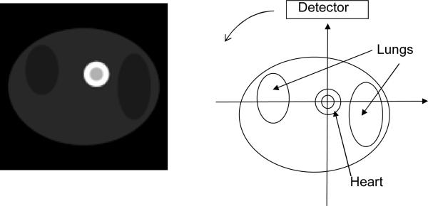
Computer simulations were conducted to verify the proposed algorithm with truncated emission data for kinetic parameter estimation. The computer generated torso phantom, shown in Fig. 1, consisted of a ring-shape myocardium with blood pool positioned within a uniform soft-tissue background with lungs. A two-dimensional 128×128 image matrix was used. Since an iterative reconstruction algorithm was used for image reconstruction, the results are independent of the imaging geometry. We use truncated parallel-hole collimation imaging geometry to simulate a dedicated cardiac system with limited FOV. The 1D detector consisted of 128 detection bins, and 402 projection views were uniformly distributed over 360°. The simulated data were reconstructed using 200 iterations of the well-known iterative ML-EM algorithm. The degree of truncation was then varied to investigate truncation effects. In the first case, 30 detector bins were truncated on both ends of the detector. In the second case, 35 bins were truncated on both ends. In the third case, 40 bins were truncated on both ends.

Figure 1.

Computer generated phantom (at time instant of 125 seconds) displayed from minimal image pixel value 0 to maximal image pixel value 0.96. The phantom consisted of a ring-shape myocardium with central blood pool, positioned in a uniform soft-tissue background with both lungs present in the image slice.

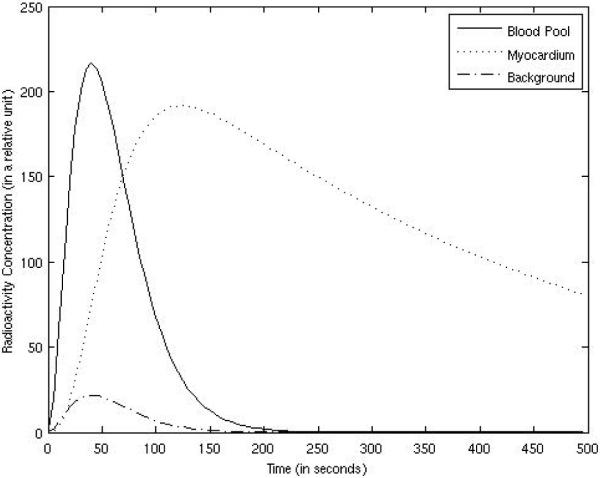
The simulated radioactivity concentration vs. time curves for the myocardium, blood pool, and the background tissues are plotted in Fig. 2. The concentration in the lungs was half of that in the background tissues. The wash-in and wash-out rates were set to K₁ = 0.015 per 5 seconds and k₂ = 0.0025 per 5 seconds, respectively. The myocardium time-activity concentration curve was calculated according to (7) with parameter f_v = 0, where the blood pool activity was arbitrarily chosen as

$$B\left(t\right)=0.005\cdot t^2{e}^{-\gamma t},t\ge 0,\text{and}\gamma =0.05\text{per}5\text{seconds}.$$ (32)

The background tissue concentration was set to 0.1B(t), and the concentration in the lungs was set to 0.05B(t). According to (7), the concentration in the myocardium is described by:

$$C\left(t\right)=0.005\cdot \frac{K_1}{{(k_2-\gamma )}^3}\{e^{-\gamma t}[{(k_2-\gamma )}^2{t}^2-2(k_2-\gamma )t+2]-2e^{-k_{2}t}\},t\ge 0,$$ (33)

where the vascular fraction f_v was set to zero for this simulation.

Figure 2.

The radioactivity concentrations in organs are functions of time.

The data sampling interval in dynamic phantom simulations was Δt = 5 seconds, and 100 timeframes were used. Thus, 100 images were reconstructed for each dynamic study. A 100-point cardiac time-activity curve and a 100-point blood-pool time-activity curve were used to estimate the parameters K₁ and k₂. For noisy cardiac projection data, the total photon count for the entire dynamic study (without truncation) was approximately 11285000, which is the sum of all photons over all 100 timeframes. For noisy data computer simulations, an ensemble of 25 different Poisson realizations of projection data was generated.

3. Results

A. The FOV bias is related to the out-of-the-FOV activity

The main assumption that the truncation-caused bias is a constant was established by Maass in his 1992 paper. Strictly speaking, as reported in Maass' paper, the other organs outside the FOV cause an almost constant bias, which has very smooth low frequency components with very small amplitude of variation. In practice, the bias caused by the data truncation may be treated as a constant. This is the reason that we made this assumption in our paper. This assumption is true even if the out-of-FOV activity has more structure. Figure 3 shows the difference image between a reconstruction without data truncation and a reconstruction with 30 bins data truncation on both ends of the detector at time instant of 125 seconds. It can be seen that inside the FOV the difference image is almost constant.

Figure 3.

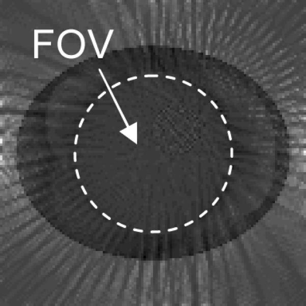
The difference image between a reconstruction without data truncation and a reconstruction with 30 bins data truncation on both ends of the detector at time instant of 125 seconds. The FOV is almost constant in this difference image. This image is displayed from a range of [−0.0238, 0.0657], which is a reduced gray scale window in order to see the small variation in the FOV.

Our empirical experience shows that the FOV bias in the iterative ML-EM reconstruction depends on the activity outside the FOV. More severe truncation results in a larger bias. In our computer simulations, the activities outside the FOV are proportional to the background activity concentration. Since the background activity is a function of time in a dynamic study, so is the bias. For the three truncation situations, the bias vs. time curves were plotted against the background concentration curves (with different scaling factors) in Figs. 4, 5, and 6. The FOVs are shown in the images in Tables 1 and 2. The bias was almost constant across the entire FOV, and was calculated over the myocardium and over the background tissue with FOV as well. As indicated by Figs. 4, 5, and 6, the bias was very small and closely followed the trend of the background concentration. In fig. 4–6, the scaling factors 0.125, 0.165, and 0.285 are estimated values. The bias was approximately 1/8 ~ 1/3.5 of the background tissue value, or 1/80 ~ 1/35 of the myocardium value.

Figure 4.

FOV bias function for the case with 30 bins being truncated on both ends of the detector is compared with 0.125 times the background concentration function.

Figure 5.

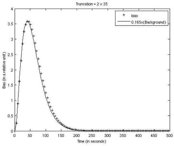
FOV bias function for the case with 35 bins being truncated on both ends of the detector is compared with 0.165 times the background concentration function.

Figure 6.

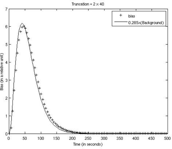
FOV bias function for the case with 40 bins being truncated on both ends of the detector is compared with 0.285 times the background concentration function.

Table 1.

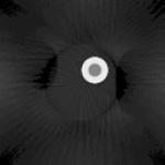
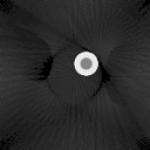
Noiseless Computer Simulation Results, in which the images are displayed in the range of [0, 63.8]. The simulations were performed with K₁= 0.015 and k₂= 0.0025 per 5 seconds

Data Truncation Situation	No truncation	30 bins are truncated on both ends of the detector	35 bins are truncated on both ends of the detector	40 bins are truncated on both ends of the detector
Summed image over reconstructions at 100 time instances
Estimated k2	0.00257	0.00256	0.00256	0.00253
Estimated K1	0.01547	0.01544	0.01541	0.01529

Table 2.

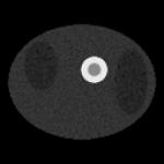
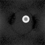
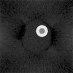
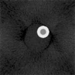
Noisy Computer Simulation Results (using s₁ = 0.0025, s₂ = 0.00005), in which the images are displayed in the range of [0, 63.8]. The simulations were performed with K₁= 0.015 and k₂= 0.0025 per 5 seconds

Data Truncation Situation	No truncation	30 bins are truncated on both ends of the detector	35 bins are truncated on both ends of the detector	40 bins are truncated on both ends of the detector
Summed image over reconstructions at 100 time instances
Estimated k2 (Average of all 25 trials)	0.00250±0.00016	0.00253±0.00017	0.00250±0.00017	0.00248±0.00016
Estimated K1 (Average of all 25 trials)	0.01496±0.00041	0.01491±0.00041	0.01488±0.00040	0.01477±0.00039

B. Verification of equation (16)

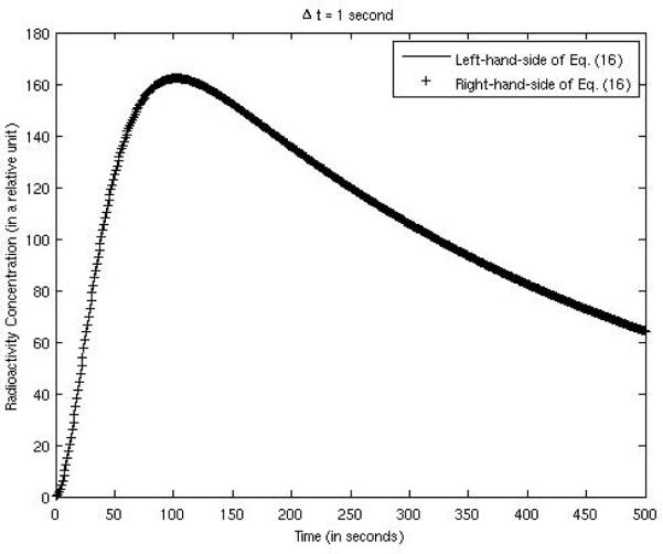
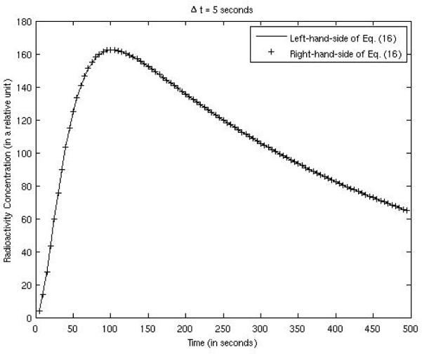
Equation (16), derived in section 2.2, is the key result of this paper; it transforms a non-linear estimation problem into a linear problem which has a closed-form solution. In the computer simulations, the bias was almost constant across the entire FOV, and was calculated over the myocardium and over the background tissue within the FOV. Both the left-hand-side and the right-hand-side of (16) are plotted in Fig. 7, compared against each other, using the example expressed by (32) and (33). The parameters were: K₁ = 0.015 per 5 seconds, k₂ = 0.0025 per 5 seconds, γ = 0.05 per 5 seconds, g = 0.2, and sampling time Δt = 1 second. The two curves matched well. When the sampling time interval was larger, e.g. Δt = 5 seconds, the two curves also matched well as shown in Fig. 8.

Figure 7.

Verification of Eq. (16) with a sampling time interval of 1 second.

Figure 8.

Verification of Eq. (16) with a sampling time interval of 5 seconds.

C. The estimation of kinetic parameters K₁ and k₂

The results of kinetic parameter estimation for a one-compartment model from noiseless computer simulations in the no data truncation situation and three different data truncation situations are summarized in Table 1, where the minimal image value is 0 and the maximum image value is 63.8. The true values for K₁ and k₂ were 0.015 and 0.0025 per 5 seconds, respectively. One hundred images were reconstructed, one image for each sampling time instant. The closed-from expressions in (27)–(30) were used to obtain the results.

D. The estimation of kinetic parameters K₁ and k₂ with noise

The results of a one-compartment model kinetic parameter estimation from noisy computer simulations in no data truncation situation and three different data truncation situations are summarized in Table 2. Formula (31) was used for the estimation of kinetic parameters K₁ and k₂, where s₁ = 0.0025 and s₂ = 0.00005 were chosen experimentally so that the bias is smaller than that with s₁ = s₂ =0. We did not perform a rigorous procedure to select s₁ and s₂ optimally. We do not know yet how to estimate the values of s₁ and s₂ directly from the reconstructed images or from the data. If we set s₁ = s₂ = 0 in (31), the corresponding results are reported in Table 3. The results in Table 3 are less accurate than those in Table 2. Therefore, a more accurate noise model of the data gives more accurate results.

Table 3.

Noisy Computer Simulation Results (using s₁ = s₂ = 0). The simulations were performed with K₁= 0.015 and k₂= 0.0025 per 5 seconds

Data Truncation Situation	No truncation	30 bins are truncated on both ends of the detector	35 bins are truncated on both ends of the detector	40 bins are truncated on both ends of the detector
Estimated k2 (Average of all 25 trials)	0.00309±0.00013	0.00307±0.00013	0.00306±0.00013	0.00302±0.00013
Estimated K1 (Average of all 25 trials)	0.01540±0.00033	0.01538±0.00034	0.01536±0.00036	0.01524±0.00033

The images shown in Table 2 do not look very noisy, because they are the summed images. The individual images (not shown) are much noisier. The computer simulation setup and image reconstruction method were the same as those in noiseless cases as in section 3.3 above, except that Poisson noise was added to the projection data.

In the noisy data computer simulations, 25 realizations of Poisson noise were generated. A significant feature of our method is that the estimated kinetic parameters were insensitive to data truncation, even though the ROI bias varies dramatically with the degree of truncation as shown in Figs. 4–6. In Tables 1, 2 and 3, the results in each row were almost the same.

4. Conclusions

This paper demonstrates that an accurate estimation of the kinetic parameters can be obtained from truncated emission projection data when certain conditions are met. Closed-form expressions for the kinetic parameters were derived and provided. The key result, shown in equation (16), describes a system of linear equations where the unknowns can be found by inverting a 3×3 matrix. equation (16) is a discrete time expression, and it holds well even for a relative large time sampling interval Δt. Our closed-form solution was inspired by earlier work (Zeng et al 1995) which first proposed to use closed-form solutions to solve compartmental modeling problems; most previous work in the area of compartmental modeling has used iterative optimization procedures. Not long ago, Murase (2004) suggested a linear least-squares solution to compartmental modeling problems; however, their linear system is much larger than our 3×3 linear system.

The proposed method first extracts time-activity curves from the ROI of the dynamic images, where the dynamic images are reconstructed via an iterative algorithm. There are many factors affecting the accuracy of the estimated parameters, including statistical noise. Our method could be improved by incorporating a better noise model into (20) and (31). The results presented in Tables 2 and 3 demonstrate that the residual error of the proposed method was independent of the degree of data truncation.

Using truncated projection data to reconstruct an image results in a biased FOV region if the image is reconstructed by an iterative algorithm. The amount of bias is roughly proportion to the truncated radioactivity outside the FOV. If the heart is entirely within the FOV and the liver is not in the image slice, the bias is determined by the background soft-tissue activity. Under the assumption that the background activity is proportional to the blood pool activity, the bias is a function of the blood pool activity. Our method is based on these assumptions.

If the liver is outside the FOV but within the image slice of interest, the bias will also depend on the liver activity, which is unknown. Then our method does not apply. A more complex FOV bias model should consider the liver time-activity model, and this topic is left for future investigation. The proposed method requires the knowledge of all models of organs that are outside the FOV but in some of the projection views. If we know the model of the background tissues and we can find a transaxial slice that does not contain the liver, either the parallel-hole or fan-beam imaging systems will work. If a cone-beam or pin-hole imaging system is used and the liver is in some of the projection views, the liver will contribute to the FOV bias and the proposed method will not work. For the purpose of simplicity, our method is presented using a single compartment model. As long as the background activity can be modeled, our method should apply regardless the number of compartments in the model. Finally, we point out that our method is able to estimate kinetic parameters such as K₁ and k₂, but cannot estimate the FOV bias in the reconstructed images because the estimation of g is influenced by both factors f_v and α as indicated by (9).

References

- Barrett HH, Wilson DW, Tsui BMW. Noise properties of the EM algorithm: I. Theory. Phys Med Biol. 1994;39:833–846. doi: 10.1088/0031-9155/39/5/004. [DOI] [PubMed] [Google Scholar]
- Blomqvist G. On the construction of functional maps in positron emission tomography. J Cereb Blood Flow Metab. 1984;4:629–632. doi: 10.1038/jcbfm.1984.89. [DOI] [PubMed] [Google Scholar]
- Blomqvist G, Pauli S, Farde L, Eriksson L, Persson A, Halldin C. Maps of receptor binding parameters in the human brain: a kinetic analysis of PET measurements. Eur J Nucl Med. 1990;16:257–265. doi: 10.1007/BF00842777. [DOI] [PubMed] [Google Scholar]
- Carson RE. Parameter estimation in positron emission tomography. In: Phelps ME, Mazziotta J, Schelbert H, editors. Positron Emission Tomography and Autoradiography: Principles and Applications for the Brain and Heart. Raven Press; New York: 1986. pp. 347–390. [Google Scholar]
- Chen C-T. Linear System Theory and Design. Holt, Rinehart and Winston, Inc.; New York, NY: 1984. [Google Scholar]
- Defrise M, Noo F, Clackdoyle R, Kudo H. Truncated Hilbert transform and image reconstruction from limited tomographic data. Inverse Problem. 2006;22:1073–1053. [Google Scholar]
- Feng D, Huang SC, Wang X. Models for computer simulation studies of input functions for tracer kinetic modeling with positron emission tomography. Int J Biomed Comput. 1993;32:95–110. doi: 10.1016/0020-7101(93)90049-c. [DOI] [PubMed] [Google Scholar]
- Forniconi AR. Least squares algorithm for region-of-interest evaluation in emission tomography. IEEE Trans Med Imaging. 1993;12:90–100. doi: 10.1109/42.222672. [DOI] [PubMed] [Google Scholar]
- Gullberg GT, Reutter BW, Sitek A, Maltz J, Budinger TF. Dynamic single photon emission computed tomography – Basic principles and cardiac applications. Phys Med Biol. 2010;55:R111–R191. doi: 10.1088/0031-9155/55/20/R01. [DOI] [PMC free article] [PubMed] [Google Scholar]
- Huang Q, Boutchko R, Hasegawa BH, Budinger TF, Gullberg GT. Computer evaluation of a novel multipinhole SPECT system for cardiac imaging. Conference Record of the 2008 IEEE Nuclear Science Symposium and Medical Imaging Conference; Dresden, Germany. Oct. 19 – 25, 2008.2008. pp. 4025–4027. [Google Scholar]
- Huang Q, Boutchko R, Reutter BW, Gullberg GT. Dynamic imaging with a novel dedicated cardiac SPECT system. J Nucl Med. 2009;50(Supp2):137P. [Google Scholar]
- Huesman RH, Mazoyer BM. Kinetic data analysis with a noisy input function. Phys Med Biol. 1987;32:1569–1579. doi: 10.1088/0031-9155/32/12/004. [DOI] [PubMed] [Google Scholar]
- Iida H, Eberl S. Quantitative assessment of regional myocardial blood flow with thallium-201 and SPECT. J Nucl Card. 1998;5:313–331. doi: 10.1016/s1071-3581(98)90133-7. [DOI] [PubMed] [Google Scholar]
- Kudo H, Courdurier M, Noo F, Defrise M. Tiny a priori knowledge solves the interior problem in computed tomography. Phys. Med. Biol. 2008;53:2207–2231. doi: 10.1088/0031-9155/53/9/001. [DOI] [PubMed] [Google Scholar]
- Maass P. The interior Radon transform. SIAM J. Appl. Math. 1992;52:710–724. [Google Scholar]
- Murase K. Efficient method for calculating kinetic parameters using T1-weighted dynamic contrast-enhanced magnetic resonance imaging. Mag. Res, Med. 2004;51:858–862. doi: 10.1002/mrm.20022. [DOI] [PubMed] [Google Scholar]
- Reske SN, Sauer W, Machulla HJ, et al. 15(p-[I-123]Iodophenyl) pentadecanoic acid as tracer of lipid metabolism: comparison with [I-14C] palmitic acid in murine tissues. J Nucl Med. 1984;25:1335–1342. [PubMed] [Google Scholar]
- Sokoloff L, Reivich M, Kennedy C, et al. The [14C]deoxyglucose method for the measurement of local cerebral glucose utilization: theory, procedure and normal values in the conscious and anesthetized albino rat. J Neurochem. 1977;28:897–916. doi: 10.1111/j.1471-4159.1977.tb10649.x. [DOI] [PubMed] [Google Scholar]
- Wilson DW, Tsui BMW, Barrett HH. Noise properties of the EM algorithm: II. Monte Carlo simulations. Phys Med Biol. 1994;39:847–871. doi: 10.1088/0031-9155/39/5/005. [DOI] [PubMed] [Google Scholar]
- Ye Y, Yu H, Wang G. A general local reconstruction approach based on a truncated Hilbert transform. Int. J. Biomed. Imaging. 2007:63634. doi: 10.1155/2007/63634. [DOI] [PMC free article] [PubMed] [Google Scholar]
- Zeng GL, Gullberg GT. Single photon emission local tomography (SPELT). 1996 IEEE Nuclear Science Symposium Conference Record; Nov. 2 – 9, 1996; California: Anaheim; 1996. pp. 1628–1632. [Google Scholar]
- Zeng GL, Gullberg GT. Exact emission SPECT reconstruction with truncated transmission data. Phys. Med. Biol. 2009a;54:3329–3340. doi: 10.1088/0031-9155/54/11/004. [DOI] [PMC free article] [PubMed] [Google Scholar]
- Zeng GL, Gullberg GT. Exact iterative reconstruction for the interior problem. Phys. Med. Biol. 2009b;54:5805–5814. doi: 10.1088/0031-9155/54/19/009. [DOI] [PMC free article] [PubMed] [Google Scholar]
- Zeng GL, Gullberg GT. SPECT region of interest reconstruction with truncated transmission and emission data. Med Phys. 2010;37:4627–4633. doi: 10.1118/1.3471376. [DOI] [PMC free article] [PubMed] [Google Scholar]
- Zeng GL, Gullberg GT, Huesman RH. Using linear time-invariant system theory to estimate kinetic parameters directly from projection measurements. IEEE Trans. Nucl. Sci. 1995;42:2339–2346. [Google Scholar]