Quiescence: a mechanism for escaping the effects of drug on cell populations

Abstract

We point out that a simple and generic strategy in order to lower the risk for extinction consists in developing a dormant stage in which the organism is unable to multiply but may die. The dormant organism is protected against the poisonous environment. The result is to increase the survival probability of the entire population by introducing a type of zero reproductive fitness. This is possible, because the reservoir of dormant individuals act as a buffer that can cushion fatal fluctuations in the number of births and deaths, which without the dormant population would have driven the entire population to extinction.

1. Introduction

Drug resistance is a very serious problem not least for chemotherapeutic treatment of cancer, and it is very important to understand, as far as possible, the ways to countermeasure drug resistance in a number of biomedical contexts. In order to unravel the possible mechanisms responsible for this phenomena, Iwasa and co-workers [1,2] developed a prominent theoretical model of the evolutionary dynamics of escape. They base their approach on the assumption that n point mutations in some crucial parts of the genome are necessary for escape. They further assumed that the different mutants can be described by binary strings (with entries of +1 or −1) of length n. There are 2ⁿ − 1 such mutants. It is assumed that treatment reduces the proliferation ratios of sensitive mutants, R < 1; whereas resistant mutants are such that R > 1. The corresponding evolutionary dynamics is modelled in terms of Galton–Watson multi-type branching process (GWMBP; [3]), where at each generation each individual of each type has a given (in general, mutant-dependent) probability of mutating and producing offspring belonging to a different type. The problem is to calculate the probability that a resistant mutant is reached within a population of size N. The model proposed by Iwasa and co-workers has been analysed in more detail by Serra [4] and Serra & Haccou [5]. While this approach is both biologically and mathematically sound, we believe that the efficiency with which evolutionary escape allows organisms to avoid extinction, when attacked by lethal drug, can be understood in a more simple way as a consequence of a dormant phase. To assess the generic importance of dormancy as an escape strategy, we develop a very simple model framework, in which we only focus on the most essential aspects of population and evolution dynamics.

Here, we show that the existence of a dormant phase can be crucial for a population to escape extinction. We consider the following simplified scenario. We study the survival probability of a population of organisms that can exist in the form of three different types (figure 1). The types differ in their response to the presence of a drug. Types (1) and (2) have similar reproduction and death rates when no drug is present. However, the drug is supposed to be lethal to type (2) but neutral to type (1). We are interested in how the existence of a dormant mode, type (3), affects the survival probability of the entire population. The dormant type can neither reproduce, nor is it susceptible to the drug. However type (3) can die and it can undergo a transformation back to type (1). To understand the effect of the dormant type, we consider different realizations (indicated in figure 1) of the possible flow between the three different types.

Figure 1.

Schematic of the population dynamics considered in this paper. The arrows between the different types of individuals represent the possible population flows between them. The arrows pointing to the types themselves represent proliferation. The other arrows stand for death of each type of individuals. The thickness of the arrows stand for the relative magnitude of each of the flows or processes. (a) Model A; (b) model B; (c) model C.

Our model is relevant to a number of biological cases, in particular to entities such as cancer cells, which have been observed to evolve resistance to therapy: treatments impose a selective pressure that eliminates the lesser fit strands of the corresponding populations but also drives an evolutionary process, whereby better adapted individuals, i.e. individuals immune to the effects of the corresponding drug, eventually take over. Further rationale for our model is provided by the response of tumour cells to hypoxia (i.e. oxygen starvation). It is a well-known fact that hypoxia induces arrest of the cell cycle [6,7]. This means that the rate at which cells replicate under hypoxia is drastically reduced, as hypoxia downregulates the activity of the pathway regulating the progression through the cell cycle [6]. Moreover, another well-understood fact about cell survival/death regulation is that there exists cross-talk between the pathways regulating cell death and cell division [8–10]. This means that, in normal circumstances, the downregulation of the cell cycle machinery implies the downregulation of the apoptotic (programmed cell death) machinery. It can be argued that such cross-talk is disrupted in cancer cells, and that cancer cells are such that cell death regulatory pathways are downregulated. Therefore, under hypoxic conditions, cancer cells undergo a drastic reduction of their division and death rates.

The study of the influence of hypoxic cancer cells fits rather well within the original remit in which the dynamics of evolutionary escape was put forward, as hypoxic cells are known to play a major role in the resistance to chemotherapy and radiotherapy in tumours [11]. To study the influence of such a subpopulation on the global dynamics of the total population, we model it as a dormant or quiescent population with negligible proliferation rate and small death rate.

Previous works have analysed some of the effects of quiescent cells on tumour growth (e.g. [12,13]). All these previous studies hint on the role of quiescence cells in the dynamics of tumour growth and its role in resistance to tumour growth, but the issue of the evolutionary dynamics involved is not directly addressed.

We now turn to the study of the survival probability. We disentangle the interplay between drug susceptibility, type (2) and dormancy, type (3), by analysing three different versions of the population dynamics, all of which are depicted in figure 1 and formulated as the following three models.

Model A. This is the ‘normal’ situation, where no drug is present. Types (1) and (2) are essentially equivalent, except that when type (1) reproduces, it may undergo a ‘mutation’ and end up as type (3). When type (2) reproduces it may mutate and become type (1).

Model B. This is the situation in the presence of the drug. The death rate of type (2) is now significantly bigger than the death rates of types (1) and (3). Moreover, the drug makes type (2) unable to reproduce and therefore the flow from type (2) to type (1) is absent.

Below, we will find that the dormant stage increases the survival probability of the population in the presence of the drug. To emphasize that the increased ability of the population to escape extinction is in fact caused by the presence of a dormant stage, we also consider an extreme version of the dynamics in which type (1) is unable to die.

Model C. This version of the the dynamics is equivalent to model B except that type (1) now is assumed not to be able to die directly, but has to flow through either type (2) or type (3) to do so. We then demonstrate that even in this extreme situation does the availability of the dormant stage enhances the population's chance for avoiding extinction.

We notice that the different types (1), (2) and (3) can be thought in epidemiological terms as susceptible, infected and immune. The version of the dynamics defined as model B can be thought to represent an age-structured population. Type (3) is then juveniles, type (1) are mature reproduction active individuals and type (2) are individuals in the post-reproductive stage.

An economical and precise way to present the dynamics is in terms of the generator functions for the corresponding Galton–Watson multi-type branching process. We include these generator functions in the tables in the appendix A. Within the theory of multi-type branching process, the condition for eventual non-extinction is given in terms of the spectral radius, ρ, of the matrix A = (a_ij), whose entries are the expected values of the number of offspring of type j produced of an individual of type i. If ρ > 1, there is a finite probability of N(t → ∞) > 0. The quantities a_ij are calculated in terms of the corresponding generating functions (table 2): A_ij = ∂_jG_i|_x̄=1. From these standard arguments of the theory of multi-type branching process, which carry on in a straightforward manner when size-dependence is taken into account [14], we can establish from tables 1 and 2 in appendix A, that the condition for asymptotic survival, that is for P[N(t → ∞) > 0] > 0, is

1.1

i.e. r₁₂ < 1/2. Otherwise, the probability of eventual extinction is 1. Now, consider the presence of a third type (type (3)) within the population, namely, quiescent individuals. These individuals are not allowed to proliferate but are resilient to the environment and can survive under hostile conditions, hence we assume that their death rate ε ≪ 1. In addition, quiescent cells are assumed to be able to revert back to type (1) at a given rate, which depends on the availability of resources. The issue we intend to analyse is whether the introduction of a quiescent subpopulation helps to escape from the whole population being extinct. More precisely, the question we aim to address is: assume r₁₂ ≥ 1/2, is it possible for a population whose dynamics is described in model B and table 2 to elude eventual extinction? specifically, this scenario has been considered within the context of modelling of tumour growth, in particular, in the response of cancer cells to hypoxia (low levels of oxygen; [12]). Cancer cells appear to become quiescent in response to hypoxia, which is thought to give them an advantage in their competition with their normal counterparts as well as resistance to radiotherapy and chemotherapy [15].

Table 2.

Model B. Generating functions of the probabilities of the number of offspring for individuals of type (1), i.e. well adapted to harsh conditions, G₁(x̄), type (2), i.e. those for which the environment is lethal, G₂(x̄) and type (3), i.e. quiescent individuals, G₃(x̄). The parameter μ is the carrying capacity, which accounts for the limitation in resources, α is a measure of the remnant resilience of individuals of type (2) to the environment, and ε is the death rate (probability of death per individual per generation) of the quiescent cells. The quantity r_1j with j = 1,2 can be interpreted as the mutation rate of individuals of type (1) into individuals of type j. The quantity r₃₁ is the probability per quiescent individual per generation of a type (3) individual to revert to type (1).

population 1	G1 (x̄) = 1 − e−μN + e−μNr12x22 + e−μNr13x32 + e−μN(1 − r12 − r13)x12
population 2	G2 (x̄) = α+ (1 − α)x2
population 3	G3 (x̄) = ε+ r31 e−μNx1 + (1 − ε− r31 e−μN)x3

Table 1.

Model A. Generating functions of the probabilities of the number of offspring for individuals belonging to our population earlier to the introduction of a hostile agent. In this situation, both types (1) and (2) individuals are well adapted and can proliferate subject to the restrictions imposed by the carrying capacity. Type (3) correspond to quiescent individuals. The new parameters introduced here are r₂₁, i.e. the mutation probability of type (2) into type 1, the probability of a type (2) individual to enter quiescence, r₂₃ and the probability of a quiescent individual to revert to type (2). The rest of the parameters have the same physical meaning as in table 2.

population 1	G1 (x̄) = 1− e−μN + e−μNr12x22 + e−μNr13x32 + e−μN (1 − r12 − r13)x12
population 2	G2 (x̄) = 1 − e−μN + e−μNr21x22 + e−μNr23x32 + e−μN (1 − r21 − r13)x12
population 3	G3 (x̄) = ε+ r31e−μNx1 + r32 e−μNx2 + (1 − ε− (r31 + r32)e−μN)x3

We now present the results of simulations of the survival probability for the three different scenarios represented by models A, B and C.

2. Simulation results

Numerical simulations of the underlying multi-type branching process (see appendix A for details) confirm that, in fact, the presence of a quiescent population as a mechanism to escape from harsh conditions is indeed feasible. Figure 2 shows how the survival probability depends on the probability of an individual of type (1) to become quiescent, r₁₃. We can see that as r₁₃ decreases, the threshold for survival in terms of r₃₁, i.e. the probability of a quiescent individual to revert to type (1), moves towards smaller values of the parameter r₃₁. This means that, following a decrease in the flux of individuals from the type (1) population to type (3), survival is only possible by reducing the inverse flux. This observation reveals that the mechanism by which quiescence helps escape is by acting as a reservoir, where part of the population can be safely ‘stored’. If the flux from type (3) back to type (1) is too big, it effectively increases the flux from type (1) to type (2), thus increasing lethality. This behaviour, however, is sensitive to the decay rate of type (3) individuals, ε: as this parameter increases, the survival probability decreases (figure 4). This means that the death rate of quiescent individuals being small is an instrumental factor for quiescence-induced escape from harsh environments.

Figure 2.

Simulation results for r₁₂ = 0.5. Black circles correspond to r₁₃ = 0.5 and black squares to r₁₃ = 0.25. Other parameter values: μ = 0.001, ε = 10⁻⁵ and α = 1.

Figure 4.

Simulation results for r₁₃ = 0.5 and r₁₂ = 0.5, and black diamonds to r₁₂ = 0.5. Black circles correspond to r₃₁ = 0.05 and black squares r₃₁ = 0.1. Other parameter values: μ = 0.001 and α = 1.

Figure 3 shows that as r₁₂ increases further into the regime, where equation (1.1) predicts sure extinction of the type (2) population, survival is only possible by decreasing r₃₁, i.e. by increasing the average time individuals spent in the quiescent state.

Figure 3.

Simulation results for r₁₃ = 0.5. Black circles correspond to r₁₂ = 0.5, black squares to r₁₂ = 0.525 and grey diamonds to r₁₂ = 0.55. Other parameter values: μ = 0.001, ε = 10⁻⁵ and α = 1.

To test this scenario further, we perform simulations in which the following situation is considered. First, we let a population whose dynamics is given by model A, evolve for some time in an environment free of the hostile agent. In this environment, individuals of both types (1) and (2) can thrive. The dynamics in an environment free of any hostile agent is described in terms of the generating functions shown in table 1. The introduction of the hostile agent is described by changing the dynamics of the population to the one described by model B (figure 1 and table 2), which is essentially the same as model A (table 1) but with type (2) individuals doomed to perish. We further assume that the hostile agent is active only for a given period of time, after which its detrimental effect on type (2) organisms ceases and the dynamics of the population reverts to model A (according to table 1). Parameter values are chosen so the dynamics of the agent-free population is super-critical (i.e. the corresponding survival probability is bigger than zero). After the hostile agent has been removed, we calculate the probability that the population survives both with and without quiescence. This scenario is highly relevant to evolutionary escape from drugs, which have a finite lifespan. This particular escape problem was considered [1].

The corresponding results are shown in figures 5 and 6. Figure 6 shows the survival probability, P[N > 0], as a function of r₁₃ and, indeed, we observe that when quiescent individuals are not considered, i.e. r₁₃ = 0, the probability of surviving after the end of the activity period of the hostile agent is null. As r₁₃ increases, so does the corresponding survival probability, thus further confirming that quiescence is a feasible mechanism to help biological populations to escape harsh environmental conditions. Moreover, figure 5, which shows particular realizations of the process with (figure 5b), and without (2a) quiescence, also helps in understanding more about the mechanism, whereby quiescence allows escape: as can be seen in figure 5b, during the period of activity of the hostile agent most of the population is actually quiescent with a little proportion of the population in types (1) and (2). This means that quiescence mediates survival by acting as a reservoir or buffer.

Figure 5.

Simulation results showing one realization of the population dynamics of the reaction to the (transient) application of a therapeutic agent. We can see that in plot (a), which corresponds to a population with no quiescent state, the population upon application of the drug. On the contrary, a population with quiescence is able to survive to the period over which the drug is active, and recovering once the effect of the drug has worn off (b). Black lines correspond to the total population, red lines to individuals of type (1), green lines to individuals of type (2) and blue lines to quiescent (type (3)) individuals. Parameter values: r₁₂ = r₂₁ = 0.5, r₁₃ = r₃₁ = 0 for the upper panel and r₁₃ = r₃₁ = 0.25 for the lower panel, r₃₁ = 0.05, μ = 0.001, ε = 10⁻⁵ and α = 1. (a) r₁₃ = 0; r₁₃≠0.

Figure 6.

Simulation results showing the survival probability, P(N > 0), for the population dynamics of the reaction to the (transient) application of a therapeutic agent as a function of the parameter r₁₃, i.e. the parameter controlling the flux of population between types (1) and (3). Parameter values: r₁₂ = r₂₁ = 0.5, r₃₁ = 0.05, μ = 0.001, ε = 10⁻⁵ and α = 1.

3. An alternative model

Although the results discussed until here provide compelling evidence in favour of hypothesis that the presence of quiescence can induce escape without the need of an increase in the reproductive fitness of any particular type of organism, some doubt could be cast on our argument so far. One might feel inclined to argue that our model still relies on a multi-type population, where one type (type (1)) is effectively more fit than the others. To address this possibility, we consider model C in figure 1. This version is closely related to the current discussion concerning the response of cancer cells to oxygen starvation. This model is also formulated in terms of a GWMBP and characterized in terms of the generating functions given in table 3. Its rationale is as follows. Let us assume that a population of cells is divided into two types: those in which the pathways regulating cell division are activated (type (1)) and those in which the active pathways are those regulating apoptosis, i.e. cell death (type (2)). Type (1) cells can either proliferate, or stay as they are, or suffering activation of the apoptotic pathways, thus becoming type (2) cells. The flux of population between types (1) and (2) is controlled by the parameter r₁₂. Type (2) cells are those marked for cell death, but the model provides for their staying within the population for a while (not dying immediately), but they cannot proliferate. Type (3) cells are, as in the previous model, quiescent cells. In this context, the introduction of a hostile agent (drug, removal of oxygen, etc.) corresponds simply to increasing the value of r₁₂.

Table 3.

Generating functions corresponding to model C (see main text for details). Types 1 and 2 correspond to the proliferative and apoptotic phenotypes, respectively. Type 3 corresponds to the quiescence population.

population 1	G1 (s̄) = (1 − e−μN)x + e−μNr12x22 + e−μNr13x32 + e−μN (1 − r12 − r13)x12
population 2	G2 (s̄) = α+ (1 − α)x2
population 3	G3 (s̄) = ε+ r31e−μNx1 + (1 − ε− r31e−μN)x3

In the absence of quiescence, standard arguments reveal that extinction with probability 1 occurs when r₁₂ ≥ 1/2. The question is once again whether quiescence can rescue the population from extinction under such conditions. Figure 7 shows that this is indeed the case, provided that the flux out of the quiescent state back into type (1) does not exceed a critical value. These results are completely analogous to those obtained for the previous model.

Figure 7.

Simulation results for model C with r₁₂ = 0.51. Black circles correspond to r₁₃ = 0.45 and black squares to r₁₃ = 0.25. Other parameter values: μ = 0.001, ε = 10⁻⁵ and α = 1.

4. Invasion dynamics

We now discuss under which conditions a small proportion of individuals, y, which can undergo quiescence, modelled by models A and B depending on whether a drug is present or not, respectively, and with r₁₃ ≠ 0, can take over a population of fully growing individuals, i.e. a population modelled by models A and B with r₁₃ = 0. In particular, we will analyse the corresponding invasion probability, P_F(y), by direct simulation of the population dynamics and by using the analytical approximation provided by the so-called evolutionary formalism [16–19], which allows a more thorough exploration of the behaviour of the invasion probability as a function of the model parameters.

The problem we address here relates to whether a small population of mutants can take over an incumbent population. Demetrius and co-workers [17,19] have developed a formalism based on the application of ideas from ergodic theory to evolutionary problems [16] and the diffusion approximation [20]. This formalism allows us to estimate the fixation probability of a mutant population in the presence of an incumbent species. Here, we generalize this formalism to apply it to the problem of whether a genetic inactivation generating new phenotypes can invade the incumbent population.

The starting point of this formalism is the following fundamental equation:

4.1

where r = log(Λ₀) is the growth rate (or Malthusian parameter), with Λ₀ being the dominant eigenvalue of A, whereas H and F are the entropy and the proliferative potential, defined as:

4.2

where is defined as:

4.3

with , and π is the stationary distribution associated to , with given by . Equations (4.1–4.3) are derived from a variational principle [16], namely

4.4

where ν is a Markov measure, H_ν = −∑_j=1ⁿν(A_j) log ν(A_j) and γ = loga_x0x1, where A_j, j = 1, … , n is a partition of the phase space of the system and a_x0x1 is the transition probability between two states of the system, x₀ and x₁. The solution to this variational problem produces equations (4.1–4.3) [16,21].

According to Demetrius et al. [19], the diffusion approximation yields the following equation for the fixation or invasion probability as a function of the initial concentration of mutants, y is given by:

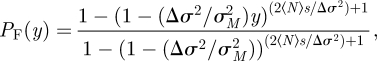4.5

where the total population N is assumed to be constant and s is defined by:

4.6

where Δr ≡ r_q − r, Δσ² = σ_q² − σ², with r_q(r) is the growth rate of the quiescence (normal) population, and σ_q²(σ²) is the variance of the quiescent (normal) population, 〈N〉 is the average stationary population.

The demographic parameters (i.e. r, σ², r_q, and σ_q²) can be estimated from the evolutionary formalism (see [18,19]). The growth rates are given by r = log λ₀, where λ₀ is the dominant eigenvalue of the of the matrix A = (a_ij) = (∂_jG_i(x̄)|_x̄=1). In [19], it is shown that the parameter σ² can be obtained by slightly perturbing the parameters that determine the dynamics of the system, i.e. the mean-field dynamics being given by A(δ) = (a_ij^1+δ), and then doing an expansion for small δ. Accordingly, σ² is given by:

4.7

Hence, in the linear approximation with H(δ) given by H(δ) = H + δH_δ, we have that σ²(γ) = −Hδ, which is given by:

4.8

where π_i(δ) = π_i + δπ_i^(δ) and p_ij(δ) = p_ij + δp_ij^(δ) are the corresponding linear approximations to π and P = (p_ij), when we take A(δ) = (a_ij^1+δ) δ ≪1. The details of how these quantities are actually calculated is given in appendix A of Alarcón & Jensen [18].

In order to show that this formalism can be used to analyse the invasion of a population possessing a dormant type, we have done simulations where one population, which is sensitive to the drug, competes with two different population: one capable of undergoing quiescence and another one which is unable to enter such state. We compare the numerics with the analytical results obtained from equation (4.5) in figure 8. Both analytical and numerical results show that whereas in the former case the quiescent population takes over the sensitive population almost surely, in the latter case it is unlikely that the non-resident population takes over the resident one. It is worth remarking that the good agreement between simulations and analytical result seen in figure 8 implies that the evolutionary formalism developed by Demetrius and co-workers [17,19] is able to make the invasion problem considered here analytically tractable.

Figure 8.

Fixation probability for the competition between two populations in the presence of drug. Squares correspond to the competition with a population capable of undergoing quiescence, whereas circles correspond to the competition with a population that cannot undergo quiescence. Solid line corresponds to the analytical expression of P_F(y) for the latter case.

5. Summary and discussion

We have shown that quiescence is a feasible mechanism for biological populations to escape hostile environments. This mechanism is expected to be very relevant to the important issue concerning population dynamics of cancer cells and the competition mechanisms between cancer cells and their normal counterparts. In particular, our model addresses issues related to the response of cancer cells to oxygen starvation [11,15]. The mechanism involved in quiescence-dependent escape is in essence simple: it provides a buffer for the population to be safe from the hostile environment. That is, in cases where the population would go extinct owing to a fluctuation in the birth and death events, the reservoir in the quiescence buffer population can bring the population back from the brink of extinction. The efficiency of this mechanism for escape is sensitive to the entry and exit rates to and from the quiescent state, respectively.

The main difference between our mechanism for escape and the one proposed in Iwasa et al. [1,2] is the following. Iwasa and co-workers propose a mechanism based on random search of the state of types of individuals for one that is fitter than the others in the presence of a given selection pressure (drug, etc.). In contrast, we have demonstrated here that the overall survival probability of a population may increase by introducing a dormant type. Since this type is unable to reproduce, its reproductive fitness is zero; nevertheless, the existence of this drug-resistant stage is able to improve the fitness of the entire population inasmuch as the population obtains a higher probability for survival.

The mechanism proposed here shares a number of features in common with the phenomenon of bacterial persistence [22–25]. Persistence is a form of resistance to antibiotics exhibited by bacterial colonies, where resistance is not acquired by a gene mutation that allows the bacteria to grow exponentially fast in the presence of a particular drug. Instead, as schematically shown in figure 9, killing of bacteria goes through a fast phase, where the population decreases exponentially until the killing rate slows down leaving behind a remnant of cells, which differ from the sensitive ones in that they are in a dormant state but are otherwise genetically identical to their sensitive counterparts. In fact, when the drug is removed, a colony of ‘normal’ bacteria is regrown from the persistent cells. The mechanism for persistence appears to involve a phenotypic switch [22], where cells switch from a rapidly growing, but drug-sensitive phenotype to a dormant but drug-resistant phenotype, although there has recently been the suggestion that persistence might be a social trait [24].

Figure 9.

This plot illustrates the phenomenon of persistence. After introducing a drug (typically, an antibiotic), there is an initial period of fast decay of the population followed by a crossover after which the rate of population decays is much slower. In bacterial populations such as Escherichia coli, this is thought to be owing to a phenotype switch: cells switch to a slow-growing phenotype that is more resilient to the effect of the drug than the normal phenotype. This phenomenon cannot be of genetic origin, as cells regrown from the persistent population upon removal of the drug are sensitive to it [22].

According to Balaban et al. [22], there exist two types of persister. Type I persister, according to their terminology, are only produced during the exponential growth phase and therefore their numbers are fixed at the time of inoculation and determined by the size of the inoculum. Type II persister, on the contrary, divide and grow continuously, but an order of magnitude slower than their non-persistent counterparts, and their numbers are determined by the total population numbers. The quiescence mechanism put forward here is therefore distinct from type I persister, but very similar to the behaviour exhibited by type II persister, which means that the analysis methods, in particular, the evolutionary formalism used to study the competition between subpopulations exhibiting different behaviour, can be extended to study this type of bacterial persistence.

Another issue in which our model differs from previous work on bacterial persistence is the following. We are considering different populations adopting different strategies, namely, a wild-type population that thrives in the absence of drug composed of two subpopulations: one that is capable of undergoing quiescence and another one that is not. By adopting this scenario, we can study the evolutionary dynamics of these populations and analyse which strategy is evolutionarily stable and which one is susceptible to be invaded. In that respect, our analysis goes beyond, for example, the population models proposed by Balaban et al. [22].

Within the context of the problem of how the hypoxic subpopulation affects the dynamics of the whole tumour, our model sheds further light on this issue. It is commonly thought that hypoxia increases the probability of survival of the tumour by providing a selective pressure that favours the evolution and survival of more aggressive phenotypes [11]. Our model shows that quiescence by itself is enough to increase the survival probability of the population without further increase in the phenotypic variety of the population. Obviously, the residual population provides a springboard for these evolutionary processes to ensue.

Appendix A. Simulations

In this appendix, we briefly describe the method we have used to produce our simulation results. Our simulations start with one single individual of type (1). Its offspring is determined by the probabilities of producing descendants as prescribed by the generating functions given in tables 1–3, corresponding to models A, B and C, respectively. In general, the coefficients of the Taylor expansion of G_i(x̄) = ∑_l,n,m=0 P_i;lnmx₁^l x₂ⁿ x₃^m are the probabilities per generation per individual (of type i) that a type i-individual produces l descendants of type (1), n descendants of type (2) and m descendants of type (3). In subsequent generations, we go over all the individuals in existence in the last generation and the numbers and types of their descendants within the next generation are calculated in the same way. Simulations are run over 1000 realizations of 1000 generations each. The survival probability, P[N > 0], is calculated as the ratio between the number of simulations such that N(T = 1000) > 0 and the total number of realizations.

References

- 1.Iwasa Y., Michor F., Nowak M. A. 2003. Evolutionary dynamics of escape from biomedical intervention. Proc. R. Soc. Lond. B 270, 2573–2578 10.1098/rspb.2003.2539 (doi:10.1098/rspb.2003.2539) [DOI] [PMC free article] [PubMed] [Google Scholar]
- 2.Iwasa Y., Mchor F., Nowak M. A. 2004. Evolutionary dynamics of invasion and escape. J. Theor. Biol. 226, 205–214 10.1016/j.jtbi.2003.08.014 (doi:10.1016/j.jtbi.2003.08.014) [DOI] [PubMed] [Google Scholar]
- 3.Kimmel M., Axelrod D. E. 2002. Branching processes in biology. New York, USA: Springer [Google Scholar]
- 4.Serra M. C. 2006. On the waiting time to escape. J. Appl. Prob. 43, 296–302 10.1239/jap/1143936262 (doi:10.1239/jap/1143936262) [DOI] [Google Scholar]
- 5.Serra M. C., Haccou P. 2007. Dynamics of escape mutants. Theor. Popul. Biol. 72, 167–178 10.1016/j.tpb.2007.01.005 (doi:10.1016/j.tpb.2007.01.005) [DOI] [PubMed] [Google Scholar]
- 6.Gardner L. B., Li Q., Parks M. S., Flanagan W. M., Semenza G. L., Dang C. V. 2001. Hypoxia inhibits g1/s transition through regulation of p27 expression. J. Biol. Chem. 276, 7919–7926 10.1074/jbc.M010189200 (doi:10.1074/jbc.M010189200) [DOI] [PubMed] [Google Scholar]
- 7.Alarcón T., Byrne H. M., Maini P. K. 2004. A mathematical model of the effects of hypoxia on the cell-cycle of normal and cancer cells. J. Theor. Biol. 229, 395–411 10.1016/j.jtbi.2004.04.016 (doi:10.1016/j.jtbi.2004.04.016) [DOI] [PubMed] [Google Scholar]
- 8.Nishioka W. K., Welsh R. M. 1994. Susceptibility to cytotoxic t-lymphocyte induced apoptosis is a function of the proliferative status of the target. J. Exp. Med. 179, 769–774 10.1084/jem.179.2.769 (doi:10.1084/jem.179.2.769) [DOI] [PMC free article] [PubMed] [Google Scholar]
- 9.Padmanabhan J., Park D. S., Greene L. A., Shelanski M. L. 1999. Role of cell-cycle regulatory proteins in cerebellar granule neuron apoptosis. J. Neurosci. 19, 8747–8756 [DOI] [PMC free article] [PubMed] [Google Scholar]
- 10.Alberts B., Johnson A., Lewis J., Raff M., Roberts K., Walter P. 2002. Molecular biology of the cell, 4th edn. New York, NY: Garland Publishing Inc [Google Scholar]
- 11.Bristow R. G., Hill R. P. 2008. Hypoxia, DNA repair and genetic instability. Nat. Rev. Cancer 8, 180–192 10.1038/nrc2344 (doi:10.1038/nrc2344) [DOI] [PubMed] [Google Scholar]
- 12.Alarcón T., Byrne H. M., Maini P. K. 2003. A cellular automaton model of tumour growth in an inhomogeneous environment. J. Theor. Biol. 225, 395–411 [DOI] [PubMed] [Google Scholar]
- 13.Brikci F. B., Clairanbault J., Ribba B., Perthame B. 2008. An age-and-cyclin-structured cell population model for healthy and tumoural tissues. J. Math. Biol. 57, 91–110 [DOI] [PubMed] [Google Scholar]
- 14.Jagers P. 1999. Branching processes with dependence but homogeneous growth. Ann. Appl. Prob. 9, 1160–1174 [Google Scholar]
- 15.Brown J. M., Wilson W. R. 2004. Exploiting tumour hypoxia in cancer treatment. Nat. Rev. Cancer 4, 437–447 10.1038/nrc1367 (doi:10.1038/nrc1367) [DOI] [PubMed] [Google Scholar]
- 16.Arnold L., Gundlach V. M., Demetrius L. 1994. Evolutionary formalism for products of positive random matrices. Ann. Appl. Prob. 4, 859–901 10.1214/aoap/1177004975 (doi:10.1214/aoap/1177004975) [DOI] [Google Scholar]
- 17.Demetrius L. 1997. Directionality principles in thermodynamics and evolution. Proc. Natl Acad. Sci. USA 64, 3491–3498 [DOI] [PMC free article] [PubMed] [Google Scholar]
- 18.Alarcón T., Jensen H. J. Submitted Invasion in multi-type populations: the role of robustness and fluctuations. [DOI] [PubMed] [Google Scholar]
- 19.Demetrius L., Gundlach V. M., Ochs G. 2009. Invasion exponents in biological networks. Physica A 388, 651–672 10.1016/j.physa.2008.10.048 (doi:10.1016/j.physa.2008.10.048) [DOI] [Google Scholar]
- 20.Feller W. 1951. Diffusion processes in genetics. In Proc. 2nd Berkeley Symp. on Mathematical Statistics and Probability (ed. Neiman J.), Berkeley, California, 31 July–12 August 1950. Berkeley, California: University of California [Google Scholar]
- 21.Billingsley P. 1965. Ergodic theory and information. New York: John Wiley & Sons [Google Scholar]
- 22.Balaban N. Q., Merrin J., Chait R., Kowalik L., Leibler S. 2004. Bacterial persistence as a phenotypic switch. Science 305, 1622–1625 10.1126/science.1099390 (doi:10.1126/science.1099390) [DOI] [PubMed] [Google Scholar]
- 23.Levin B. R., Rozen D. E. 2006. Non-inherited antibiotic resistance. Nat. Rev. Microbiol. 4, 556–563 10.1038/nrmicro1445 (doi:10.1038/nrmicro1445) [DOI] [PubMed] [Google Scholar]
- 24.Gardner A., West S. A., Griffin A. S. 2007. Is bacterial persistence a social trait? PLoS ONE 8, e752. [DOI] [PMC free article] [PubMed] [Google Scholar]
- 25.Lewis K. 2007. Persister cells, dormancy and infectious disease. Nat. Rev. Microbiol. 5, 48–56 10.1038/nrmicro1557 (doi:10.1038/nrmicro1557) [DOI] [PubMed] [Google Scholar]