Predicting judged similarity of natural categories from their neural representations

Abstract

We report a combined behavioral and functional magnetic resonance imaging (fMRI) study of conceptual similarity among members of a natural category (mammals). The study examined the relationship between computed pairwise similarity of neural responses to viewed mammals (e.g. bear, camel, dolphin) and subjective pairwise similarity ratings of the same set of mammals, obtained from subjects after the scanning session. In each functional region of interest (fROI), measures of neural similarity were compared to behavioral ratings. fROIs were identified as clusters of voxels that discriminated intact versus scrambled images of mammals (no information about similarity was used to define fROIs). Neural similarity was well correlated with behavioral ratings in fROIs covering the lateral occipital complex in both hemispheres (with overlap of the fusiform and inferior temporal gyri on the right side). The latter fROIs showed greater hemodynamic response to intact versus scrambled images of mammals whereas the fROIs that failed to predict similarity showed the reverse pattern. The findings provide novel evidence that information about the fine structure of natural categories is coarsely coded in regions of the ventral visual pathway. Implications for the theory of inductive inference are discussed.

Interest in the neural representation of concepts has grown out of the discovery of category-specific memory impairments (Warrington & McCarthy, 1987; Warrington & Shallice, 1984) along with the more global degradation of conceptual knowledge known as semantic dementia (Snowden, Goulding, & Neary, 1989; Warrington, 1975). Much of the ensuing research has focused on the extent to which variation across cortical areas is better characterized in category-specific or modality-specific terms. For example, Martin, Wiggs, Ungerleider, & Haxby (1996) discovered that naming both animals and tools activates ventral temporal cortex and Broca’s area, while naming only animals activated the left occipital lobe, and naming only tools activated left premotor and middle temporal cortices. (For discussion, see Caramazza & Mahon, 2003, and Martin, 2007.)

In a recent review, Tyler et al. (2003) concluded that “the most striking finding in the neuroimaging studies of category and domain specificity is that most categories activate the same neural regions with only weak and inconsistent category-specific effects.” The lack of category-specificity suggests shared substrata for diverse concepts, with the identity of a given category coded by the pattern of activation across an entire region. Most current fMRI analysis methods are not optimally suited for testing this hypothesis because they employ a univariate approach to category discrimination (based on different locations of peaks and clusters), which focuses on a region’s overall metabolic response to different categories.

The univariate strategy contrasts with recently developed analytic methods that focus on the information carried by the pattern of activation in a given region of the brain. For example, Haxby et al. (2001) and Cox and Savoy (2003) succeeded in classifying different categories of objects on the basis of response patterns provoked by those objects in ventral temporal and ventrolateral occipital cortices. Likewise, machine learning techniques have succeeded in decoding patterns of neural activity to predict orientation of viewed lines (Haynes & Rees, 2005; Kamitani & Tong, 2005), the category of remembered stimuli (Polyn, Natu, Cohen, & Norman, 2005), and intended arithmetical operations (Haynes et al., 2007). Notably, most of these authors report that the univariate techniques of conventional fMRI analysis do not differentiate among their stimuli. The distinction between the univariate and multivariate (e.g., pattern classification) approaches to fMRI analysis parallels, albeit at a larger spatial and temporal scale, the current shift among electrophysiologists from characterizing single neuron response profiles toward understanding the population codes in which individual responses participate (e.g. Averbeck, Latham, & Pouget, 2006; Franco, Rolls, Aggelopoulos, & Jerez, 2007).

The multivariate approach developed here focuses on brain regions that encode the fine structure of categories like mammal. Rather than reading out facts about membership, we attempt to exploit activation patterns in a given region to predict the varying degrees of similarity among category members. The identification of such regions is important inasmuch as knowledge of categories goes beyond their respective labels, and includes similarity. Indeed, the similarities among instances of a category help explain aspects of inferential reasoning (Feeney & Heit, 2007), and are central to the determination of category membership according to several theories (Murphy, 2004). Understanding similarity may also be clinically useful inasmuch as conceptual confusions observed in semantic impairments seem to be more frequent among similar pairs, with concomitant damage to inductive judgment (Cross, Smith, & Grossman, 2008; Rogers & McClelland, 2004).

The focus on similarity distinguishes the present work from the extensive literature on object recognition and classification (referenced above). Our concentration on members of a single natural category (namely, mammal) also distinguishes our study from earlier work on similarity. The earlier work is concerned with similarity across disparate categories, e.g., the similarity of fish to airplanes, or cats to bottles (Edelman, Grill-Spector, Kushnir, & Malach, 1998; O’Toole, Jiang, Abdi, & Haxby, 2005). Moreover, Edelman et al. (1998) predicted only shape similarity (interpolated from a small set of ratings), and O’Toole et al. (2005) predicted the confusability matrix of their classification algorithm applied to pictures, rather than predicting human judgment directly. A more recent study (Op de Beeck, Torfs, & Wagemans, 2008) describes correlations between rated similarity of abstract shapes and the similarity of neural activity in several regions (including two that figure prominently in this report). But the shapes at issue do not represent natural categories. Our focus on similarity judgment within a single natural category is more relevant to contemporary studies of inductive inference, which explore the role of similarity in generalizing properties of closely related categories (Sloman, 1993; Tenenbaum, Kemp, & Shafto, 2007).

In the present study, 12 human subjects viewed pictures of nine mammal species (e.g. elephant, lion) during fMRI scanning, and also their phase-scrambled versions as a visual baseline. Subsequent to scanning, they rated all 36 pairs of mammals for similarity. We describe simple procedures for predicting the rated similarities from the fMRI activations. Our findings suggest that similarity does not derive from inductive relations between categories (contrary to Goodman, 1972; Murphy & Medin, 1985) since no such judgments were requested of subjects. The results thus help to lift the stigma of circularity from accounts of inferential reasoning based on similarity (accounts of this character extend from Hume, 1777, to the contemporary studies cited above).

1. Method

1.1. Subjects

Twelve Princeton University students and research staff (ages 20–27; 9 female) served as paid participants. The experiment received prior approval by the university’s institutional review board.

1.2. Stimuli

We presented 18 mammals during the course of the study. Nine were targeted for later analysis (bear, camel, cougar, dolphin, elephant, giraffe, hippo, horse, and lion), and will be called targets. The other nine mammals were intruders for “catch” trials (zebra, fox, gnu, wolf, squirrel, panther, rat, monkey, and llama). Catch trials and intruder mammals served only to ensure the participant’s attention; they do not figure in the prediction of similarity (which concerned only the target mammals). We collected grayscale images (400 × 400 pixels) illustrating each mammal, subtending about four degrees of visual angle. For each of the nine target mammals, there were eight such images (four were mirror reversals of the other four). Pictures for a sample target and intruder can be seen in Fig. 1.

Fig. 1.

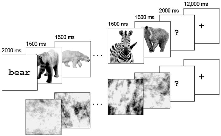
Two trials from the scanning tasks. The first is a catch trial from the mammals task; the target animal is bear, and a zebra intrudes in the sequence. The second is a non-catch trial from the visual baseline task (phase-scrambled images of bears); the pound sign is absent from the images. In the first case, the participant would respond at the question mark; in the second, she would give no response.

The last functional run of the experiment employed phase-scrambled versions of the mammal images used earlier. (Phase scrambling preserves only the amplitudes of the Fourier spectrum of an image; see Fig. 1.) Some of the scrambled images were marked with a small, low-contrast pound (#) sign randomly placed in the image. All stimuli were displayed using E-PrimeTM presentation software (Psychology Software Tools, Pittsburgh, PA).

1.3. Design

Our design relied on a task that exercises concept identification without explicitly requesting judgments of similarity. Specifically, we asked participants to detect “intruders” in a sequence of images of a given mammal category.

In the fMRI phase of the study, participants completed eight functional runs; the first seven are termed the “mammal task,” the last the “visual baseline task.” The trials composing a run were of two kinds: normal trials in which no intruder appeared, and catch trials in which a sole intruder did appear. Normal trials invited no response and figured in our similarity analysis; catch trials served only to ensure attention, and were discarded. Specifically, each run of the mammal task was composed of 9 trials divided between normal and catch; each normal trial presented the name of one mammal followed by its 8 images randomly ordered, with a response interval at the end. Catch trials in the mammal task differed from normal trials only in the replacement of one image by an intruder.

Each run of the mammal task (composed of 9 trials, one per mammal) totaled 264 s including rest. The mammals in a given run were presented in different counterbalanced orders for different participants. Catch trials occupied one, two, or three of the trials in a given run of the mammal task. Trials were arranged so that for each mammal the experiment produced data from six normal trials.

The single run of the visual baseline task included eleven trials. Nine trials contained the scrambled images of a single target mammal. Two trials contained the scrambled images of an intruder mammal; these were catch trials. The pound sign appeared once in each catch trial, never for target mammals. Thus, for each of the nine target mammals, the phase-scrambled images were viewed once. Catch trials were again excluded from analysis.

1.4. Procedure

The experiment began by familiarizing the participant with all stimuli, and practicing the experimental tasks using birds instead of mammals. Participants then proceeded to the scanning and similarity-rating phases, in that order.

1.4.1. Scanning phase

The scanning phase consisted of the seven runs of the mammal task followed by the single run of the visual baseline task. Each trial in the mammal task was composed of three consecutive segments: Name, Sequence, and Response. The Name segment consisted of one of the target animal names, presented for 2 s. The Sequence segment consisted of eight animal images, presented contiguously for 1.5 s each, totaling 12 s. The Response segment displayed a question mark on the screen for 2 s. In a given trial, the participant verified whether each image was an instance of the category presented in the Name segment; for example, if the name was “bear,” the participant verified whether all eight subsequent pictures were bears. If an image failed to match its name (an intruder in a catch trial), the participant pressed a key during the Response segment; for matches (normal trials), participants made no response. Between trials and at the beginning and end of the run, subjects received a 12-s rest period to allow the signal to return to baseline. See the top of Fig. 1 for a summary of one trial.

During the visual baseline task no names were presented. Instead, participants searched the images for a pound (#) sign. If it was detected, they pressed a key during the Response segment, and otherwise did nothing. See the bottom of Fig. 1. Once again, images were presented contiguously for 1.5 s each, totaling 12 s, followed by a 2-s response interval. Note that only catch trials involved a response, and these were not analyzed. Subjects were 100% accurate at detecting catch trials both in the main task and the visual baseline.

In what follows, reference to mammals should be understood as “target mammals”; the intruders are no longer considered.

1.4.2. Similarity-rating phase

After scanning, participants were given a deck of 36 cards. On each card was printed a pair of target mammal names and four images of each of the two mammals (no mirror images). There was one such card for each of the 36 possible pairs of the nine target mammals. Participants were directed to rank the pairs in order of the similarity of the mammals shown; we specified that ranks should not be based on the visual similarity of the images, but rather on the conceptual similarity of the animals represented. Subsequent to ranking, subjects wrote numerical values on the cards to construct an interval scale of perceived similarity. No mention of similarity was made until participants entered the similarity phase of the study.

1.5. Image acquisition

Scanning was performed with a 3-Tesla Siemens Allegra fMRI scanner. Participants’ anatomical data were acquired with an MPRAGE pulse sequence (176 sagittal slices) before functional scanning. Functional images were acquired using a T2-weighted echo-planar pulse sequence with thirty-three 64 × 64-voxel slices, rotated back by 5° on the left–right axis (axial–coronal −5°). Voxel size was 3 mm × 3 mm × 3 mm, with a 1-mm gap between slices. The phase encoding direction was anterior-to-posterior. TR was 2000 ms; time to echo was 30 ms; flip angle was 90°. Field of view was 192 cm × 192 cm.

1.6. Image analysis and regions of interest

Using AFNI (Cox, 1996), functional data were registered to the participant’s anatomical MRI. Transient spikes in the signal were removed (AFNI’s 3dDespike) and data were spatially smoothed using a Gaussian kernel with 6-mm full width at half maximum, and normalized to percent signal change. For each participant, multiple regression was used to generate parameter estimates, called β below, representing each voxel’s activity in each mammal condition and each visual baseline condition. To calculate β, all variables were convolved with a canonical, double gamma hemodynamic response function and entered into a general linear model. Motion estimates were included as regressors of no interest; catch trials were discarded by removing them from the data. In a given voxel, the activation level for mammal m is defined as the β value for m’s mammal condition minus that for m’s visual baseline.

The 12 resulting activation maps for a given mammal (one for each subject) were projected into Talairach space and averaged, leaving us with nine such maps, one for each mammal. Voxels in these Talairach maps measured 1 mm on a side with no separations. Only voxels present in the intersection of all subjects’ intracranial masks were considered. These nine maps show a given voxel’s average activation level for each mammal. (In addition to these averaged maps, the similarity analysis discussed below is also applied to the mammal maps of individual subjects.)

Independently of these activation maps, we used ANOVA to localize voxels containing information about the stimuli. Specifically, we conducted a 2 × 12 ANOVA comparing two sets of regression coefficients, one quantifying a voxel’s response to all intact pictures, and the other its response to all scrambled pictures. The first factor was thus intact versus scrambled images (treated as a fixed effect); the second was subjects (random effect). (The coefficients were obtained via a GLM procedure with two regressors of interest: intact versus scrambled stimulus.) The map was thresholded at F(1,11) = 19.75 (p < 0.001) and clustered based on adjacency of voxel faces. In detail, voxels v₁ and v₂ were considered to be in the same cluster just in case they satisfied the following recursive definition: (a) v₁ and v₂ shared a face or (b) v₁ shared a face with a voxel in a cluster containing v₂. The foregoing procedure ensures that each voxel inhabits at most one cluster in a given map. Clusters smaller than a milliliter were discarded, leaving six clusters to serve as functional regions of interest (fROIs; see Table 2). (The largest cluster excluded was 778 voxels, less than half the size of the smallest one reported; several other yet smaller clusters were also excluded.)

Table 2.

Locations and prediction scores of ANOVA-defined clusters.

Gyrus	BA	SqD	PC	# voxels	x	y	z
Left MOGa	19/37	0.65	0.61	1868	−47	−71	1
Right MOG/FFG/ITGa	19/37/20	0.59	0.40	7914	47	−60	−7
Right insula/IFGb	13	−0.14	0.00	1953	42	15	4
Left precentral gyrusb	6	−0.13	−0.03	1645	−29	−8	51
Left cuneusb	18	0.00	0.00	1590	−25	−77	18
Bilateral visualb	18/30	−0.06	−0.03	21,925	2	−67	4

The clusters shown here were produced from the intact versus scrambled contrast (which quantifies with an F statistic each voxel’s differential activation to all intact versus all scrambled pictures). The x, y, and z coordinates show centroids for each cluster. The map was thresholded to retain only voxels with F-scores yielding p < 0.001. Surviving voxels were assigned cluster identities based on adjacency of voxel faces. Small clusters (<1000 voxels) were discarded. Voxels measure 1 mm per side. Bolded correlations are significant by t-test at p < 0.001. The italicized correlation is significant at p < 0.05.

^aThese voxels responded more strongly to intact than to scrambled images (t(11) > 4.44, p < 0.001).

^bThese voxels responded more strongly to scrambled than to intact images (t(11) <−4.44, p < 0.001).

We attempted to use activation patterns in the six fROIs to predict ratings of similarity, as explained shortly. First observe that our localization technique merely selects voxels that respond differently to intact versus scrambled images. It is thus blind to the identity of the mammals, and cannot bias subsequent analyses in favor of predicting similarity. Indeed, a given voxel could respond identically to all the intact mammals yet still be selected by the localizer (it suffices that this voxel give a different response to scrambled mammals).

1.7. Predicting similarity: general strategy

Each participant’s similarity ratings were linearly normalized to run from 0 (least similar pair) to 1. The 12 resulting scales were then averaged. We attempted to predict these 36 average similarities (one for each pair drawn from the 9 mammals) by correlating them with neural similarity.

Various definitions of neural similarity are discussed below. In all cases, a pattern of activation in a given fROI is identified with a real vector of length equal to the number of its voxels. The ordering of voxels is arbitrary but understood to be the same for all patterns. The proximity between the vectors for two mammals is then quantified and compared to rated similarity.

We begin with techniques that directly compare the activation vectors evoked by the 9 mammals. We then consider a technique based on linear separability of the activations arising from a given pair of mammals.

1.8. Predicting similarity using measures of vector proximity

Our first measure of neural similarity relies on the squared deviation between the respective vectors v(m), v(n) for mammals m and n (each containing l voxels, where l is the size of the given fROI). Specifically, we compute ${\sum }_{i=1}^l{(v_i(m)-v_i(n))}^2$ where v_i(m) is the ith coordinate of v(m), and likewise for v_i(n). Before measuring squared deviation in an fROI, we mean-corrected each pattern by subtracting its mean activation value from each β value in the pattern. This ensures that our neural distance measure is insensitive to mean differences in the fROI. To extract proximity from squared deviation (which measures distance), we normalized all 36 squared deviations (one for each pair of mammals) to the unit interval, then subtracted each normalized score from 1. We denote this proximity measure (based on squared deviation) by “SqD.” The second proximity measure was the Pearson correlation between the vectors v(m), v(n) corresponding to mammals m and n. Pearson correlation employs z-scores instead of raw values, so no additional mean correction is required. This proximity measure is denoted by “PC.”

These measures of neural proximity were applied to the 9 mammal maps obtained from averaging data from the 12 subjects (as described above). They were also applied to the data from each subject individually.

1.9. Predicting similarity using linear separation

An additional measure of neural similarity used the classification error of a support vector machine (SVM) with linear kernel. For this purpose, we relied on the SVM package implemented in R, based on LIBSVM (Chang & Lin, 2001).

To describe this method, we first note that every voxel was sampled 132 times in a given run, yielding 132 zero-centered percent signal change values. Each of these 132 values was divided by the sample standard deviation to obtain z-scores. All z-scores greater than 2 were reset to 2, and likewise for z-scores below −2 (less than 5% of z-scores were so truncated). For a given TR, we call the vector of z-scores across all voxels in the given fROI a time point for m. Thus, a time point is a vector of z-scores, one z-score for each voxel in the given fROI during the given TR. For each subject there are 36 time points per mammal (arising from six non-catch trials with six time points per trial), hence 432 such time points over all 12 subjects.

For each pair of mammals m, n, we submitted all of their 864 time points (432 per mammal) to the linear SVM and observed the number of classification errors committed by the best separating hyperplane. The number of errors serves as our measure of similarity between m and n (i.e., less separable categories were considered more confusable hence more similar).

We add a technical note. Signal change was computed from activity occurring 6 s after the corresponding stimulation. This shift compensates for hemodynamic lag; see, e.g., Polyn et al. (2005). These values were warped to Talairach space and then downsampled back to 3 mm × 3 mm × 4 mm resolution. Warping to standard space was necessary for across-subject consistency in the number and location of voxels submitted to SVM, while downsampling made the problem computationally tractable.

2. Results

2.1. Behavioral data

Descriptive statistics for rated similarity are displayed in Table 1. For each pair of the twelve subjects, we computed the correlation between their similarity judgments (66 correlations in all). The average correlation was 0.54 (SD = 0.22, median = 0.59), indicating significant agreement among participants.

Table 1.

Means and standard deviations of rated similarity among mammals.

		Mean	SD
Cougar	Lion	0.97	0.06
Camel	Horse	0.80	0.21
Elephant	Hippo	0.78	0.21
Giraffe	Horse	0.75	0.21
Bear	Lion	0.73	0.14
Camel	Giraffe	0.71	0.23
Bear	Cougar	0.71	0.12
Camel	Elephant	0.62	0.21
Elephant	Giraffe	0.61	0.31
Hippo	Horse	0.60	0.27
Elephant	Horse	0.60	0.21
Bear	Hippo	0.57	0.26
Bear	Horse	0.54	0.14
Camel	Lion	0.51	0.19
Horse	Lion	0.50	0.23
Giraffe	Lion	0.46	0.25
Bear	Elephant	0.46	0.16
Giraffe	Hippo	0.45	0.26
Camel	Hippo	0.45	0.14
Elephant	Lion	0.45	0.16
Bear	Camel	0.44	0.17
Camel	Cougar	0.43	0.20
Cougar	Horse	0.43	0.17
Dolphin	Hippo	0.42	0.31
Cougar	Giraffe	0.40	0.21
Hippo	Lion	0.40	0.19
Cougar	Elephant	0.38	0.19
Cougar	Hippo	0.33	0.23
Bear	Giraffe	0.29	0.14
Dolphin	Elephant	0.23	0.23
Dolphin	Horse	0.19	0.21
Bear	Dolphin	0.19	0.22
Cougar	Dolphin	0.15	0.18
Camel	Dolphin	0.13	0.18
Dolphin	Giraffe	0.13	0.16
Dolphin	Lion	0.11	0.10

Data are ordered from maximum to minimum average similarity. Similarities were calculated by linearly normalizing each subject’s data to the unit interval and taking the mean; standard deviations across the 12 subjects were generated from these normalized similarities.

Although voxel-wise squared deviation possesses metric properties, it is sometimes disputed that the same is true of rated similarity—or rather, its inverse, distance (Tversky & Gati, 1978, but see Aguilar & Medin, 1999). To check the averaged similarity ratings for metricity, we submitted them to multidimensional scaling (via principal coordinates analysis as implemented in R; see Gower, 1966). Euclidean distance in the two-dimensional solution correlates with rated similarity at −0.95, suggesting that our subjects’ judgments were very close to metric. The solution neatly arrayed the nine mammals along two dimensions that seem to correspond to ferocity and ratio of limb length to height. The latter ranged from limb-challenged dolphins to spindly camels and giraffes.

Some further points about rated similarity are worth making. Twelve additional subjects were asked for the same 36 similarity judgments described above; their answers were individually normalized then averaged (just as for the ratings of the 12 original subjects). The correlation between similarities from the two different groups of subjects is 0.92, suggesting the robustness of similarity judgment. A third group of 15 subjects rated the 36 pairs of mammals along the criteria of “visual (shape) similarity” and “biological (DNA) similarity,” in contrast with the “conceptual similarity” requested of the previous two groups. Normalization and averaging were performed as before. The correlation between conceptual similarity (as rated by our fMRI subjects) and visual similarity (rated by the third group) is 0.94; that between conceptual and biological similarity is 0.92. It is thus difficult to distinguish conceptual/biological from visual similarity in our data. Indeed, the limb length dimension observed in the scaling solution for conceptual similarity has an obvious visual character.¹

2.2. Results using measures of vector proximity: averaged data

We start with the result of averaging the data (both behavioral and neural) across our 12 participants. Analysis at the individual level is reported subsequently. In both cases, the predictive success of SqD and PC was quantified using Pearson correlation with rated similarity.

Our 2 × 12 ANOVA revealed the six fROIs described in Table 2. An fROI in the left middle occipital gyrus (MOG) yielded neural distances that were well correlated with rated similarities under both SqD (r = 0.65, p < 0.001) and PC (r = 0.61, p < 0.001). A roughly homotopic fROI in the right hemisphere (but extending into the fusiform and inferior temporal gyri, called FFG and ITG respectively) predicted well under SqD (r = 0.59, p < 0.001) and somewhat less well under PC (r = 0.40, p < 0.05). These results are also significant by permutation test, in which mammal names are permuted in the behavioral data prior to recomputing the correlation between rated and neural similarity; 1000 trials of this nature produced correlations as high as the four just reported only 0.4%, 1.7%, 0.1%, and 3.5% of the time, respectively. Scatter plots for the four correlations are shown in Fig. 2. We note that the hemodynamic response of both fROIs (left and right MOG) was greater to intact compared to scrambled images (t(11) > 4.44, p < 0.001). When the voxels from the two fROIs were pooled and jointly submitted to SqD and PC, prediction continued to be successful (r = 0.65 and 0.51, with p < 0.001).

Fig. 2.

Scatter plots of prediction results. Two fROIs overlapping the middle occipital gyrus bilaterally predict rated similarity via SqD and PC. Each point in a scatterplot represents neural similarity (the abscissa value) and behavioral similarity (the ordinate value) for a single pair of the 9 mammals. Neural similarities have been normalized to the unit interval.

The ANOVA yielded four additional fROIs in (a) the right anterior insula and inferior frontal gyrus, (b) the left precentral gyrus, (c) the left cuneus, and (d) lingual gyri and retrosplenial cortices bilaterally. None of these fROIs yielded neural distances that predicted similarity ratings under either of our metrics (correlations ranged from r = −0.14 to r = 0.0; see Table 2). Notably, all four of these fROIs responded more strongly to scrambled than to intact images (t(11) < −4.44, p < 0.001), the reverse pattern compared to the two predictive fROIs.

Fig. 3 shows squared deviation for six pairs of mammals in one axial slice of the predictive fROIs. The top row shows the pairs ❬bear, hippo❭ and ❬bear, elephant❭ (both rated as dissimilar), followed by ❬hippo, elephant❭ (rated as similar). We see greater squared deviation in the dissimilar pairs compared to the similar one. The bottom row exhibits the same tendency for dolphin, lion, and cougar. Notice that it is the posterior aspect of the fROIs that discriminates bear from hippo and elephant, whereas the lateral aspect discriminates dolphin from cougar and lion. This suggests that large portions of the fROIs code information about mammals, with the specific region emerging in a given comparison depending on the site of the information most discriminative of the mammals compared. A coronal slice at y = −68 for each of the 9 average activation maps is provided in Fig. 4.

Fig. 3.

Squared deviation of group data in an axial slice of the two predictive clusters (z = 1). Colors are used to code the squared deviation between each voxel’s responses to the two mammals in a given pair. Cold colors signify little or no deviation (small neural distance); hot colors signify the contrary. (Thus, the maps do not directly mark the neural site of any mammal.) The right column reveals little deviation for the behaviorally similar pairs ❬elephant, hippo❭ and ❬cougar, lion❭. The left and middle columns show larger deviations for the dissimilar pairs ❬bear, elephant❭, ❬bear, hippo❭, ❬cougar, dolphin❭ and ❬lion, dolphin❭.

Fig. 4.

Average activation maps for the 9 mammals. This coronal slice (y = −68) portrays the average activations within the slice for each of the 9 mammals in left/right MOG and ITG. These are the two fROIs that responded more vigorously to intact compared to scrambled images of the mammals.

Our prediction results might have been driven by low-level stimulus properties. To test this possibility, we derived inter-image similarities from pixelwise Euclidean distance (Eger, Ashburner, Haynes, Dolan, & Rees, 2008). Specifically, for each mammal m we generated an average image via the following procedure. For each pixel we subtracted its mean intensity across m’s eight scrambled images from its mean intensity across m’s eight intact images. This mirrors the averaging and subtraction used to generate voxel activations, and produces one average image per mammal. We then calculated the Euclidean distance between average images for every pair of mammals. Next, these distances were converted to similarities by linear normalization to the unit interval followed by subtraction from unity (just as SqD was converted to similarity). Substituting image-derived similarity for rated similarity, we reran the SqD and PC analyses. None of our six fROIs showed significant correlation with image-derived similarity under either SqD or PC (maximum r = 0.29; p > 0.05).

2.3. Results using measures of vector proximity: individual data

To define fROIs at the individual level, we performed a general linear test on each participant, contrasting all intact with all scrambled images. In each case, voxels discriminating intact from scrambled images at p < 10⁻⁵ were clustered. Clusters most closely corresponding to the two predictive fROIs found at the group level (namely, left/right MOG) were used to predict a given participant’s rated similarity. (Unsmoothed data were used to derive activation levels in individual participants; smoothing yields qualitatively similar results but not as trenchant.)

Of the 12 participants, 11 yielded an fROI corresponding to right MOG and 10 yielded one corresponding to left MOG. The SqD metric showed no strong association between individual MOG activity and individual similarity. PC produced a 0.32 median correlation (range = −0.35 to 0.53) in left MOG, with nine of 10 correlations positive and five significant (p < 0.05, 34 d.f.). A sign test of the hypothesis of zero median yields p < 0.02. PC gave a median correlation of 0.18 in right MOG (range = −0.24 to 0.48) with 10 of the 11 correlations positive (p < 0.01 by sign test). Only one is significant. Fig. 5 displays the locations of the individual fROIs that yielded the median and highest correlations with rated similarity; scatter plots are also shown.

Fig. 5.

Locations and scatterplots for median and best results from individual analyses. (a) The individual subjects yielded a median correlation with judged similarity of 0.32 near left MOG. Shown are the voxels that produced this result and the similarity predictions induced by those voxels in the two median subjects (z = −13 in both cases, with centroids (−40, −70, −8) and (−46, −65, −4) respectively). (b) The best individual correlation with judged similarity from an area near right MOG was 0.48; the best correlation near left MOG was 0.53. (These results originated from different subjects.) For right MOG, z = −4; for left, z = −10. Centroids were (50, −65, −5) and (−48, −69, 4) respectively.

We see that our group findings are partially recapitulated at the individual level. There is a positive relationship between neural similarity (defined by PC) and behavioral similarity. Still, averaging both the neural and behavioral data produces higher correlations than seen for individual subjects.

2.4. Results based on linear separation

Recall that for mammals m, n, similarity was here measured by the classification error of the best separating hyperplane for the two sets of 432 time points corresponding to m and n. As fROIs we considered only left/right MOG (since they alone responded more strongly to intact compared to scrambled images). For right MOG (two-hundred and forty-one 3-mm voxels), we observed a correlation of 0.417 between rated similarity and classification error (p < 0.02). A scatter plot is given in Fig. 6. If we omit the truncation of z-scores beyond ±2 (see above), the correlation falls to r = 0.375 (p < 0.03). The correlation for left MOG (fifty-six 3-mm voxels) is not significant (r = 0.061).

Fig. 6.

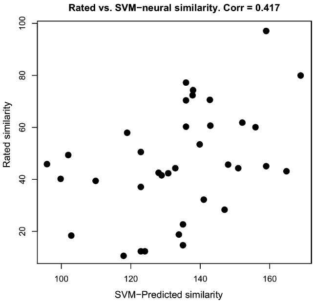
Scatterplot for linear separation analysis. Each point represents one pair of mammals. The abscissa shows average rated similarity of a given pair whereas the ordinate shows the number of misclassifications (out of 864 time points) committed by the best separating hyperplane for that pair. The correlation of 0.417 is significant at p < 0.02.

To illustrate, when attempting to separate lion from cougar (animals rated as highly similar), 18.4% of the time points were misclassified by the linear SVM. Classification was more successful for the less similar pairs cougar versus giraffe (11.6% misclassified) and lion versus giraffe (11.1%). In general, linear separation of one mammal representation from another was largely successful. Given a pair m, n of mammals, let the classification accuracy denote the percentage of time points for m or n that were correctly classified by the linear SVM. Across the 36 pairs, classification accuracy ranged from 80.44% to 88.89% with mean 84.49% (SD = 2.09%).

The linear separability of different mammals was too accurate to allow application of our SVM technique to individual subjects (36 time points per mammal). This is because classification is virtually perfect for all subjects with respect to all pairs of mammals, thus eliminating variation among mammal pairs on this measure of neural similarity.

3. Discussion

We have proposed simple measures of the similarity of neural representations of categories. Two of these measures compare the response of each voxel in a given fROI to images of different mammals; one relies on squared deviation for this purpose, the other uses correlation. When applied to regions with greater signal change to intact versus scrambled images of mammals (left/right MOG), both methods correlate significantly with rated similarity. (The ratings were collected after scanning.) Results were better if based on averaged data from our 12 subjects, compared to treating each data set separately. We attribute this to noise cancelation at the group level, allowing common tendencies to emerge more clearly (albeit obscuring important idiosyncratic aspects of object representation).

A third measure of neural similarity relies on the collection of time points generated by each subject viewing a given mammal during a given run. For each pair m, n of mammals, we applied a support vector machine with linear kernel to obtain the hyperplane that best separates the time points of m and n. The number of misclassified points served as a measure of neural similarity (“confusability”). When applied to right MOG, this measure correlates reliably with rated similarity. (Right MOG is the largest cluster that responds more vigorously to intact versus scrambled images.) Note that this third measure does not average neural data between subjects.

Our results complement a recent study by Eger et al. (2008), who found that support vector machines discriminate between category exemplars (e.g., various types of chairs) in regions closely overlapping those reported above (namely, the lateral aspect of the occipital cortex). Although Eger et al. (2008) do not consider similarity judgments, the convergence of the two studies on the same region strengthens the case in favor of shared neural substrata for distinct concepts.

We have aimed for simplicity in constructing our three techniques for predicting rated similarity. Many alternatives were nonetheless examined (for example, cosine as a measure of vector similarity) but none performed better than SqD and PC. Likewise, we tried more sophisticated kernels for the SVM (notably, polynomial and radial basis) but only the linear kernel offered significant correlations with rated similarity. This suggests a relatively simple organization of mammal representations in right MOG.

We defined fROIs on the basis of their voxels’ differential response to intact versus scrambled images. We did not attempt to base fROIs on voxels’ response to categories that contrast with mammal, such as fruit or vehicle. Such contrasts might yield fROIs predictive of similarity. But they may also fail to identify voxels that are responsive to common features of the contrasting categories and thus miss voxels that participate in intra-category similarity (see Gerlach, 2007).

The two predictive fROIs (and the only clusters that showed greater hemodynamic response to intact versus scrambled pictures) largely overlap a functionally defined region known as the lateral occipital complex (LOC). Several studies reveal the LOC to be more sensitive to images with clear shape interpretations than to scrambled images presenting no clear shape (Grill-Spector, Kourtzi, & Kanwisher, 2001; Larsson & Heeger, 2006; Xu & Chun, 2006). Similarity based on shape may thus underlie the predictive success of our two fROIs if rated (“conceptual”) similarity is likewise dominated by the shape of mammals. Given the high correlations reported above among ratings of conceptual, visual, and biological similarity, the present data do not pinpoint the kind of representation encoded in the LOC.

In considering this issue, it is well to distinguish the similarity of mammal pictures from subjects’ judgments of the visual similarity of the mammals themselves. The latter is evoked, but not driven, by the stimuli, which were two-dimensional images representing a variety of poses, camera angles, and exemplars. (Compare, for example, the brown bear and the polar bear shown in Fig. 1, and recall that pixelwise and neural similarity were uncorrelated.) Our findings thus suggest that conceptual knowledge (visual or otherwise) helps determine the representation of categories in the LOC.

This idea is consistent with the findings of Stanley and Rubin (2005), who showed that anterior LOC distinguishes familiar objects from abstract shapes, and with those of Haushofer, Livingstone, and Kanwisher (2008), who report that activity in a nearby region reflects perceptual more than physical similarity of abstract shapes. Our results extend these observations by demonstrating that LOC activity reflects the fine-grained similarity structure within at least one familiar concept (mammals).

We have shown that measures of neural proximity can be used to recover rated similarity even when those measures are applied to brain activity evoked by nothing more than category verification. Our findings may therefore help to clarify the role of similarity judgment in cognition. Hume (1777) conjectured that induction proceeds from similarity: “From causes, which are similar, we expect similar effects.” Thus, the similar natures of wolves and foxes lead us to expect that they share many biological properties. Hume’s dictum seems more relevant to similarities within natural kinds like mammals, rather than to disparate collections that include fish and planes, or cats and bottles (as examined in Edelman et al., 1998; O’Toole et al., 2005); for, the causal mechanisms responsible for properties in one mammal might well be present in another whereas this is less likely for heterogeneous categories. The present study may thus be more relevant than its predecessors to fundamental questions about induction. Indeed, recent theorists including Goodman (1972) and Murphy and Medin (1985) suggest that Hume had it backwards inasmuch as rated similarity is built on covert estimates of inductive inference—greater similarity accrues to items X, Y that elicit inferences of the form “X has property P therefore Y probably does too.” But note that our fMRI task involved neither similarity nor probability. Subjects merely classified images, with no mention of similarity until scanning was complete; inductive inference was therefore unlikely to have occurred. Yet two areas in the ventral visual stream predicted similarity ratings using plausible metrics of neural resemblance. Our findings thus highlight the possibility that intuitions about similarity are likewise generated without mediation by inductive judgment, based rather on the overlap of mental representations.

References

- Aguilar CM, Medin DL. Asymmetries of comparison. Psychonomic Bulletin & Review. 1999;6:328–337. doi: 10.3758/bf03212338. [DOI] [PubMed] [Google Scholar]
- Averbeck BB, Latham PE, Pouget A. Neural correlations, population coding and computation. Nature Reviews Neuroscience. 2006;7:358–366. doi: 10.1038/nrn1888. [DOI] [PubMed] [Google Scholar]
- Caramazza A, Mahon BZ. The organization of conceptual knowledge: The evidence from category-specific semantic deficits. Trends in Cognitive Sciences. 2003;7(8):354–360. doi: 10.1016/s1364-6613(03)00159-1. [DOI] [PubMed] [Google Scholar]
- Chang C-C, Lin C-J. LIBSVM: a library for support vector machines. 2001 Software available at http://www.csie.ntu.edu.tw/~cjlin/libsvm.
- Cox DD, Savoy RL. Functional magnetic resonance imaging (fMRI) “brain reading”: Detecting and classifying distributed patterns of fMRI activity in human visual cortex. NeuroImage. 2003;19:261–270. doi: 10.1016/s1053-8119(03)00049-1. [DOI] [PubMed] [Google Scholar]
- Cox RW. AFNI: Software for analysis and visualization of functional magnetic resonance neuroimages. Computers and Biomedical Research. 1996;29:162–173. doi: 10.1006/cbmr.1996.0014. [DOI] [PubMed] [Google Scholar]
- Cross K, Smith EE, Grossman M. Knowledge of natural kinds in semantic dementia and Alzheimer’s disease. Brain and Language. 2008;105:32–40. doi: 10.1016/j.bandl.2008.01.001. [DOI] [PMC free article] [PubMed] [Google Scholar]
- Edelman S, Grill-Spector K, Kushnir T, Malach R. Toward direct visualization of the internal shape representation by fMRI. Psychobiology. 1998;26:309–321. [Google Scholar]
- Eger E, Ashburner J, Haynes J-D, Dolan RJ, Rees G. fMRI activity patterns in human LOC carry information about object exemplars within category. Journal of Cognitive Neuroscience. 2008;20:356–370. doi: 10.1162/jocn.2008.20019. [DOI] [PMC free article] [PubMed] [Google Scholar]
- Feeney A, Heit E. Inductive reasoning: experimental, developmental, and computational approaches. Cambridge University Press; 2007. [Google Scholar]
- Franco L, Rolls ET, Aggelopoulos NC, Jerez JM. Neuronal selectivity, population sparseness, and ergodicity in the inferior temporal visual cortex. Biological Cybernetics. 2007;96(6):547–560. doi: 10.1007/s00422-007-0149-1. [DOI] [PubMed] [Google Scholar]
- Gerlach C. A review of functional imaging studies on category specificity. Journal of Cognitive Neuroscience. 2007;19(2):296–314. doi: 10.1162/jocn.2007.19.2.296. [DOI] [PubMed] [Google Scholar]
- Goodman N. Problems and projects. New York, NY: Bobbs-Merrill; 1972. Seven strictures on similarity. [Google Scholar]
- Gower JC. Some distance properties of latent root and vector methods used in multivariate analysis. Biometrika. 1966;53:325–328. [Google Scholar]
- Grill-Spector K, Kourtzi Z, Kanwisher N. The lateral occipital complex and its role in object recognition. Vision Research. 2001;41:1409–1422. doi: 10.1016/s0042-6989(01)00073-6. [DOI] [PubMed] [Google Scholar]
- Haushofer J, Livingstone MS, Kanwisher N. Multivariate patterns in object-selective cortex dissociate perceptual and physical shape similarity. PLoS Biology. 2008;6(7):1459–1467. doi: 10.1371/journal.pbio.0060187. [DOI] [PMC free article] [PubMed] [Google Scholar]
- Haxby JV, Gobbini MI, Furey ML, Ishai A, Schouten JL, Pietrini P. Distributed and overlapping representations of faces and objects in ventral temporal cortex. Science. 2001;293:2405–2407. doi: 10.1126/science.1063736. [DOI] [PubMed] [Google Scholar]
- Haynes J-D, Rees G. Predicting the orientation of invisible stimuli from activity in human primary visual cortex. Nature Neuroscience. 2005;8:686–691. doi: 10.1038/nn1445. [DOI] [PubMed] [Google Scholar]
- Haynes J-D, Sakai K, Rees G, Gilbert S, Frith C, Passingham RF. Reading hidden intentions in the human brain. Current Biology. 2007;17:323–328. doi: 10.1016/j.cub.2006.11.072. [DOI] [PubMed] [Google Scholar]
- Hume D. An enquiry concerning human understanding. Oxford, UK: Oxford University Press; 1777. [Google Scholar]
- Kamitani Y, Tong F. Decoding the visual and subjective contents of the human brain. Nature Neuroscience. 2005;8:679–685. doi: 10.1038/nn1444. [DOI] [PMC free article] [PubMed] [Google Scholar]
- Larsson J, Heeger DJ. Two retinotopic visual areas in human lateral occipital cortex. Journal of Neuroscience. 2006;26(51):13128–13142. doi: 10.1523/JNEUROSCI.1657-06.2006. [DOI] [PMC free article] [PubMed] [Google Scholar]
- Martin A. The representation of object concepts in the brain. Annual Review of Psychology. 2007;58:25–45. doi: 10.1146/annurev.psych.57.102904.190143. [DOI] [PubMed] [Google Scholar]
- Martin A, Wiggs CL, Ungerleider LG, Haxby JV. Neural correlates of category specific behavior. Nature. 1996;379:649–652. doi: 10.1038/379649a0. [DOI] [PubMed] [Google Scholar]
- Murphy GL. The big book of concepts. Cambridge, MA: MIT Press; 2004. [Google Scholar]
- Murphy GL, Medin DL. The role of theories in conceptual coherence. Psychological Review. 1985;92:289–316. [PubMed] [Google Scholar]
- Op de Beeck HP, Torfs K, Wagemans J. Perceived shape similarity among unfamiliar objects and the organization of the human object vision pathway. Journal of Neuroscience. 2008;28(40):10111–10123. doi: 10.1523/JNEUROSCI.2511-08.2008. [DOI] [PMC free article] [PubMed] [Google Scholar]
- O’Toole AJ, Jiang F, Abdi H, Haxby JV. Partially distributed representations of objects and faces in ventral temporal cortex. Journal of Cognitive Neuroscience. 2005;17:580–590. doi: 10.1162/0898929053467550. [DOI] [PubMed] [Google Scholar]
- Polyn SM, Natu VS, Cohen JD, Norman KA. Tracking memory search and retrieval in an fMRI study of free recall. Science. 2005:310. doi: 10.1126/science.1117645. [DOI] [PubMed] [Google Scholar]
- Rogers TT, McClelland JL. Semantic cognition: a parallel distributed processing approach. 1. Cambridge, MA: The MIT Press; 2004. [DOI] [PubMed] [Google Scholar]
- Sloman SA. Feature based induction. Cognitive Psychology. 1993;25:231–280. [Google Scholar]
- Snowden JS, Goulding PJ, Neary D. Semantic dementia: a form of circumscribed cerebral atrophy. Behavioral Neurology. 1989;2:167–182. [Google Scholar]
- Stanley DA, Rubin N. Functionally distinct sub-regions in the lateral occipital complex revealed by fMRI responses to abstract 2-dimensional shapes and familiar objects. Journal of Vision. 2005;5:911a. [Google Scholar]
- Tenenbaum JB, Kemp C, Shafto P. Theory-based Bayesian models of inductive reasoning. In: Feeney A, Heit E, editors. Inductive reasoning: experimental, developmental, and computational approaches. Cambridge, UK: Cambridge University Press; 2007. pp. 167–2004. [Google Scholar]
- Tversky A, Gati I. Studies of similarity. In: Rosch E, Lloyd BB, editors. Cognition and categorization. Hillsdale, NJ: Lawrence Erlbaum; 1978. [Google Scholar]
- Tyler LK, Bright P, Dick E, Tavares P, Pilgrim L, Fletcher P, et al. Do semantic categories activate distinct cortical regions? Evidence for a distributed neural semantic system. Cognitive Neuropsychology. 2003;20:541–559. doi: 10.1080/02643290244000211. [DOI] [PubMed] [Google Scholar]
- Warrington EK. The selective impairment of semantic memory. Quarterly Journal of Experimental Psychology. 1975;27(4):635–657. doi: 10.1080/14640747508400525. [DOI] [PubMed] [Google Scholar]
- Warrington EK, McCarthy R. Categories of knowledge: Further fractionation and an attempted integration. Brain. 1987;110:1273–1296. doi: 10.1093/brain/110.5.1273. [DOI] [PubMed] [Google Scholar]
- Warrington EK, Shallice T. Category specific semantic impairments. Brain. 1984;107:829–854. doi: 10.1093/brain/107.3.829. [DOI] [PubMed] [Google Scholar]
- Xu Y, Chun MM. Dissociable neural mechanisms supporting visual short-term memory for objects. Nature. 2006;440:91–95. doi: 10.1038/nature04262. [DOI] [PubMed] [Google Scholar]