Marker selection for genetic case-control association studies

Abstract

Association studies can focus on candidate gene(s), a particular genomic region, or adopt a genome wide association approach, each of which has implications for marker selection. The strategy for marker selection will affect the statistical power of the study to detect a disease association and is a crucial element of study design. The abundant single nucleotide polymorphisms (SNPs) are the markers of choice in genetic case-control association studies. The genotypes of neighbouring SNPs are often highly correlated (‘in linkage disequilibrium’ – LD) within a population which is utilised for selecting specific ‘tagSNPs’ to serve as proxies for other nearby SNPs in high LD. General guidelines for SNP selection in candidate genes/regions and genome-wide studies are provided in this protocol, along with illustrative examples. Publicly available web-based resources are utilised to browse and retrieve data and software such as Haploview and Goldsurfer2, are applied to investigate LD and to select tagSNPs.

Introduction

The human genome consists of over 3 billion base pairs and was sequenced as part of the Human Genome Project that started in 1990. The ‘final’ version of the sequence was published in 2003, and estimated at the time to be 92% complete¹. It showed that the human genome consists of ~ 22,000 genes (see Box 1 for a glossary of terms), and that human individuals are identical for ~99.5% of their sequence, with the small remaining part variable to differing extents. Since this variation could have an important role in explaining differences in genetic susceptibility to disease, comparing variation between diseased (cases) and healthy (control) individuals from the same population may elucidate which genetic pathways are involved in disease onset and progression ².

Box 1. glossary.

Allele

a variant of a polymorphism at a locus

Enhancer

a regulatory region of the DNA to which proteins can bind in order to increase the expression of a gene

Exon

a section of a gene that is represented in the mature form of the mRNA transcript

Gene

a functional unit of DNA that contains the necessary information for the cell machinery to create a RNA template that is either functional by itself or can be translated to a protein

Genotype

the combination of two alleles across both chromosomes at a particular locus in an individual

Haplotype

a consecutive sequence of alleles at different loci on a single chromosome in an individual

HapMap

An international project to develop a haplotype map of the human genome. The publicly available data consist of ~3.2 million common SNPs genotyped in four different sample sets of 60-90 individuals with African, Asian and European ancestry. Frequently used as reference data for designing and following up genetic case control studies.

Intragenic region

a section of the genome that lies between genes

Intron

a non-coding section of a gene that is removed from the mature mRNA sequence by a process called splicing

Linkage Disequilibrium (LD)

The population correlation between two (usually nearby) allelic variants on the same chromosome; they are in LD if they are inherited together more often than expected by chance.

Regulatory region

a section of DNA sequence that directly or indirectly affects the expression of a gene

Promoter

a regulatory element often located immediately upstream of the gene whose expression it regulates

Single Nucleotide Polymorphism (SNP)

a genetic variant that consists of a single DNA base pair change, resulting in two possible allelic identities at that position

tagSNP

a SNP in a region of the genome featuring high LD, which is a proxy for others in close proximity and which can be used to genotype individuals at a reduced cost whilst maintaining power

Untranslated Region (UTR)

A section of the mRNA transcript that is not translated to aminoacid sequence. Two examples of such regions are the 5'UTR and the 3'UTR, which are located before and after the coding parts of the transcript, respectively.

Genetic variation at a specific locus is termed a polymorphism if it occurs with a frequency > 1% in the population, and a mutation if it occurs less frequently ³. The most common class of polymorphisms involve a single base-pair change, also termed single nucleotide polymorphisms (SNPs), which comprise ~90% of all human variation. Other types of polymorphism include larger blocks of sequence variation (mini/micro-satellites) or more complex alterations of the sequence such as inversions and deletions, or copy-number variations (CNVs) ⁴. The different variations that a polymorphism can have at a particular locus are termed alleles. For SNPs, the single base pair changes occur predominantly within the two classes of nucleotides, between purines (A ↔ G) or pyrimidines (C ↔ T), which means that most SNPs will only have 2 alleles in a population. The specific combination of these alleles in an individual counting across the two relevant chromosomes is referred to as a genotype. In contrast, the combination of consecutive alleles on a single chromosome is termed a haplotype.

The potential of using these abundant SNPs in association studies motivated a large-scale international cataloguing effort, the SNP Consortium ⁵. The database used for submission, dbSNP, currently holds >10 million SNPs. Conducting association studies by genotyping samples for all known polymorphisms is not financially feasible nor necessary: various studies showed that alleles of SNPs located close together on a chromosome are not inherited independently within a population, but are correlated, such that many individuals share the same haplotype (haplotype blocks) ⁶. This correlation between genetic variants within a population is termed ‘linkage disequilibrium’ (LD), and it is this feature that is utilised in marker selection.

The international HapMap project was initiated to characterise LD across the human genome. In phase I of the study ~1 million common SNPs were genotyped in four different sample sets of 90 Yoruba in Ibadan from Nigeria (YRI), 45 Japanese in Tokyo Japan (JPT), 45 Han Chinese in Beijing China (CHB) and 60 CEPH (Utah Residents with Northern and Western European Ancestry)(CEU) ⁷. The study confirmed that alleles of neighbouring SNPs are often highly correlated within a population of unrelated individuals, and that specific ‘tagSNPs’ ⁸ can be selected to serve as proxies for other SNPs in high LD, thus substantially reducing the number of SNPs that need to be genotyped in order to recover most of the information about common variation. The HapMap project provided a map of the LD structure across the genome, together with general statistics for markers such as location and allele frequencies, which allow investigators to select tagSNPs that best capture the common genetic variation in a particular region, or across the genome. HapMap Phase II increased the number of SNPs genotyped in the four populations to ~ 3.2 million ⁹; phase III extends the information to an additional seven populations but at a limited number of SNPs (http://www.hapmap.org). Due to the relatively small number of individuals genotyped in the HapMap project - 60 unrelated individuals genotyped in each population sample - only relatively common polymorphisms (with frequency > 0.02) can be captured. However, detecting the influence of rare variation underlying common disease through population-based case-control studies - even with 1000s of cases and controls is difficult, unless effect sizes are very large ².

When utilising the HapMap data as a reference for the selection of SNPs for a genetic association study it is important to be aware that the genotypes and associated statistics are based on the characterized sample populations and may not be directly transferable to the individuals in a given study. Thus, investigators should view summary statistics for the HapMap population which they believe is most similar in terms of ancestry to the study population. Also, certain SNPs will either not have been genotyped in HapMap or may be monomorphic in the HapMap population of 60 individuals. Better characterisation of such SNPs may be based on a more complete resource such as dbSNP, although this database has the limitation that SNPs may not have been validated and that no genotype data is publicly available. For studying specific candidate regions other publicly available SNP databases such as SeattleSNPs (http://pga.mbt.washington.edu/) and GeneSNPs (http://www.genome.utah.edu/genesnps/) sometimes offer better coverage since they contain genotype information from resequencing of genes or candidate regions. An international collaborative effort launched in 2008, The 1000 Genomes Project aims to resequence 1000 individuals using third generation high-throughput resequencing technologies (http://www.1000genomes.org). The outcome of this project will greatly facilitate the follow up of genetic studies and will be a main resource for the development of new analytical and experimental methods.

The types of genetic association studies conducted are commonly divided into candidate gene/region and genome-wide association studies. Both of these approaches involve genotyping SNPs in large collections of cases and controls (the focus of this protocol) or in large collections of individuals characterised by continuous quantitative traits. Although the general principles by which markers are selected in candidate gene vs genome-wide studies are the same, i.e. based on optimal genomic coverage, the investigator-driven methodology that is implemented in a candidate gene/region approach means that in practice they are very different. A candidate gene study is based on a prior hypothesis suggesting a potential role of the gene(s) in a particular phenotype or disease. The support for the selection of a candidate gene or region is typically based on its biological function or on its location in a region implicated in a previous linkage or association study. In a candidate gene study, the aim is to obtain the highest possible coverage of genetic variation within specified genomic boundaries, taking account of any known functional genomic characteristics. In contrast, genome-wide association studies utilise pre-designed genotyping panels containing selected sets of SNPs distributed throughout the whole genome. Genome-wide association studies are useful for hypothesis-generating purposes but rarely provide the same coverage for a candidate region as a well-designed candidate gene study.

Candidate gene/region marker selection

The advantage of performing a study focused on one or few candidate genes or regions is cost efficiency. A relatively small number of markers will need to be genotyped to capture most of the common variation in the candidate region. However, de-novo candidate gene studies, in which candidates are selected entirely on the basis of their supposed biological significance, without any previous statistical evidence that the region they are located in is implicated, have had very low success rates even when well-designed ¹⁰. Candidate gene/region studies should therefore follow genomic linkage or association studies that have already implicated the region. Linkage studies are designed to indicate evidence of relatively rare variants with big effects, whereas association studies are powered to pick up common variants with modest effects. Following up linkage signals with population-based association study might not be the optimal strategy and this needs to be taken into account when selecting both the individuals and the markers to genotype in the follow up study. Alternatively, candidate genes can be selected from biological pathways which harbour other previously associated risk loci. Various types of other data can also be useful to provide further insight on functionality, for example whether a gene is expressed in tissues relevant to the biological mechanism of the disease.

A genetic polymorphism may act by affecting the regulation of expression of the candidate gene or by leading to a changed composition and function of the protein that it encodes. The selection of SNPs in or around the candidate gene region should take account of in-depth characterization of the functional elements identified therein and how their localization in relation to the gene might affect its function. Nevertheless, it is important to note that functional elements both within and outside boundaries of a gene may well be unknown at the time of study, and our knowledge of functionality is expanding continuously. Regulatory regions such as promoters and enhancers are essential for controlling the extent to which the gene is transcribed. Polymorphisms in coding exons and regulatory regions are less frequent than variations in a part of a sequence with no clear functional role such as intergenic regions and introns. This is explained by the fact that altering the function of the fine-tuned biological system will likely have a detrimental effect on the functioning and survival of the individual, the result of which is a smaller likelihood that the variation is passed on and established in the population (although a mutation can also have a positive effect on survival and therefore increase in frequency).

Through customized genotyping, the coverage can be specifically increased for the candidate genes/regions. In addition, the investigator has the opportunity to customise SNP selection, ensuring the inclusion of known functional or rare variants that might have been removed from other commercial panels. Therefore, the first step in SNP selection for a candidate gene or region is to find out relevant genomic information: identify all known SNPs, identify those known to be located in functional regions, and characterise the LD structure, using publicly available online databases such as Ensembl (http://www.ensembl.org), UCSC Genome Browser (http://genome.ucsc.edu) ¹¹, and HapMap (http://www.hapmap.org).

Depending on the size of the candidate region, and the cost implications, the investigator can choose to include all potentially functional SNPs (localised in predicted regulatory regions, splice sites, intergenic sequence, introns or coding exons) in marker selection, supplemented by a selection of tagSNPs, or rely on the use of tagSNPs alone to cover the gene/region. Selecting markers on the basis of functional annotation alone is not recommended, since the causative polymorphism may not have been identified yet, or may be in a region that has to date been deemed ‘non-functional’ ¹². Of course, if a specific study is aimed at replicating and/or fine mapping a candidate region suggested by the results of a previous study, it is imperative that the SNP associated in the original study is included in the design.

A final step in selecting SNPs is, if possible, to check whether there is any evidence that genotyping is at risk of failing. For instance, it is normally considered difficult to genotype or sequence in genomic regions of low complexity, containing numerous repetitive elements. Since the genotyping could fail for some markers in these regions, it is useful to incorporate additional SNPs in order to capture local variation. This is particularly important in a replication study, where the ability to replicate hinges on the genotyping accuracy of the SNP in question. In this situation, it is advisable to include the next most highly associated SNP in high LD (r²>0.7) and/or a SNP in complete LD with the initial hit using data from the original study or HapMap information if samples are of similar ancestry.

When genotyping SNPs in a candidate gene, the number of SNPs to be genotyped is unlikely to exceed the hundreds. Such quantities are usually easily genotyped using low throughput, PCR-based methods ¹³. However, when genotyping a candidate region, the number of SNPs is likely be in the thousands. With increasingly large numbers of SNPs, it will be more cost efficient to conduct genotyping using high throughput array-based products, similar to those used in Genomewide association (GWA) studies. Such custom-made arrays are normally designed as multiplexes with a fixed number of markers that can be genotyped per chip (for example, Illumina's custom arrays are currently designed in panels of up to 1536 SNPs or >7800 SNPs and Affymetrix at present offers solutions for customized genotyping in configurations of 3K, 5K, 10K and 20K markers). The manufacturers of these panels also publish scores indicating the likelihood of genotype failure of individual SNPs on the relevant panel, thus helping the investigator choose a set of SNPs that will suffer minimal failure.

Genome-wide association panels

With recent advances in the efficiency of array-based high-throughput SNP genotyping technology ¹⁴, hundreds of thousands of SNPs are now routinely genotyped on sample sizes necessary to detect the modest genetic effects we expect for complex diseases ². GWA studies have been undertaken to study a wide variety of diseases and phenotypes, often involving big consortia to obtain the necessary sample sizes. The success of recently published GWAs has shown that this approach can be powerful in helping to identify disease related loci ¹⁵. One of the largest published examples highlighting the success of GWA studies was conducted by the Wellcome Trust Case Control Consortium (WTCCC) where 17,000 individuals were genotyped with the GeneChip 500K Mapping Array Set (Affymetrix chip) panel to study seven different diseases ¹⁶. Subsequent studies showed that most of the significant associations in the WTCCC, as well as those found in other GWA studies, could be replicated and are thus very likely to be real. A summary of recent GWA publications attempting to assay at least 100,000 SNPs is available online and lists the results from hundreds of publications with thousands of SNPs significantly associated to a wide variety of diseases and phenotypes (http://www.genome.gov/gwastudies/).

The main difference between currently available GWA panels involves the number of SNPs for which probes are included and the resulting genomic coverage obtained by this selection. Some of the latest panels also contain probes for analysing copy number variations (CNVs), although there are also methods for identifying these in-silico from genotyping intensities. Current commercially available genotyping panels typically range in capacity from 300K up to 1M SNPs but there are also focused panels that only capture a few hundred SNPs. The design of the panels mainly falls into three categories, containing SNPs 1) more or less randomly selected, 2) chosen because they are tagSNPs and 3) chosen as part of a focused selection based on previously implicated functional importance or for lying within or nearby genes that could have a role for different diseases such as cancer. TagSNP panels have been shown to provide better coverage of common variation ¹⁷. An important note is that the calculated coverage by the selection of tagSNPs is currently based on coverage of all common SNPs genotyped in HapMap, not of the remaining unknown genetic variation. Therefore, coverage achieved is likely to be overestimated, and may not necessarily be sufficient for fine mapping and studying specific regions of interest. Data from the ENCODE project, aimed at identifying all genetic variation in 10 selected genomic regions for 48 HapMap individuals, however, showed that HapMap phase II data generally provide a high coverage of all common genetic variation ¹⁸. The 1000 Genomes Project, aimed at uncovering genomic variation in 1000 individuals around the world through resequencing (http://www.1000genomes.org), should enable a more accurate evaluation of coverage.

Between the currently available genotyping panels, aiming for very high coverage at the expense of sample size will result in a decrease rather than an increase of power ¹⁹. Choosing a panel with fewer markers will reduce genomic coverage, but the funds saved by choosing the cheaper panel can instead be spent on genotyping more individuals. This will increase the statistical power to a greater extent than adding more markers would do. In addition, recently published methods enable imputation (prediction) of ungenotyped SNPs based on those that are genotyped, utilising LD structures calculated from HapMap ²⁰. This offers a potentially attractive approach for increasing coverage whilst spending more funds on increasing sample size ¹⁹. However, imputation is not necessarily a successful solution to increase coverage in all situations. Accurate prediction of an ungenotyped marker depends on the availability of an already genotyped marker to act as a proxy. If a SNP does not have any markers in high LD with it, it cannot accurately be predicted. This means in practice that well-covered regions can easily be filled in but poorly covered regions cannot be improved to any major extent. Given that imputation methods utilise the haplotype structure of reference datasets for the inference of genotypes, The 1000 Genomes Project will also contribute highly to our understanding of genotype imputation methods and their accuracy for imputation of polymorphisms of different frequencies.

Another strategy to save funds, which can be spent instead on choosing a greater-coverage genotyping panel or preferably genotyping more cases, is to use publicly available genotyping data for common controls from another study such as the WTCCC project (provided that they have been sampled from the same underlying population as cases and that population structure is investigated and adjusted for at the analysis stage ²). Publicly available controls, however, are likely to have been genotyped on different panels, and if so, imputation would need to be performed to allow combined analyses.

In the current protocol we present two scenarios for SNP selection, involving a candidate-gene and a GWA study, following the example of type 2 diabetes ². Marker selection for the candidate gene approach will centre around the investigation of the influence of PPARG on type 2 diabetes in a population of European ancestry. Since PPARG (rs1801282) was previously implicated in this disease ²¹ we ensure that the associated variant is included in the final marker selection. Although the example shown relates to a candidate gene, the same methods are applicable when selecting markers for a larger candidate region.

Commercially available products mainly differ in the coverage to price ratio, which rapidly changes with the development and release of new panels. In the GWA procedure section of this protocol (see Box 2) we will go through how to calculate the coverage of available genotyping panels for the markers genotyped in the HapMap project. The script that will be used for calculating the coverage implements the algorithm published by Barrett and Cardon ¹⁷. A new release of the HapMap project with a more complete selection of SNPs genotyped for a larger number of individuals is likely to be released in the near future as well as new commercially available genotyping panels. The coverage calculations can easily be repeated for additional panels by running the script provided, using updated reference data and new SNP lists. Guidelines on how to quality-check and analyse generated GWA and candidate gene data will be presented in subsequent Nature Protocols.

BOX 2. Genome wide association study.

Calculating genotyping coverage

• 1| To download a script for calculating coverage (estimate-coverage.pl) and necessary auxillary files go to http://www.well.ox.ac.uk/~carl/gwa/cost-efficiency/. Scroll down to the ‘coverage of genome-wide SNP platforms’ section and download files by clicking on the first four links. If downloading does not start automatically right-click on each of the links and choose to download linked files. Save the files in a suitable directory. Unzip the ‘whole-genome.rsq.gz’ file. The script accepts several arguments as inputs together with the list of SNP rs identifiers for which coverage is to be estimated. Precompiled lists for currently available genotyping panels can be downloaded by clicking on any of the links in the next section on the web page.

• 2| In this protocol we will calculate the autosomal coverage (at an r2 >= 0.8) in HapMap release 35 for the Affymetrix SNP array 5.0 panel. Download the list by clicking on the link named accordingly and save it in the same folder as the files downloaded in step 1. Open a terminal in which to type the command to start the calculation. In the terminal go to the directory where you downloaded the files. Start the calculations by typing ‘perl [path_to/]estimate–coverage.pl – file=affymetrix-SNP–array–5.0.snps –r2=0.8 –skipX’

• ▲ Critical step: If a .txt extension has been added to filenames during downloading remove it before running the script

• ?Troubleshooting: Make sure that the scripting language perl is installed on the computer. To list the options for the script, type ‘perl estimate-coverage.pl’ without arguments in the terminal.

Materials

Equipment

• Computer (PC or workstation) with web browser

• Computer with Java Runtime Environment (JRE) 1.5 or later installed

• Computer with Perl script interpreter installed

• Unzipping tool such as WinZip (http://www.winzip.com) or gunzip (http://www.gzip.org)

• Program to select tagSNPs (http://www.broad.mit.edu/mpg/haploview/)

• Program to visualise genes, SNPs and LD structure (http://www.well.ox.ax.uk/gs2)

• Scripts for calculating coverage for current genotyping panels (http://www.well.ox.ac.uk/~carl/gwa/cost-efficiency/)

Procedure

Finding and visualising genomic information for a candidate gene (e.g. PPARg)

• 1| The main procedure focuses on the selection of tagSNPs for candidate gene studies. In Box 2, directly after this procedure, a separate example illustrates how to calculate the genomic coverage for a typical GWA study obtained by using any of the commercially available genotyping panels. Start the candidate gene procedure by going to the UCSC Genome Browser homepage (http://genome.ucsc.edu) ¹² to get an overview of the available genes with a specific search term. Click on the 'Genome Browse' link on top of the menu on the left side. By default, the genome loaded is that for ‘clade=mammal, ‘genome=human’, and ‘release=March 2006’ (the latest genome release).

• ▲ Critical step: There are two main ways of accessing the UCSC database, either through the Genome Browser, which gives an interactive graphical representation of the information, or the Table Browser showing the data in table mode. Note that we use UCSC Genome Browser in our example; however, there are many websites with similar genomic information. Another useful website is Ensembl: http://www.ensembl.org.

• 2| In the box ‘position or search term’, enter the name of the candidate gene, in this procedure: ‘PPARG’ (case insensitive) to search for all entries in the UCSC database with the search pattern in their name, description or connected information. Scroll down to view the ‘RefSeq’ and ‘Known Genes’ tracks. Under the ‘RefSeq Genes’ section four hits for the PPARG gene are listed. They represent different splice variants of the gene indicating that the mRNA transcript is composed of varying combinations of exons or reflects different gene predictions with potentially different regulatory regions.

• ▲ Critical step: Make sure to use the consensus name of the gene of interest, as alternative names are not necessarily included in every browser. The RefSeq id is commonly used and can be queried and cross-referenced in most databases. When searching by position, make sure that the coordinates entered refer to the same genome release as selected in the browser. The search result is presented in four sections, one for each scanned sequence database. The mRNA search results are obtained by scanning data associated with the GenBank record for mRNAs. These are often redundant, but occasionally contain interesting hits not yet deposited to RefSeq. The mRNA information can also be used to link to the people who deposited the mRNA into GenBank.

• 3| Choose the RefSeq gene that covers the largest area of the gene of interest. In our case, we choose the first hit of the RefSeq genes, ‘NM_138712’. Under ‘RefSeq Genes’ click on the first link: ‘PPARG at chr3:12304349-12450855’ to view the genomic region. The name of the entry that was clicked is highlighted and surrounded by the other variants of the gene listed in the previous results page. The view shows that PPARG is located on chromosome 3 between p25.2-p25.1. The tracks under the RefSeq Genes show the SNPs that are captured by each of a selection of commercially available genotyping panels.

• ▲ Critical step: Web-based resources such as bioinformatics databases are dynamic and are likely to change. Keep track of the version used and when it was accessed. Previously published results gives support for ‘NM_015869’ rather than ‘NM_138712’ being the biologically functional variant in humans ²¹. For other less well-studied genes the choice may not be as obvious, which is why opting for the longest version is generally recommended.

• 4| There is large selection of controls for customizing the appearance of the browser. One interesting feature among others is to view is the LD structure around a candidate gene. Scroll down to the blue bar entitled ‘Variation and repeats’. Click on ‘+’ to display its options. Click on the ‘Hapmap LD Phased’ link above the combo box. This brings up a page with different LD display options. Change ‘display mode’ to ‘Full’ and select as LD values ‘r²’. Under ‘populations’, deselect ‘Linkage Disequilibrium for the Yoruba from phased genotypes’ and ‘LD for the Han Chinese + Japanese from Tokyo (JPT+CHB) from phased genotypes’, leaving only ‘LD for CEPH (CEU)' ticked. Leave all other options as they are, and click on the ‘submit’ button. The genome browser page now shows two extensive blocks of LD structure across the PPARγ region, with red representing high LD values in terms of r², and paler pink representing lower LD, and white representing no LD.

• ▲ Critical step: The default settings for web-based tools such as the UCSC genome browser, and the information in the databases themselves are likely to change over time. Therefore the layout presented in this protocol might not be exactly the same as that viewed by a reader.

• 5| It is often useful to look beyond the boundaries of a gene to get an overview of its proximal potential regulatory regions and to see how far a surrounding LD block extends. For PPARG, increase the visualised region by 40kb (an arbitrary value) both upstream and downstream, by entering ‘chr3:12,264,349-12,490,855’. The LD structure for the CEU shows that the PPARG gene includes two blocks of high LD that expands approximately to the boundaries of the largest variant of the gene (Figure 1). Given that LD does not extend outside of the gene means that there is no need to increase the main interval within which we select our markers. For other candidate regions it might be necessary to extend the interval to get an overview of functional elements in the region.

• 6| Another useful tool for visualising the candidate region and to gain access to underlying genotype data is the HapMap genome browser. Go to the International HapMap project homepage (http://www.hapmap.org). Click on the ‘HapMap Genome Browser ( Phase 1 & 2 - latest genotypes & frequencies )’ in the left-hand menu under the ‘project data’ section. This opens a browser for viewing the data in the context of the latest genome release. In ‘Landmark or Region’, enter PPARG (case insensitive), and in the results click on 'NM_138712 to zoom in on the largest variant of the gene.

• ▲ Critical step: In this protocol we have chosen to use phase II HapMap data, even though phase III has recently been released. Although Phase III includes a more comprehensive set of individuals (seven additional populations), the number of genotypes is reduced compared to phase II. The optimal release to be used will depend on the sample population being studied and the candidate region of interest.

Figure 1.

View of the candidate genomic region around PPARG using the UCSC genome browser. The plot shows the different versions of the candidate gene and the LD structure in the region as measured in r² for the CEU HapMap sample.

Retrieving HapMap SNP genotypes for the region

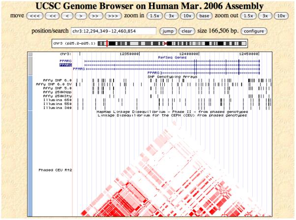
• 7| To capture any upstream regulatory elements we increase the size of the region by adding 10k (arbitrary and depends on the candidate region) at both the start and the end. In the ‘Landmark or Region’ textfield enter ‘chr3:12,294,349-12,460,854’ and press ‘search’ to refresh the view (Figure 2). Under ‘reports and analysis’ choose ‘Download SNP genotype data’ and click on ‘Configure’. In the window that opens up choose ‘CEU’, ‘rs’ and ‘Save to Disk’ and click on “go”. Save the genotype file under a suitable name (here: pparg_dump.txt). This file now contains the genotypes of all SNPs in PPARG +- 10kb that were genotyped in HapMap phase II (Supplementary table 1).

• ▲ Critical step: It has been suggested that the most distal enhancer element is found at a distance of approximately 1 mb from the gene it is regulating. Ensuring to catch such effects within the scope of a standard candidate gene study is likely to involve genotyping a very high number of SNPs. Note that genotypes can also be downloaded using the HapMart facility or bulk downloaded from the FTP server, both accessible from the HapMap webpage.

Figure 2.

View of the candidate genomic region around PPARG using the HapMap genome browser. The plot shows the genotyped SNPs in the region and the different versions of the candidate gene together with other information. The ‘GWA studies (NHGRI Catalog)’ track shows SNPs that have previously been found to be associated with a studied trait in published GWA literature.

Creating a list of functional SNPs to be forced into a tagSNP selection

• 8| The HapMap SNPs are all a subset of the dbSNP database, which can be queried to retrieve information about their functional annotation. The UCSC table browser is a useful tool for retrieving functional annotation from this and other databases. Go to the UCSC genome browser webpage and click on ‘Table browser’. Start with the preset default settings and select ‘group: Variation and Repeats’, ‘tracks: SNPs (129)’ and ‘table: snp129. In the textfield to the right of ‘region:’ enter the interval used in the last step and click on ‘position’. Enter ‘snpAnnotation.txt’ in the ‘output file:’ text field and click on ‘get output’ to save the results (Supplementary table 2).

• ▲ Critical step: There are many publicly available tools for in-depth evaluation of the functional annotation of genetic variants. One useful example is HuGE navigator (http://hugenavigator.net/HuGENavigator/startPageMapper.do), which facilitates interactive searches across databases and interpretation of results by cross-referencing.

• ?Troubleshooting: In the table browser entry page click on ‘describe table schema’ to view a description of the information available in the selected table.

• 9| Open up the file in Excel, sort it by the ‘func’ column, which contains information about the functional annotation, and keep entries which for this column starts with ‘coding’ or ‘cds. Copy the column with the remaining rs names to a text editor. The marker ‘rs1801282’ which has previously been implicated to be associated with type 2 diabetes is added to the list and the filed saved as ‘forceList.txt’ (Supplementary table 3).

• ▲Critical step: The final force list is compiled from the entries in the dbSNP database, which contains many SNPs that might not have been validated or that has not been genotyped in the HapMap project. When later importing the forceList for the selection of tagSNPs, the markers that are not available in the dataset are automatically excluded. The choice of criteria to use for selecting markers differs between studies. Our selection is somewhat arbitrary and was chosen for illustration purposes. More advanced selection, forcing in markers in for example promoters and UTRs, involves more in-depth data analysis of the candidate regions and the elements therein ¹⁸.

Selecting tagSNPs

• 10| Haploview ²² is a popular software for selecting tagSNPs and visualising LD. TagSNPs can be selected by using HaploView through the graphical user interface (GUI) or through a terminal running it in command line mode. Running HaploView with a GUI has many advantages in terms of ease-of-use and display functions. However, when tagging a larger genomic region, it is advisable to use a server where the application can run in the background for computational reasons.

• (A) HaploView with GUI

• (i) Start up Haploview by clicking on the haploview.jar file. In the ‘Welcome to HaploView window’, select the ‘HapMap Format’ tab on the left side. Click the grey ‘browse’ button, and select the SNP genotype file downloaded at step 7: pparg_dump.txt. Leave the options as they are (ignore pairwise comparison of markers > 500kb apart, and exclude individuals with > 50% missing genotypes). Click ‘OK’. After import, the data can be accessed through four tabs. In the ‘LD Plot’ tab the LD structure in the region is interactively visualised, the ‘Haplotypes’ tab shows the predicted haplotypes, ‘Check Markers’ summarises in a table the statistics for the 296 imported SNPs and the ‘Tagger’ tab contains the controls for selecting tagSNPs.

• ?Troubleshooting: Depending on which format the genotype data is saved in it might be necessary to select a different tab when importing the data into Haploview.

• (ii) In the ‘Tagger tab’, load the list of markers to force include that was generated in 9 by clicking on ‘Load Includes’. Click on ‘Run Tagger’ to start the calculation. The results from tagger are summarised under the ‘Results’ tab. The selected tagSNPs are shown in the lower left list that can be saved by clicking on ‘Dump Tags File’. The resulting list of tagSNPs will be utilised as input for the quality control and association testing in the following Nature Protocols (Supplementary table 4).

• ▲ Critical steps: 1) It is recommended to select tagSNPs using the ‘pairwise tagging only’ approach. The alternative, multimarker tagging approach, utilises haplotype structure for more efficient selection of tagSNPs. However, this algorithm requires greater genotyping quality and completeness and may result in loss of statistical power; also, data analysis will need to be haplotype-based..

• 2) If only common SNPs are of interest, it is advisable to set the minor allele frequency of tagSNPs to 0.05 in the ‘Check markers’ window, and click on ‘Rescore markers’.

• 3) The LD cut-off specifies that all SNPs with a maximum pair-wise r² below the limit are automatically included in the selection of tagSNPs; the tagger algorithm picks a minimum set of tagSNPs from the remaining SNPs for maximum coverage. A cut-off of r² = 0.8 gives a similar coverage to that for a typical genomewide association study. For better coverage increase the cut-off, though the extent of improvement is region-specific. In our example applying a cut-off of r² ≥0.9 results in a selection of 50 tagSNPs as compared to 42 applying a cutoff of 0.8.

• (B) Haploview from command line

• (i) Start by opening a terminal in which to the type the commands. On Windows open the command prompt, which is most easily accessed through the start menu by clicking on run and typing cmd. If using Mac OSX go through Applications->Utilities and click on Terminal.app. For Unix/Linux check the documentation for the distribution used.

• (ii) To run the Tagger algorithm type ‘java –jar [path_to/]Haploview.jar –nogui –memory 1800 -hapmap [path_to/]pparg_dump.txt –pairwisetagging –tagrsqcutoff 0.8 –minmaf 0.05 –includetagsfile [path_to/]forceList.txt’ (where [path_to/] is the path from the directory where the command is typed to the directory where the haploview.jar file is stored). The arguments after java –jar specify, in order: the location of the haploview program: that no graphical interface should be created: the amount of memory allocated by the system: path to the HapMap genotypes: apply pairwise tagging: use 0.8 as cut-off for LD (r²): exclude markers with minor allele frequency lower than 0.05 and finally path and filename containing a list with markers to force in. In this example specify the list that was compiled in step 9.

• (iii) After running Tagger two files are created, both with the prefix of the input file and ending with .TAGS or .TEST. The .TEST file contains the identifiers of the markers selected by the tagging algorithm and will be used in the following Nature Protocols (Supplementary table 4).

• ?Troubleshooting: To list the options for Haploview, type ‘java –jar [path_to/]Haploview.jar –h’ in the terminal.

Visualising the tagSNPs in the context of PPARG and regional LD structure

• 11| Start Goldsurfer2 ²³ by clicking on the gs2.jar file or the gs2.exe (only for windows) in the unzipped GsWinExe folder. Gs2 can also be opened from the command line by typing ‘java –jar –Xms64m –Xmx1024m gs2.jar’. The –Xmx argument specifies the maximum amount of memory to be allocated by the system. If bigger datasets are to be analysed this setting can be increased accordingly. Open the dataset by clicking on ‘File’>'Load markers' and choosing ‘HapMap(FTP)’ as input format and specifying file to import by clicking on ‘Browse & import’. The imported markers are summarised in the central table and in the summary plots in the right hand side of the window. To get an overview of the data in a genome browser view, click on the plot tab. Plot summary statistics by clicking on ‘Plot>show/hide summary plots’. Select rare SNPs (maf < 0.05) by clicking on the bar showing markers with maf between 0 and 0.05 in the top right histogram. Right-click in the table and choose ‘exclude’ to remove the markers.

• ?Troubleshooting: If importing genotypes saved from other source than specified in the procedure choose import format accordingly.

• 12| Import information about genes in the region by clicking on ‘Bio’ in the main menu and choosing ‘Parse genes (local)’ > ‘Release 36’. Only one variant of the gene is shown since the reference file is based on the ‘knownCanonical' table in UCSC where redundancies and uncertain gene predictions have been removed. Calculate and show LD by going through ‘Plots’ in the main menu and choosing ‘LD’ > ‘2D’ > ‘Recalculate’ or ‘LD’ > ‘3D’ > ‘Show plot’. To show the 3D view of LD, the SNPs to be visualised need to be selected prior to creating the plot. Adjust which tracks to be displayed in the genome view by right-clicking in the plot and selecting ‘Plot settings’. Hide all tracks except for ucscGenes36.txt, snp marks and LD. The vertical and horizontal bars can be used to navigate the view. To illustrate the selection of tagSNPs and the markers kept from forceList.txt, repeat the import of the dump file and again exclude the markers with maf < 0.05. Select the first dataset again and click on 'Stats>Link to other node' and choose the last imported dataset by double-clicking on it. Select the first dataset and paste rs1801282 in the ‘Name (java regexp)’ text field in the Selection dialog, accessed through the ‘Selection’ menu. For the second dataset, repeat the procedure but paste instead the identifiers for the tagSNPs. Click on the first dataset to view the resulting plot (Figure 3).

Figure 3.

Genomeview from GoldSurfer2 showing the selection of tagSNPs (track 2) in relation to PPARG and all HapMap SNPs with minor allele frequency > 0.05 (track 1). The SNP, rs1801282, previously implicated in type 2 diabetes, is highlighted near the start of the PPARG gene. LD is measured in r².

Troubleshooting

For help on the programs and websites used in this protocol, refer to the relevant websites:

• GoldSurfer2 – http://www.well.ox.ac.uk/gs2/tutorial.html

• HaploView - http://www.broad.mit.edu/haploview/user-manual

• UCSC - http://genome.ucsc.edu/goldenPath/help/hgTracksHelp.html

• HapMap browser - http://www.hapmap.org/gbrowse_help.html

• Estimate-coverage.pl - http://www.well.ox.ac.uk/~carl/gwa/cost-efficiency/

Note that bioinformatics websites are continually subject to change, and therefore their precise functionality and resulting displays may differ from the exact wording in this Protocol.

Timing

Candidate gene study

None of the programmes used take longer than a few minutes to run. Exploring the different websites, and displaying and interpreting the relevant information are the rate-limiting steps.

Genomewide association study

The reference file with the LD measurements is relatively large (650MB) with the downloading time depending on the speed of the Internet connection. With a standard broadband connection, downloading is likely to be finished in a few minutes. To run the estimate-coverage.pl script for a panel with ~ 500k SNPs takes around 15 minutes on a standard desktop computer.

Anticipated results

Visualising genomic information in the candidate gene region (PPARG)

Figure 1 shows the PPARG genomic information displayed using the UCSC database by focussing on the region 40kb up and downstream of the RefSeq track NM_138712 (step 5). The LD structure for the CEU shows that the PPARG gene includes two blocks of high LD that expands approximately to the boundaries of the largest variant of the gene. Given that LD does not extend outside of the gene means that there is no need to increase the main interval within which we select our markers. Furthermore substantial cost reductions can be achieved by selecting tagSNPs from within the two large LD blocks. The SNPs captured by different commercially available panels are highlighted and with some of these designed using a tagging approach, it gives an idea about the result obtained by this approach and shows the applicability to use the genotype data from a GWA panel.

Figure 2 shows the PPARG genomic information displayed using the HapMap Genome Browser (step 6). Multiple types of information can be visualised and downloaded by using the combobox under ‘Reports & Analysis’ and the controls under the plot window. Useful features to look at are copy number variations (CNVs) and results from previously published GWA studies by default presented as separate tracks in the plot. By clicking on the question mark beside the ‘GWA studies (NHGRI Catalog)’ label it is possible to get directly linked to published GWA studies.

Retrieving HapMap SNP genotypes for the PPARG region

The saved HapMap genotype dump file (step 7) contains genotype data for 296 SNPs in 90 individuals (Supplementary table 1).

Creating a list of functional SNPs to be forced into a tagSNP selection

The full list downloaded in step 8 contains 832 SNPs (Supplementary table 2). After filtering, the forceList.txt file (step 9) contains 12 SNPs including the previously implicated SNP, rs1801282 (Supplementary table 3).

Selecting tagSNPs

After tagging using HaploView, a set of 42 tagSNPs (Supplementary table 4) was selected including two SNPs that were force-included (steps 10A(ii) and 10B(iii)). The selection of SNPs in the force list was based on the dbSNP database in which a high proportion of the entries are neither validated nor have been genotyped in the HapMap project. This explains why only two of the 12 SNPs in the list enter into the final selection of tagSNPs.

Visualising the tagSNPs in the context of PPARG and regional LD structure

Figure 3 shows the tagSNP visualisation using GoldSurfer2 (step 12). The upper track with SNP marks shows all common (maf > 5%) HapMap SNPs in the region with rs1801282 highlighted in red. The second SNP track shows the coverage of the selected tagSNPs. The knownCanonical gene table from UCSC is cleaned for false hits and redundancies with the effect that only the suggested functional version of PPARG is visible in the plot. LD is measured in r².

Calculating coverage

The calculated coverage is 0.648, as output by the coverage programme.

References

- 1.Lander ES, Linton LM, Birren B, Nusbaum C, Zody MC, Baldwin J, Devon K, Dewar K, Doyle M, FitzHugh W. Initial sequencing and analysis of the human genome. Nature. 2001;409:860–921. doi: 10.1038/35057062. and others. [DOI] [PubMed] [Google Scholar]
- 2.Zondervan KT, Cardon LR. Designing candidate gene and genome-wide case-control association studies. Nature Protocols. 2007;2:2492–2501. doi: 10.1038/nprot.2007.366. [DOI] [PMC free article] [PubMed] [Google Scholar]
- 3.Kruglyak L, Nickerson DA. Variation is the spice of life. Nat. Genet. 2001;27:234–236. doi: 10.1038/85776. [DOI] [PubMed] [Google Scholar]
- 4.Scherer SW, Lee C, Birney E, Altshuler DM, Eichler EE, Carter NP, Hurles ME, Feuk L. Challenges and standards in integrating surveys of structural variation. Nat. Genet. 2007;39:7–15. doi: 10.1038/ng2093. [DOI] [PMC free article] [PubMed] [Google Scholar]
- 5.Sachidanandam R, Weissman D, Schmidt SC, Kakol JM, Stein LD, Marth G, Sherry S, Mullikin JC, Mortimore BJ, Willey DL. A map of human genome sequence variation containing 1.42 million single nucleotide polymorphisms. Nature. 2001;409:928–933. doi: 10.1038/35057149. and others. [DOI] [PubMed] [Google Scholar]
- 6.Gabriel SB, Schaffner SF, Nguyen H, Moore JM, Roy J, Blumenstiel B, Higgins J, DeFelice M, Lochner A, Faggart M. The structure of haplotype blocks in the human genome. Science. 2002;296:2225–2229. doi: 10.1126/science.1069424. and others. [DOI] [PubMed] [Google Scholar]
- 7.The International HapMap Consortium A haplotype map of the human genome. Nature. 2005;437:1299–1320. doi: 10.1038/nature04226. [DOI] [PMC free article] [PubMed] [Google Scholar]
- 8.Johnson GCL, Esposito L, Barratt BJ, Smith AN, Heward J, Di Genova G, Ueda H, Cordell HJ, Eaves IA, Dudbridge F. Haplotype tagging for the identification of common disease genes. Nat. Genet. 2001;29:233–237. doi: 10.1038/ng1001-233. and others. [DOI] [PubMed] [Google Scholar]
- 9.The International HapMap Consortium A second generation human haplotype map of over 3.1 million SNPs. Nature. 2007;449:851–861. doi: 10.1038/nature06258. [DOI] [PMC free article] [PubMed] [Google Scholar]
- 10.Hirschhorn JN, Lohmueller K, Byrne E, Hirschhorn K. A comprehensive review of genetic association studies. Genet. Med. 2002;4:45–61. doi: 10.1097/00125817-200203000-00002. [DOI] [PubMed] [Google Scholar]
- 11.Kuhn RM, Karolchik D, Zweig AS, Trumbower H, Thomas DJ, Thakkapallayil A, Sugnet CW, Stanke M, Smith KE, Siepel A. The UCSC Genome Browser Database: Update 2007. Nucleic Acids Res. 2007;35:668–673. doi: 10.1093/nar/gkl928. and others. [DOI] [PMC free article] [PubMed] [Google Scholar]
- 12.Evans DE, Barrett JC, Cardon LR. To what extent do scans of non-synonymous SNPs complement denser genome-wide association studies? Eur. J. Hum. Genet. 2008;16:718–23. doi: 10.1038/sj.ejhg.5202011. [DOI] [PubMed] [Google Scholar]
- 13.Perkel J. SNP genotyping: six technologies that keyed a revolution. Nat. Methods. 2008;5:447–453. [Google Scholar]
- 14.Syvanen AC. Toward genome-wide SNP genotyping. Nat. Genet. 2005;37:5–10. doi: 10.1038/ng1558. [DOI] [PubMed] [Google Scholar]
- 15.Kingsmore SF, Lindquist IE, Mudge J, Gessler DD, Beavis WD. Genome-wide association studies: progress and potential for drug discovery and development. Nat. Rev. Drug Discov. 2008;7:221–30. doi: 10.1038/nrd2519. [DOI] [PMC free article] [PubMed] [Google Scholar]
- 16.The Wellcome Trust Case Control Consortium Genome-wide association study of 14,000 cases of seven common diseases and 3,000 shared controls. Nature. 2007;447:661–678. doi: 10.1038/nature05911. [DOI] [PMC free article] [PubMed] [Google Scholar]
- 17.Barrett JC, Cardon LR. Evaluating coverage of genome-wide association studies. Nat. Genet. 2006;38:659–662. doi: 10.1038/ng1801. [DOI] [PubMed] [Google Scholar]
- 18.Birney E, Stamatoyannopoulos JA, Dutta A, Guigo R, Gingeras TR, Margulies EH, Weng ZP, Snyder M, Dermitzakis ET, Stamatoyannopoulos JA. Identification and analysis of functional elements in 1% of the human genome by the ENCODE pilot project. Nature. 2007;447:799–816. doi: 10.1038/nature05874. and others. [DOI] [PMC free article] [PubMed] [Google Scholar]
- 19.Anderson CA, Pettersson FH, Barrett JC, Zhang JJ, Ragoussis J, Cardon LR, Morris AP. Evaluating the effects of imputation on the power, coverage and cost-efficiency of genome-wide SNP platforms. Am. J. Hum. Genet. 2008;83:112–119. doi: 10.1016/j.ajhg.2008.06.008. [DOI] [PMC free article] [PubMed] [Google Scholar]
- 20.Marchini J, Howie B, Myers S, McVean G, Donnelly P. A new multipoint method for genome-wide association studies by imputation of genotypes. Nat. Genet. 2007;39:906–913. doi: 10.1038/ng2088. [DOI] [PubMed] [Google Scholar]
- 21.Altshuler D, Hirschhorn JN, Klannemark M, Lindgren CM, Vohl MC, Nemesh J, Lane CR, Schaffner SF, Bolk S, Brewer C. The common PPAR gamma Pro12Ala polymorphism is associated with decreased risk of type 2 diabetes. Nat. Genet. 2000;26:76–80. doi: 10.1038/79216. and others. [DOI] [PubMed] [Google Scholar]
- 22.Barrett JC, Fry B, Maller J, Daly MJ. Haploview: analysis and visualization of LD and haplotype maps. Bioinformatics. 2005;21:263–265. doi: 10.1093/bioinformatics/bth457. [DOI] [PubMed] [Google Scholar]
- 23.Pettersson F, Morris AP, Barnes MR, Cardon LR. Goldsurfer2 (Gs2): A comprehensive tool for the analysis and visualization of genome wide association studies. BMC Bioinformatics. 2008;9 doi: 10.1186/1471-2105-9-138. [DOI] [PMC free article] [PubMed] [Google Scholar]
Associated Data
This section collects any data citations, data availability statements, or supplementary materials included in this article.