Improving the accuracy of predicting secondary structure for aligned RNA sequences

Abstract

Considerable attention has been focused on predicting the secondary structure for aligned RNA sequences since it is useful not only for improving the limiting accuracy of conventional secondary structure prediction but also for finding non-coding RNAs in genomic sequences. Although there exist many algorithms of predicting secondary structure for aligned RNA sequences, further improvement of the accuracy is still awaited. In this article, toward improving the accuracy, a theoretical classification of state-of-the-art algorithms of predicting secondary structure for aligned RNA sequences is presented. The classification is based on the viewpoint of maximum expected accuracy (MEA), which has been successfully applied in various problems in bioinformatics. The classification reveals several disadvantages of the current algorithms but we propose an improvement of a previously introduced algorithm (CentroidAlifold). Finally, computational experiments strongly support the theoretical classification and indicate that the improved CentroidAlifold substantially outperforms other algorithms.

INTRODUCTION

Prediction of the secondary structure for aligned RNA sequences (which is usually called a ‘common’ or ‘consensus’ secondary structure) is an important problem in many fields of RNA research, including non-coding RNA (1) and viral RNAs (2). The (common) secondary structure is often useful for improving the limiting accuracy of conventional secondary structure prediction [e.g. RNAfold (3) and Mfold (4)]. Moreover, it plays an essential role in phylogenetic analysis of RNAs and gene finding of RNAs from genomic sequences (5–11).

A number of algorithms for common secondary structure prediction have been proposed. A well-known program, RNAalifold (12,13), is based on the free energies of the secondary structures of the RNA sequences in the given alignment (thermodynamic information) and the mutation of two bases that maintain a base pair (bonus of co-variation). RNAalifold has been used in a number of studies e.g. (5,6,9). Recent changes to RNAalifold have improved its performance substantially (12). A probabilistic version of RNAalifold is called RNAalipffold model (12), which gives a probability distribution of common secondary structures of the input alignment. RNAalifold is considered as the maximum likelihood (ML) estimation of RNAalipffold model. Another popular program, Pfold (14), uses stochastic context-free grammars (SCFGs) with the phylogenetic information of the input RNA sequences. Pfold also provides a probability distribution of common secondary structures of the input alignment (we call it Pfold model). Recently, PETfold (15), which employs both the thermodynamic and phylogenetic information, has been proposed. McCaskill-MEA (16) achieved robust prediction of common secondary structure by using the averaged base pairing probability matrix based on a thermodynamic model. Both PETfold and McCaskill-MEA are based on the principle of the maximum expected accuracy (MEA), which maximizes the expected accuracy of a prediction with respect to a probability distribution on the entire set of candidate solutions. Another MEA-based algorithm, CentroidAlifold (17), maximizes the sum of the expected gain (of a carefully designed gain function) under a probability distribution of secondary structures of every RNA sequence in the alignment, where the distribution is given by McCaskill model (18) (energy-based model) or CONTRAfold model (19) (machine learning-based model). The estimator of CentroidAlifold is closely related to the γ-centroid estimator (17), which is employed in CentroidFold (20) for conventional secondary structure prediction. The combination of RNAalipffold model (or Pfold model) with the γ-centroid is called RNAalipffold-Centroid (or Pfold-Centroid) (17).

Recent studies have suggested that the principle of MEA, which is used in PETfold, McCaskill-MEA and CentroidAlifold, gives powerful estimators for estimation problems in bioinformatics, including RNA secondary structure prediction (17,19,21,22), common secondary structure prediction from a multiple alignment of RNA sequences (15,16), pairwise/multiple alignment of biological sequences (23,24,25,26), genome alignment (27), transmembrane topology and signal peptide prediction (28), recombination detection (29), gene prediction (30), RNA–RNA interaction (31) and multiple alignment for structured RNAs (32).

In this study, toward improving the accuracy of previously proposed algorithms, we first classify existing software of common secondary structure prediction. The classification is based on an MEA-based estimator with respect to the evaluation process of the common secondary structure prediction. We then propose an improvement of CentroidAlifold by using a mixture distribution of a probability distribution of common secondary structures (e.g. RNAalifold model or Pfold model) and that of secondary structures of each RNA sequence (e.g. McCaskill model or CONTRAfold model). Finally, we show that the improved CentroidAlifold substantially outperforms other algorithms by performing computational experiments.

MATERIALS AND METHODS

Two evaluation processes for common secondary structure prediction

In the problem of common secondary structure prediction (we do not predict each secondary structure of the sequences in a given alignment but predict one common secondary structure of the alignment), two evaluation processes have been used. The first one is to compare the predicted common secondary structure with a reference (correct) common secondary structure directly (Evaluation Process 1; Supplementary Figure S1). However, this evaluation is not so often used in actual evaluations because the definition of the reference common secondary structure is unclear and it is often difficult to prepare the reference common secondary structure of a given alignment, for example, the alignment produced by aligners such as ClustalW (33) and ProbCons (34). Therefore, another evaluation is often conducted (Evaluation Process 2; Supplementary Figure S2): the (predicted) common secondary structure is mapped to each RNA sequence in the input alignment, and then the mapped secondary structures are compared with the reference secondary structure of each RNA sequence (the reference secondary structure is, e.g. obtained from X-ray crystallography or NMR). In other words, a (common) secondary structure that recovers the secondary structures of each RNA sequence in the alignment is a good prediction. Although we need to prepare the reference secondary structures of each RNA sequence in the input alignment in order to conduct this evaluation, it is much easier than preparing the reference ‘common’ secondary structure, as the reference structure of individual RNA sequence can be obtained by using a database, such as Rfam (35) or RNAstrand (36). It should be noted that, in the both evaluation processes, the comparison between two secondary structures (or common secondary structures) is based on the base pairs that are essential for forming secondary/tertiary structures, which are known to be biologically important. More precisely, the sensitivity (SEN) and positive predictive value (PPV) with respect to base-pairs are commonly used in those evaluations.

MEA-based estimators

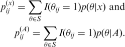
As proposed in (17), two MEA-based estimators (of secondary structure prediction for aligned RNA sequences) that fit with the two evaluation processes can be introduced:

• (E1) the estimator that fits with Evaluation Process 1, which maximizes the expected gain (of a gain function) under a probability distribution of (common) secondary structures of the input alignment (Figure 1);

• (E2) the estimator that fits with Evaluation Process 2, which maximizes the ‘sum’ of the expected gain (of a gain function) under a probability distribution of secondary structures of each RNA sequence in the alignment (Figure 2).

Figure 1.

The MEA-based estimator (E1) with respect to Evaluation Process 1. We assume there exists a probability distribution p(θ|A) of the common secondary structures of the alignment A, and a gain function G(θ, y) between two secondary structure whose length is equal to the length of the alignment (y and θ are considered as the predicted structure and the reference structure, respectively). The gain function characterizes a similarity between the two secondary structures. The estimator is consistent with Evaluation Process 1 (Supplementary Figure S1). See Supplementary Section A.4.1 for details.

Figure 2.

The MEA-based estimator (E2) with respect to Evaluation Process 2. We assume there exists a probability distribution p_x(θ|A) of common secondary structures of x for every x ∈ A and a gain function G(θ, y) between two secondary structure whose length is equal to the length of the alignment (y and θ are considered as the predicted structure and the reference structure, respectively). The estimator is consistent with Evaluation Process 2 (see Supplementary Figure S2). See Section A.4.2 in the supplementary information for details.

In the above estimators, the ‘gain function’ characterizes a similarity between a predicted structure and the reference structure, and should fit with the accuracy measures for the target problems. Also, the probability distributions play an important role in the estimator. Further details of the estimators are shown in Supplementary Section A.4.

Experimental settings

We used a Linux machine with a 2.8 GHz AMD Opteron Processor 854 and 64 GB of memory.

Comparison of methods

In the experiments, we compared the following algorithms or tools: (i) CentroidAlifold (new) (this work), (ii) CentroidAlifold (old) (12), (iii) RNAalifold (updated version of ViennaRNA package 1.8.3) (12), (iv) RNAalifold-Centroid (with the updated version of RNAalifold) (12,17), (v) Pfoldcentroid (14,17) and (vi) PETfold (15). In CentroidAlifold (new/old), we used two probability distributions of secondary structures of a given RNA sequence [i.e. p(θ|x) in Equation (2)]: the McCaskill model in ViennaRNA package 1.8.3 (3) and the CONTRAfold model (Version 2.02) (19). In CentroidAlifold (new), we employed two probability distributions for p(θ|A) in Equation (2): the Pfold model (14) and the RNAalipfold model (12). The weighting was fixed at w = 1/2. We used 17 γ parameters: γ ∈ {2^k : −5 ≤ k ≤ 10, k ∈} ∪ {6} for CentroidAlifold, Pfold-Centroid and RNAalifold-Centroid in order to draw the performance (SEN–PPV) curves.

Data sets

We used the data set of Kiryu et al. (16) that contains 85 multiple alignments and their reference common secondary structures. The number of families in the data set is 17; For each family, there are 5 sub alignments of randomly selected 10 sequences [This data set is the same as in our previous study (17)]. Each item in the data set consists of a manually curated multiple alignment and the reference common secondary structure of the alignment, which were derived from the Rfam database (35,37) and reliable publications. (In other words, the data set does not contain any ‘predictions’ at all.) The reference common secondary structure is used when we conduct Evaluation Process 1. Furthermore, the reference secondary structures of each sequence in the alignment are obtained by mapping the reference common secondary structure to the sequence. These reference structures are used for Evaluation Process 2. We produced several multiple alignments from the same sequences in the reference alignments by using four multiple aligners: ProbCons (34), MAFFT (38), MXSCARNA (39) and ClustalW (33). Those multiple alignments were used in Evaluation Process 2.

RESULTS AND DISCUSSION

Theoretical classification of state-of-the-art algorithms reveals disadvantages of those algorithms

CentroidAlifold (17), RNAalifold (12), Pfold (14), PETfold (15), RNAalifold-Centroid (12,17), Pfold-Centroid (14,17) and McCaskill-MEA (16) can be written as the MEA-based estimator (E2) in Figure 2 with a combination of the gain function G and a probability distribution p_x(θ|A) of secondary structures of x in the input alignment, as follows. [See Table 1; See also Supplementary Section A.5 for more details; Note that the estimator (E1) can be considered as the estimator (E2) as described in Supplementary Section A.4.3.]

Table 1.

All cases are represented in terms of a gain function (G(θ, y)) and a probability distribution of sequence x in the input alignment A(p_x(θ|A)) which are components in the estimator (E2) (Figure 2)

Algorithms	G(θ, y)		px(θ|A)		Ref.
CentroidAlifold (new)	G3		P3	Mixture of p(mcc)(θ|x)/p(contra)(θ|x) and p(alipffold)(θ|A)/p(pfold)(θ|A)	this work
CentroidAlifold (old)	G3		P2	p(mcc)(θ|x) or p(contra)(θ|x)	(16)
McCaskill-MEA	G2		P2	p(mcc)(θ|x)	(26)
PETfold	G2		P3	Mixture of p(mcc)(θ|x) and p(pfold)(θ|A)	(37)
Pfold	G2		P1	p(pfold)(θ|A)	(27)
Pfold-Centroid	G3		P1	p(pfold)(θ|A)	(16,27)
RNAalifold	G1	G(δ)	P1	p(alipffold)(θ|A)	(2)
RNAalipffold-Centroid	G3		P1	p(alipffold)(θ|A)	(2,16)

Algorithms	Disadvantages	S.I.
CentroidAlifold (old)	No use of the information of the input alignment A	Section A.5.1
McCaskill-MEA	Use of ; no use of the information of the input alignment A	Section A.5.7
PETfold	Use of	Section A.5.4
Pfold	Use of	Section A.5.5
Pfold-Centroid	Use of the same distribution px(θ|A) for all x∈A	Section A.5.6
RNAalifold	Use of Gδ (i.e. use of the ML estimator)	Section A.5.2
RNAalipffold-Centroid	Use the same distribution px(θ|A) for all x∈A	Section A.5.3

, G^(δ) and are the gain function used in the γ-centroid estimator (17), the delta function and the gain function used in CONTRAfold (19), respectively. p^(mcc)(θ|x) and p^(contra)(θ|x) are McCaskill model (18) and CONTRAfold model (19), respectively, each of which is a probability distribution of secondary structures of RNA sequence x. p^(alipffold)(θ|A) and p^(pfold)(θ|A) are RNAalipffold model (12) and Pfold model (14), respectively, each of which is a probability distribution of common secondary structures of the alignment A. G1-3 and P1-3 show the types of the gain function and the probability distribution, respectively, and G1, G2, P1 and P2 have drawbacks (see the main text). The disadvantages of each algorithm are shown in the bottom table. For comparison, the improved CentroidAlifold [denoted by ‘CentroidAlifold (new)’], which is introduced in this work, is also shown. The column ‘S.I.’ shows the section in the Supplementary Data.

First, the gain function G is one of the following types:

• (G1) the delta function (denoted by G^(δ)) that returns 1 only when two secondary structures are ‘exactly’ the same;

• (G2) the gain function used in CONTRAfold (19) (denoted by ; See also Supplementary Equation (S10)), which is a sum of the correctly predicted (loop or base pairs) position in the sequence; and

• (G3) the gain function used in the γ-centroid estimator (17) (denoted by ; See also Supplementary Equation (S6)), which is a weighted sum of the number of true-positive base pairs and true-negative base pairs

Second, the probability distribution p_x(θ|A) is one of the following types:

• (P1) a probability distribution of common secondary structures for the input alignment A, RNA alipffold model (12) or Pfold model (14);

• (P2) a probability distribution of secondary structures for individual RNA sequence x, McCaskill model (18) or CONTRAfold model (19); and

• (P3) a mixture of probability distributions of (P1) and (P2).

We emphasize that ‘every’ algorithm in Table 1 [expect for ‘CentroidAlifold (new)’, the proposed algorithm in this study] has drawbacks in the gain function and/or the probability distribution because there are several disadvantages of the gain function (G1) and (G2), and the probability distribution (P1) and (P2) as follows.

The use of the gain function (G1) means that the estimator is closely related to the ML estimator, and a number of recent studies have indicated that the ML estimator does not necessarily give reliable predictions for estimation problems on a high-dimensional discrete space, because there are huge number of suboptimal solutions (40) and it is not optimized for the accuracy measures of the target problem (17). The gain function (G2) has a ‘bias’ to the commonly used accuracy measures of secondary structure prediction, compared to the gain function (G3) (17). More precisely, in (17), Hamada et al. proved

(1)

where A(θ, y) is positive for ‘false’ predictions of base pairs (i.e. false positive and false negative) and C(θ) does not depend on the prediction y. This means that the gain function 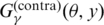has a bias against accurate predictions of base pairs in the secondary structure compared with 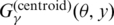, so the estimator with is theoretically superior to the estimator with . See (17) for more detailed descriptions.

The use of the probability distribution (P1) has a disadvantage because the probability distribution is the ‘same’ for each RNA sequence x in the alignment, although it is natural that p_x(θ|A)≠p_x′(θ|A) for x ≠ x′. A drawback of the probability distribution (P2) is that the probability distribution does not employ the information of the input multiple alignment at all. [For example, the probability distribution (P2) does not consider either the covariance bonus or the phylogenetic information of the input alignment.]

These investigations drive us to improve the current CentroidAlifold in the following.

An improvement of CentroidAlifold: theoretically better choice for gain function and probability distributions in MEA-based estimator

In order to overcome the drawbacks of the current state-of-the-art algorithms in Table 1, we employ the MEA-based estimator (E2) with the combination of the gain function (G3) and the probability distribution (P3). Note that there is no algorithm that uses this combination. This means that we replace the probability distribution in CentroidAlifold by a ‘mixture’ of the probability distribution of common secondary structures of A (from the RNAalipffold or Pfold model) and the probability distribution of secondary structures of the individual sequence x in A (from the McCaskill or CONTRAfold model):

(2)

where w ∈ [0, 1] is a weight parameter and p(θ|x) is identical to McCaskill model or CONTRAfold model, and p(θ|A) is identical to RNAalipffold model or Pfold model. Using Equation (2), therefore, means that we consider not only the probability distribution of secondary structures of an individual RNA sequence in A but also the probability distribution of (common) secondary structures of the alignment A. If w = 1, the estimator is equal to that of CentroidAlifold (17) (see also Supplementary Section A.5.1.). On the other hand, if w = 0, the estimator is equivalent to that of RNAalipffold-Centroid or Pfold-Centroid, which are the γ-centroid estimator (17) with the RNAalipffold or Pfold models, respectively (see also Supplementary Section A.5.3 and A.5.6).

The combination of the gain function (G3) and probability distribution (P3) is theoretically better choice than the other combinations, and this will also be confirmed by computational experiments in the following sections.

It should be noted that we used the ‘same’ gain function in both the previous and new CentroidAlifold because the gain function is still thought to be better than any other gain functions [including (G1) and (G2)] for predicting accurate base pairs in (common) secondary structures.

Computation of the improved CentroidAlifold

In the computation of CentroidAlifold, we first compute (n+1) base pairing probability matrices, where n is the number of sequences in A: for x∈A and where

[Here, .] The computational time for this is equal to O(n|A|³) because each base pairing probability matrix can be computed by the Inside-Outside algorithm (41). Finally, CentroidAlifold conducts the following Nussinov-style dynamic programming (DP) recursion (42).

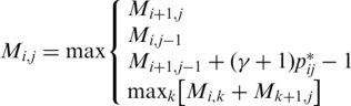(3)

where

(4)

and M_i,j is the optimal score of the subsequence x_i···j. Note that is derived from the mixture distribution of Equation (2). This DP algorithm means that CentroidAlifold maximizes the sum of (base pairing) probabilities of Equation (4) which are larger than 1/(γ + 1). This DP algorithm requires O(|A|³) time and the total computational time of CentroidAlifold still remains O(n|A|³).

Implementation

The improved CentroidAlifold is in the ‘same’ package as CentroidFold (20). The software can employ a mixed distribution given by an arbitrary combination of RNAalipffold, Pfold, McCaskill and CONTRAfold models. The default probability distribution used in CentroidAlifold is an equally weighted mixture of the RNAalipffold and McCaskill model [w = 1/2 in Equation (2)].

Improved CentroidAlifold substantially outperforms other methods in computational experiments

CentroidAlifold (new) clearly outperformed the other algorithms with respect to Evaluation Process 1 for the ‘reference’ alignment (Figure 3). Note that we cannot apply Evaluation Process 1 to the predicted common secondary structure from the multiple alignments produced by the aligners such as ClustalW. This implies that the averaged probability distribution of p_x(θ|A) (i.e. a probability distribution of secondary structures of x) for x ∈ A of CentroidAlifold gives a reliable probability distribution of common secondary structures of A, because, by using the averaged distribution, CentroidAlifold [the estimator (E2)] is considered as the estimator (E1) that is suitable to Evaluation Process 1. (See also Supplementary Section A.4.3.)

Figure 3.

The performance of common secondary structure prediction with the reference alignments with respect to Evaluation Process 1. The horizontal and vertical axes indicate PPV and SEN, respectively. Better performances are in the upper-right areas of each figure (worse performances are to the lower left). The results for the RNAalipffold model are shown on the left and those for the Pfold model on the right. The labels ‘mc’, ‘ct’, ‘pf’ and ‘al’ indicate the McCaskill, CONTRAfold, Pfold and RNAalipffold models, respectively. CentroidAlifold (old: X) indicates CentroidAlifold with probability distribution X (where X = ‘mc’ or ‘ct’). CentroidAlifold (new: Y-X) indicates CentroidAlifold with a mixture of the probability distributions X and Y where Y is p(θ|A), X is p(θ|x) and w = 1/2 in Equation (2) (Y = ‘pf’ or ‘al’). The dashed lines (red/green) show the performance curves of the previous CentroidAlifold, while the solid lines (red/green) show the performance curves of the new CentroidAlifold. In both figures, the performances of PETfold and RNAalifold are also shown.

Moreover, CentroidAlifold (new) outperformed the other algorithms with respect to Evaluation Process 2 (Figure 4 and Supplementary Figures S1–S3). Precisely speaking, CentroidAlifold (new) (the solid lines in red and green colors in each figure) clearly improved the performances of CentroidAlifold (old) (the dashed lines in red and green colors in each figure), and both RNAalipffold-Centroid and Pfold-Centroid (the blue lines), which indicated that the mixing distribution used in CentroidAlifold (new) works very well. Especially, the maximum sensitivity of CentroidAlifold is much better than the one of the other algorithms (Table 2).

Figure 4.

The performance of common secondary structure prediction for Evaluation Process 2 with alignments produced by ProbCons (left column) and the reference alignments (right column). In CentroidAlifold, we used the RNAalipffold model (top row) and the Pfold model (bottom row). See the caption of Figure 3 for notation. Also see Supplementary Figures S1–S3 for the performance with alignments produced by ClustalW (33), MAFFT (38) and MXSCARNA (39), respectively.

Table 2.

The maximum sensitivity for CentroidAlifold (we used a mixture of the probability distributions of the RNAalipffold model and the McCaskill model with the same weight), RNAalipffold-Centroid and Pfold-Centroid in the SEN–PPV curves

Alignment	CentroidAlifold	RNAalipffold-Centroid	Pfold-Centroid
Reference	0.90	0.83	0.81
ClustalW	0.58	0.45	0.44
ProbCons	0.69	0.59	0.58
MAFFT	0.72	0.64	0.64
MXSCARNA	0.75	0.68	0.67

Evaluation Process 2 was used in this experiments. The bold values indicate the best values among three algorithms.

In CentroidAlifold (new), there is few difference of performances between the use of McCaskill model and CONTRAfold model, while the former is about two times as fast as the latter (Table 3). This is because the time for computing the base pairing probability matrix with the CONTRAfold model is longer than for the McCaskill model implemented in the ViennaRNA package. Table 3 also indicates that RNAalifold is the fastest tool because the computational cost of RNAalifold, unlike that of the other tools, does not depend on the number of RNA sequences in the alignments. Moreover, RNAalifold need not use the Inside-Outside algorithm for computing the base pairing probability matrix but can use a Nussinov-type algorithm (42) [cf. Equation (3)] for computing the consistent (common) secondary structure, while CentroidAlifold, PETfold, RNAalipffold-Centroid and Pfold must use both (see ‘Materials and Methods’ section for details). As a result, RNAalifold is more than 10 times faster than the other software and algorithms (Table 3).

Table 3.

Total computational time in seconds

CentroidAlifold
	p (θ|A)	p (θ|x)	time (all)	time (MCC)	time (fixed)
1	pf	ct	1666	1669	1626
2	pf	mc	1239	1247	1200
3	al	ct	932	929	893
4	al	mc	506	500	467
5	pf	–	869	867	832
6	al	–	133	134	99
7	–	ct	837	835	801
8	–	mc	411	410	373
Other software
			Name		Time
9			PETfold		2519
10			RNAalifold		30

The labels ‘pf’, ‘al’, ‘ct’ and ‘mc’ indicate Pfold, RNAalipffold, CONTRAfold and McCaskill models, respectively. p(θ|A) and p(θ|x) are the probability distributions that correspond to the ones in Equation (2). The column ‘time(all)’ means the computational time for computing all the common secondary structures with the 17 γ-parameters of our data-set in order to obtain the SEN-PPV curve after computing the base-pairing probability matrices). The column ‘time(MCC)’ means the computational time for predicting the secondary structure with the pseudo-expected MCC. The column ‘time(fixed)’ means the computational time for computing a secondary structure with a fixed γ. The 5th, 6th, 7th and 8th rows are equivalent to Pfold-Centroid, RNAalipffold-Centroid, CentroidAlifold(old) with the CONTRAfold model and CentroidAlifold(old) with the McCaskill model, respectively.

By the results of our benchmark (Supplementary Table S1), it seems to be enough to use γ = 2 or 4 for obtaining the common secondary structure that achieves a balance between SEN and PPV [i.e. that has a favorable Matthews Correlation Coefficient (MCC)]. Moreover, we tried common secondary structure prediction by combining CentroidAlifold with the ‘pseudo’-expected MCC (M. Hamada, K. Sato and K. Asai, submitted for publication) In the manuscript, we found that the pseudo-expected MCC of a given secondary structure can be computed efficiently (while there is no efficient method to compute the expected MCC) and that the pseudo-expected MCC is a reliable approximation to the expected MCC. By using the pseudo-expected MCC, we are able to select the secondary structure from among the several secondary structures based on 17 values of γ that are used for drawing the performance curves of CentroidAlifold. (Note that we did not use the correct structures for the selection.) Table 4 indicates that the selected common secondary structures achieved better MCC than the structures predicted by PETfold and RNAalifold. On the other hand, Table 3 shows that there was only small computational overhead using the pseudo-expected MCC, compared with the prediction with a fixed γ. This is due to the fact that computing the base pairing probability matrices is the dominant factor in the computational time of CentroidAlifold.

Table 4.

SEN, PPV and MCC for CentroidAlifold, RNAalifold and PETfold with respect to Evaluation Process 2

Alignment	CentroidAlifold			PETfold			RNAalifold
	SEN	PPV	MCC	SEN	PPV	MCC	SEN	PPV	MCC
Reference	0.79	0.88	0.83	0.80	0.80	0.80	0.73	0.82	0.78
ClustalW	0.43	0.65	0.53	0.44	0.59	0.51	0.36	0.67	0.49
ProbCons	0.54	0.79	0.65	0.57	0.66	0.61	0.45	0.75	0.58
MAFFT	0.59	0.75	0.66	0.62	0.66	0.64	0.54	0.72	0.62
MXSCARNA	0.64	0.73	0.68	0.66	0.66	0.66	0.52	0.74	0.62

In CentroidAlifold, we used a mixture of the probability distributions of the RNAalipffold model and the McCaskill model with the same weight, and selected the secondary structure using the pseudo-expected MCC. The bold values indicate the best values among three tools for each accuracy measure.

The computational experiments indicated that a good choice (with respect to accuracy and speed) of the probability distribution p_x(θ|A) in the estimator (E2) is a mixture of the RNAalipffold and the McCaskill model. Also, we have performed the experiments using various parameters of weight [i.e. w in Equation (2)] and confirmed that a weight parameter of around 0.5 in the mixture distribution generally gives a good performance (Figure 5 and Supplementary Figures S6–S10). There is, however, room to do research on the probability distribution (p_x(θ|A) in the estimator (E2) [cf. Equation (S3) in Supplementary Data], because there are a number of possibilities to obtain a better mixture of distributions than the one used in the new CentroidAlifold. For example, we can employ a mixture of three probability distributions [the McCaskill model (18), the Pfold (14) model and the RNAalipffold (12) model], thereby considering the thermodynamic information, the phylogenetic information and the covariance bonus. We can also try the McCaskill model implemented in the software RNAstructure (22) that employs more elaborate energy models than the Vienna RNA package. Finding better combinations of the probability distributions in (P3) is an interesting task.

Figure 5.

The performances of CentroidAlifold with various values of the weight parameter [i.e. w = 0,0.1,0.2, … ,0.9,1 in Equation (2)]. In this experiment, we used the mixture distribution of RNAalipffold model (12) and McCaskill model (18), and the alignments produced by ProbCons (34). The curves with w = 1 and w = 0 are equivalent to the ‘previous’ CentroidAlifold and RNAalipffold-Centroid, respectively. The results of the other combinations of probability distributions and aligners are shown in the Supplementary Data (Supplementary Figures S6–S10).

Comparison of performances among gain functions

The performance of RNAalipffold-Centroid (blue lines in the top figures in Figure 4, Supplementary Figures S1–S3) is slightly better than the performance of RNAalifold (blue points in the top figures in Figure 4, Supplementary Figures S1–S3). This shows that the γ-centroid estimator with the RNAalipffold model (that considers probability distributions of all the secondary structures) is better than the ML estimator with the RNAalipffold model, that is, RNAalifold (that only considers the optimal solution with the highest probability). This result is consistent with the theoretical results: the use of gain function (G3) is better than that of (G1).

On the other hand, CentroidAlifold with the Pfold model and the McCaskill model [‘CentroidAlifold (new; pf-mc)’] is nearly equivalent to PETfold. More precisely, if we substitute the gain function (G3) into (G2) in CentroidAlifold, the estimator is equivalent to the (main part of) PETfold. In Figure 4, it can be seen that ‘CentroidAlifold (new; pf-mc)’ outperforms PETfold. This confirms our theoretical results: the gain function (G2) used in PETfold contains a bias against SEN and PPV, compared with the gain function (G3) used in CentroidAlifold.

Importance of credibility (confidence) limit

Although the proposed estimator employs the entire distributions of (common) secondary structures, it still gives a ‘point’ estimation in a high-dimensional discrete space, and the prediction is ‘uncertain’ (43,44). Therefore, a global measure of uncertainty is important. Fortunately, there exist several studies related to this: the credibility (confidence) limit (43,44), which is the minimum Hamming distance of a hyper-sphere containing a specified fraction of the Boltzmann weighted ensemble. The credibility limit of a common secondary structure predicted by CentroidAlifold can be estimated using a stochastic sampling from the Boltzmann weighted ensemble of the common secondary structure. The stochastic sampling is conducted by a similar method proposed by Ding and Lawrence (45), and it has already been implemented in the software, CentroidAlifold. It should be noted that, if we use the sampling method, the credibility limit can be computed easily. Detailed study about the credibility limit for common secondary structures will be included in our future work.

CONCLUSION

In this study, we systematically discussed state-of-the-art algorithms of predicating secondary structure for aligned RNA sequences, and a classification of those algorithms were presented. Then, we introduced an improvement of CentroidAlifold, which was previously proposed by our group (17). Computational experiments have indicated that the improved CentroidAlifold substantially outperformed the previous one and state-of-the-art algorithms, such as PETfold and RNAalifold. The software is freely available from web site: http://www.ncrna.org/software/centroidalifold, which will be useful for finding non-coding RNAs from genomic sequences or phylogenetic analyses of RNAs.

SUPPLEMENTARY DATA

Supplementary Data is available from NAR online.

FUNDING

‘Functional RNA Project’ of the New Energy Technology Development Organization (NEDO), Grant-in-Aid for Scientific Research on Innovative Areas (in parts). Funding for open access charge: Computational Biology Research Center, National Institute of Advanced Industrial Science and Technology (AIST).

Conflict of interest statement. None declared.

REFERENCES

- 1.Bernhart SH, Hofacker IL. From consensus structure prediction to RNA gene finding. Brief. Funct. Genomic Proteomic. 2009;8:461–471. doi: 10.1093/bfgp/elp043. [DOI] [PubMed] [Google Scholar]
- 2.Schroeder SJ. Advances in RNA structure prediction from sequence: new tools for generating hypotheses about viral RNA structure-function relationships. J. Virol. 2009;83:6326–6334. doi: 10.1128/JVI.00251-09. [DOI] [PMC free article] [PubMed] [Google Scholar]
- 3.Hofacker I, Fontana W, Stadler P, Bonhoeffer S, Tacker M, Schuster P. Fast folding and comparison of RNA secondary structures. Monatsh. Chem. 1994;125:167–188. [Google Scholar]
- 4.Zuker M. Mfold web server for nucleic acid folding and hybridization prediction. Nucleic Acids Res. 2003;31:3406–3415. doi: 10.1093/nar/gkg595. [DOI] [PMC free article] [PubMed] [Google Scholar]
- 5.Clyde K, Harris E. RNA secondary structure in the coding region of dengue virus type 2 directs translation start codon selection and is required for viral replication. J. Virol. 2006;80:2170–2182. doi: 10.1128/JVI.80.5.2170-2182.2006. [DOI] [PMC free article] [PubMed] [Google Scholar]
- 6.Jochl C, Rederstorff M, Hertel J, Stadler PF, Hofacker IL, Schrettl M, Haas H, Huttenhofer A. Small ncRNA transcriptome analysis from Aspergillus fumigatus suggests a novel mechanism for regulation of protein synthesis. Nucleic Acids Res. 2008;36:2677–2689. doi: 10.1093/nar/gkn123. [DOI] [PMC free article] [PubMed] [Google Scholar]
- 7.Okada Y, Sato K, Sakakibara Y. In Proceedings of the 15th Pacific Symposium on Biocomputing. 2010. Improvement of structure conservation index with centroid estimators; pp. 88–97. [DOI] [PubMed] [Google Scholar]
- 8.Stocsits RR, Letsch H, Hertel J, Misof B, Stadler PF. Accurate and efficient reconstruction of deep phylogenies from structured RNAs. Nucleic Acids Res. 2009;37:6184–6193. doi: 10.1093/nar/gkp600. [DOI] [PMC free article] [PubMed] [Google Scholar]
- 9.Thurner C, Witwer C, Hofacker IL, Stadler PF. Conserved RNA secondary structures in Flaviviridae genomes. J. Gen. Virol. 2004;85:1113–1124. doi: 10.1099/vir.0.19462-0. [DOI] [PubMed] [Google Scholar]
- 10.Washietl S, Hofacker IL, Lukasser M, Huttenhofer A, Stadler PF. Mapping of conserved RNA secondary structures predicts thousands of functional noncoding RNAs in the human genome. Nat. Biotechnol. 2005;23:1383–1390. doi: 10.1038/nbt1144. [DOI] [PubMed] [Google Scholar]
- 11.Washietl S, Hofacker IL, Stadler PF. Fast and reliable prediction of noncoding RNAs. Proc. Natl Acad. Sci. USA. 2005;102:2454–2459. doi: 10.1073/pnas.0409169102. [DOI] [PMC free article] [PubMed] [Google Scholar]
- 12.Bernhart S, Hofacker I, Will S, Gruber A, Stadler P. RNAalifold: improved consensus structure prediction for RNA alignments. BMC Bioinformatics. 2008;9:474. doi: 10.1186/1471-2105-9-474. [DOI] [PMC free article] [PubMed] [Google Scholar]
- 13.Hofacker IL, Fekete M, Stadler PF. Secondary structure prediction for aligned RNA sequences. J. Mol. Biol. 2002;319:1059–1066. doi: 10.1016/S0022-2836(02)00308-X. [DOI] [PubMed] [Google Scholar]
- 14.Knudsen B, Hein J. Pfold: RNA secondary structure prediction using stochastic context-free grammars. Nucleic Acids Res. 2003;31:3423–3428. doi: 10.1093/nar/gkg614. [DOI] [PMC free article] [PubMed] [Google Scholar]
- 15.Seemann S, Gorodkin J, Backofen R. Unifying evolutionary and thermodynamic information for RNA folding of multiple alignments. Nucleic Acids Res. 2008;36:6355–6362. doi: 10.1093/nar/gkn544. [DOI] [PMC free article] [PubMed] [Google Scholar]
- 16.Kiryu H, Kin T, Asai K. Robust prediction of consensus secondary structures using averaged base pairing probability matrices. Bioinformatics. 2007;23:434–441. doi: 10.1093/bioinformatics/btl636. [DOI] [PubMed] [Google Scholar]
- 17.Hamada M, Kiryu H, Sato K, Mituyama T, Asai K. Prediction of RNA secondary structure using generalized centroid estimators. Bioinformatics. 2009;25:465–473. doi: 10.1093/bioinformatics/btn601. [DOI] [PubMed] [Google Scholar]
- 18.McCaskill JS. The equilibrium partition function and base pair binding probabilities for RNA secondary structure. Biopolymers. 1990;29:1105–1119. doi: 10.1002/bip.360290621. [DOI] [PubMed] [Google Scholar]
- 19.Do C, Woods D, Batzoglou S. CONTRAfold: RNA secondary structure prediction without physics-based models. Bioinformatics. 2006;22:e90–e98. doi: 10.1093/bioinformatics/btl246. [DOI] [PubMed] [Google Scholar]
- 20.Sato K, Hamada M, Asai K, Mituyama T. CENTROIDFOLD: a web server for RNA secondary structure prediction. Nucleic Acids Res. 2009;37:W277–W280. doi: 10.1093/nar/gkp367. [DOI] [PMC free article] [PubMed] [Google Scholar]
- 21.Hamada M, Sato K, Kiryu H, Mituyama T, Asai K. Predictions of RNA secondary structure by combining homologous sequence information. Bioinformatics. 2009;25:i330–i338. doi: 10.1093/bioinformatics/btp228. [DOI] [PMC free article] [PubMed] [Google Scholar]
- 22.Lu ZJ, Gloor JW, Mathews DH. Improved RNA secondary structure prediction by maximizing expected pair accuracy. RNA. 2009;15:1805–1813. doi: 10.1261/rna.1643609. [DOI] [PMC free article] [PubMed] [Google Scholar]
- 23.Bradley RK, Pachter L, Holmes I. Specific alignment of structured RNA: stochastic grammars and sequence annealing. Bioinformatics. 2008;24:2677–2683. doi: 10.1093/bioinformatics/btn495. [DOI] [PMC free article] [PubMed] [Google Scholar]
- 24.Bradley RK, Roberts A, Smoot M, Juvekar S, Do J, Dewey C, Holmes I, Pachter L. Fast statistical alignment. PLoS Comput. Biol. 2009;5:e1000392. doi: 10.1371/journal.pcbi.1000392. [DOI] [PMC free article] [PubMed] [Google Scholar]
- 25.Holmes I, Durbin R. Dynamic programming alignment accuracy. J. Comput. Biol. 1998;5:493–504. doi: 10.1089/cmb.1998.5.493. [DOI] [PubMed] [Google Scholar]
- 26.Sahraeian SM, Yoon BJ. PicXAA: greedy probabilistic construction of maximum expected accuracy alignment of multiple sequences. Nucleic Acids Res. 2010;38:4917–4928. doi: 10.1093/nar/gkq255. [DOI] [PMC free article] [PubMed] [Google Scholar]
- 27.Frith MC, Hamada M, Horton P. Parameters for accurate genome alignment. BMC Bioinformatics. 2010;11:80. doi: 10.1186/1471-2105-11-80. [DOI] [PMC free article] [PubMed] [Google Scholar]
- 28.Kall L, Krogh A, Sonnhammer EL. An HMM posterior decoder for sequence feature prediction that includes homology information. Bioinformatics. 2005;21(Suppl. 1):i251–i257. doi: 10.1093/bioinformatics/bti1014. [DOI] [PubMed] [Google Scholar]
- 29.Michal N, Tomas V, Brona B. The highest expected reward decoding for hmms with application to recombination detection. arXiv:1001.4499v1. 2010 2010 [Epub ahead of print, 25 Jan 2010] [Google Scholar]
- 30.Gross S, Do C, Sirota M, Batzoglou S. CONTRAST: a discriminative, phylogeny-free approach to multiple informant de novo gene prediction. Genome Biol. 2007;8:R269. doi: 10.1186/gb-2007-8-12-r269. http://genomebiology.com/2007/8/12/R269. [DOI] [PMC free article] [PubMed] [Google Scholar]
- 31.Kato Y, Sato K, Hamada M, Watanabe Y, Asai K, Akutsu T. RactIP: fast accurate prediction of RNA-RNA interaction using integer programming. Bioinformatics. 2009 doi: 10.1093/bioinformatics/btq372. 2009. [DOI] [PMC free article] [PubMed] [Google Scholar]
- 32.Hamada M, Sato K, Kiryu H, Mituyama T, Asai K. CentroidAlign: fast and accurate aligner for structured RNAs by maximizing expected sum-of-pairs score. Bioinformatics. 2009;25:3236–3243. doi: 10.1093/bioinformatics/btp580. [DOI] [PubMed] [Google Scholar]
- 33.Thompson JD, Higgins DG, Gibson TJ. CLUSTAL W: improving the sensitivity of progressive multiple sequence alignment through sequence weighting, position-specific gap penalties and weight matrix choice. Nucleic Acids Res. 1994;22:4673–4680. doi: 10.1093/nar/22.22.4673. [DOI] [PMC free article] [PubMed] [Google Scholar]
- 34.Do C, Mahabhashyam M, Brudno M, Batzoglou S. ProbCons: probabilistic consistency-based multiple sequence alignment. Genome Res. 2005;15:330–340. doi: 10.1101/gr.2821705. [DOI] [PMC free article] [PubMed] [Google Scholar]
- 35.Gardner PP, Daub J, Tate JG, Nawrocki EP, Kolbe DL, Lindgreen S, Wilkinson AC, Finn RD, Griffiths-Jones S, Eddy SR. Rfam: updates to the RNA families database. Nucleic Acids Res. 2009;37:D136–D140. doi: 10.1093/nar/gkn766. [DOI] [PMC free article] [PubMed] [Google Scholar]
- 36.Andronescu M, Bereg V, Hoos H, Condon A. RNA STRAND: the RNA secondary structure and statistical analysis database. BMC Bioinformatics. 2008;9:340. doi: 10.1186/1471-2105-9-340. [DOI] [PMC free article] [PubMed] [Google Scholar]
- 37.Griffiths-Jones S, Moxon S, Marshall M, Khanna A, Eddy SR, Bateman A. Rfam: annotating non-coding RNAs in complete genomes. Nucleic Acids Res. 2005;33(Database issue):121–124. doi: 10.1093/nar/gki081. [DOI] [PMC free article] [PubMed] [Google Scholar]
- 38.Katoh K, Kuma K, Toh H, Miyata T. Mafft version 5: improvement in accuracy of multiple sequence alignment. Nucleic Acids Res. 2005;33:511–518. doi: 10.1093/nar/gki198. [DOI] [PMC free article] [PubMed] [Google Scholar]
- 39.Tabei Y, Kiryu H, Kin T, Asai K. A fast structural multiple alignment method for long RNA sequences. BMC Bioinformatics. 2008;9:33. doi: 10.1186/1471-2105-9-33. [DOI] [PMC free article] [PubMed] [Google Scholar]
- 40.Carvalho L, Lawrence C. Centroid estimation in discrete high-dimensional spaces with applications in biology. Proc. Natl Acad. Sci. USA. 2008;105:3209–3214. doi: 10.1073/pnas.0712329105. [DOI] [PMC free article] [PubMed] [Google Scholar]
- 41.Durbin R, Eddy S, Krogh A, Mitchison G. Biological Sequence Analysis. Cambridge, UK: Cambridge University press; 1998. [Google Scholar]
- 42.Nussinov R, Pieczenk G, Griggs J, Kleitman D. Algorithms for loop matchings. SIAM J. Appl. Math. 1978;35:68–82. [Google Scholar]
- 43.Newberg LA, Lawrence CE. Exact calculation of distributions on integers, with application to sequence alignment. J. Comput. Biol. 2009;16:1–18. doi: 10.1089/cmb.2008.0137. [DOI] [PMC free article] [PubMed] [Google Scholar]
- 44.Webb-Robertson BJ, McCue LA, Lawrence CE. Measuring global credibility with application to local sequence alignment. PLoS Comput. Biol. 2008;4:e1000077. doi: 10.1371/journal.pcbi.1000077. [DOI] [PMC free article] [PubMed] [Google Scholar]
- 45.Ding Y, Lawrence CE. A statistical sampling algorithm for RNA secondary structure prediction. Nucleic Acids Res. 2003;31:7280–7301. doi: 10.1093/nar/gkg938. [DOI] [PMC free article] [PubMed] [Google Scholar]
Associated Data
This section collects any data citations, data availability statements, or supplementary materials included in this article.