Association screening of common and rare genetic variants by penalized regression

Abstract

Motivation: This article extends our recent research on penalized estimation methods in genome-wide association studies to the realm of rare variants.

Results: The new strategy is tested on both simulated and real data. Our findings on breast cancer data replicate previous results and shed light on variant effects within genes.

Availability: Rare variant discovery by group penalized regression is now implemented in the free program Mendel at http://www.genetics.ucla.edu/software/

Contact: huazhou@ucla.edu

Supplementary information: Supplementary data are available at Bioinformatics online.

1 INTRODUCTION

Genome-wide association studies (GWASs) have enjoyed varying degrees of success in the past decade (Easton and Eeles, 2008; Frazer et al., 2009; Lettre and Rioux, 2008). The failure of single nucleotide polymorphism (SNP)-based studies to explain a substantial fraction of trait variation is hardly surprising given the tendency of selection to drive even weakly deleterious mutations to extinction. There are several candidates for the missing dark matter of genetic epidemiology. Among these are: (i) copy number variants (CNVs); (ii) polygenes of small effect; (iii) interactions between genes and between genes and environment; (iv) epigenetic effects; and (v) rare variants. Rare variants are currently attracting the most attention. CNVs are subject to the same selective forces as SNPs. The sole benefit of discovering polygenes of small effect is the insight these provide into biochemical pathways and genetic networks. Detecting interactions is problematic unless they are large or sample sizes are very large. Epigenetic effects and parent-of-origin effects are clearly important in certain settings and deserve more study. In view of the recent striking advances in large-scale sequencing (Hodges et al., 2007), the search for rare variants is apt to be the most promising route to disease gene discovery.

Statistical methods must evolve to meet the challenges of sequence data. Most current analysis methods are predicated on the common disease common variant (CDCV) hypothesis, which postulates that common diseases are caused by common variants of small to modest effect. The competing common disease rare variant (CDRV) hypothesis postulates that common diseases are caused collectively by multiple rare variants of moderate to large effect. Macular degeneration is cited as an example supporting the CDCV hypothesis (RetNet, 2010). Because macular degeneration onset is typically late in life, it has a small impact on Darwinian fitness. The CDRV hypothesis receives support from traits such as low plasma levels of HDL cholesterol (Cohen et al., 2004), cystic fibrosis (Dean and Santis, 1994), colorectal adenomas (Azzopardi et al., 2008), familial breast cancer (Johnson et al., 2007) and schizophrenia (Walsh et al., 2008). The distinction between the two hypotheses is less sharp than proponents might suggest in the heat of argument. There is a spectrum of deleterious allele frequencies within many disease genes, and special circumstances of human history may favor one hypothesis over the other, depending on the diseases and populations studied (Nielsen et al., 2007, 2009).

It makes good statistical sense to consider all predictors (SNP variants and environmental covariates) in concert. Because rare disease predisposing alleles may be present in only a handful of patients, the traditional variant-by-variant approach is doomed to low power. A remedy is to group variants by gene or pathway membership. Once this is done, the strongest marginal signal is assessed by a weighted sum test (Madsen and Browning, 2009) or by a groupwise test exploiting the multivariate and collapsing strategies of Li and Leal (2008). Multiple testing remains a major concern.

The current article extends our recent research on penalized estimation methods in GWAS (Wu et al., 2009) to the realm of rare variants. This approach to association mapping has several advantages: (i) it applies to both ordinary and logistic regression; (ii) it is parsimonious and very fast; (iii) it offers a principled approach to model selection when the number of predictors exceeds the number of study participants; and (iv) it handles interactions gracefully. Our current software relies on lasso penalties and forms part of the Mendel package (Lange et al., 2001). Here, we discuss how to incorporate group penalties that make it easier for related predictors to enter a model once one of the predictors does. For example, one could group all SNPs within a single gene or within several genes in the same pathway. We will argue that a mixture of group penalties and single-predictor penalties tends to work best in practice and constitutes a good alternative to forced collapsing.

When we pass to penalized estimation, model selection is emphasized over hypothesis testing. The lasso penalty is one of the best continuous variable selection mechanisms known for high-dimensional models. The term ‘lasso’ stands for the least absolute shrinkage and selection operator. Unfortunately, the lasso is too stringent for rare variants. Shifting some of the lasso action to a group Euclidean penalty makes it easier for weak or low-frequency predictors to enter a model. Retention of a partial lasso penalty still discourages inclusion of neutral mutations within disease susceptibility genes. The mixed penalty tactic is apt to be most successful when a disease gene harbors a borderline-rare variant with substantial risk. Note that there is no reason to omit common variants in the model selection framework. Hence, a strength of mixed penalties is that they can be applied without choosing between the CDCV and CDRV hypotheses. Once the model selection perspective assumes center stage, multiple testing problems recede. They reappear in replication, but in a more benign form because the number of genes and SNPs of interest drop dramatically.

This niche at the intersection between statistics and genetics is undergoing rapid evolution. Our prior experiences applying lasso-penalized ordinary regression to microarray data (Wu and Lange, 2008) and lasso-penalized logistic regression to GWAS data (Wu et al., 2009) were very encouraging. Since we embarked on the current rare variant research, important work has appeared by a number of authors. The recent technical report of Friedman et al. (2010) introduces a mixture of group and lasso penalties in ordinary regression. Earlier Meier et al. (2008) considered logistic regression with a pure group penalty. Both of these papers fall outside the arena of GWAS. The latter paper also employs different algorithms for optimization. Croiseau and Cordell (2009) applied logistic regression with a pure group penalty to a North American rheumatoid arthritis consortium dataset. However, they treat each SNP as a separate group, whereas we group SNPs by gene or pathway. To our knowledge, there have been no published papers on generalized linear models with mixed group and lasso penalties, certainly none focused on association mapping and rare variants.

The remainder of the article is organized as follows. Section 2 describes our statistical approach and optimization algorithms. It introduces the lasso and group Euclidean penalties, and shows how they can be implemented in linear and logistic regression. The coordinate descent algorithms covered are exceptionally quick and permit optimal tuning of the penalty constant by cross-validation. Section 2 also presents an efficient method for simulating samples under the CDRV model. Section 3 applies the mixed penalty method to two simulation examples. Section 4 analyzes a breast cancer dataset that is small enough to allow comparison to traditional model selection. The discussion highlights some strengths and weaknesses of model selection with mixed penalties and suggests potentially helpful extensions.

2 METHODS

2.1 Lasso and group-penalized regression

Lasso-penalized linear regression (Donoho, 1994; Tibshirani, 1996; Wu and Lange, 2008) is applied to high-dimensional regression problems with tens to hundreds of thousands of predictors. Estimates are derived by minimizing

where y is the response vector, X the design matrix, β the vector of regression coefficients, ‖z‖₂ = (∑_jz_j²)^1/2 the Euclidean (ℓ₂) norm and ‖z‖₁ = ∑_j|z_j| the taxicab (ℓ₁) norm. The sum of squares ‖y − Xβ‖₂² represents the loss function minimized in ordinary least squares; the ℓ₁ contribution ‖β‖₁ is the lasso penalty function. Its multiplier λ > 0 is the penalty constant. The lasso shrinks the estimates of the regression coefficients β_j toward 0. An alternative ridge penalty λ‖β‖₂² also shrinks parameter estimates, but it is not effective in reducing the vast majority of them to 0. For this reason the lasso penalty is preferred to the ridge penalty. Both lasso and ridge regressions are special cases of the bridge regression (Fu, 1998). The constant λ can be tuned to give any desired number of predictors. In this sense, lasso-penalized regression performs continuous model selection. The order predictors enter a model as λ decreases is roughly determined by their impact on the response. Exceptions to this rule occur for correlated predictors.

Logistic regression is handled in a similar manner. Instead of equating the loss function to a sum of squares, we equate it to the negative loglikelihood. The loglikelihood itself can be written as

(1)

where n is the number of responses, θ = (μ, β) the parameter vector and the success probability p_i for trial i is defined by

(2)

Here, the response y_i is 0 (control) or 1 (case), x_i^t the i-th row of the design matrix X and μ an intercept parameter. In practice, statisticians also include the intercept in the ordinary regression model. It can be accommodated by taking the first column of X to be the vector 1 whose entries are identically 1. Because the intercept is felt to belong to any reasonable model, the lasso and ridge penalties omit it. To put the regression coefficients on an equal penalization footing, all predictors should be centered around 0 and scaled to have approximate variance 1. There is a parallel development of lasso-penalized regression for generalized linear models (Park and Hastie, 2007). In each case, the objective function is written as

as the difference between the loglikelihood and the lasso penalty. Because we now maximize f(θ), we subtract the penalty.

In some applications, it is natural to group predictors (Yuan and Lin, 2006). This raises the question of how to penalize a group of parameters. The lasso penalty and the ridge penalties separate parameters. If a parameter enters a model, then it does not strongly inhibit or encourage other associated parameters entering the model. Euclidean penalties have a more subtle effect. Suppose G denotes a group of parameters. Consider the objective function

with a Euclidean penalty on each group. Here, β_G is the subvector of the regression coefficients corresponding to group G. In coordinate ascent, we increase f(θ) by moving one parameter at time. If a slope parameter β_j is parked at 0, when we seek to update it, its potential to move off 0 is determined by the balance between the increase in the loglikelihood and the decrease in the penalty. The directional derivatives of these two functions measure these two opposing forces. The directional derivative of L(θ) is the score for movement to the right and the negative score for movement to the left. An easy calculation shows that the directional derivative of λ‖β_G‖₂ is λ in either direction at β_j = 0 when β_i = 0 for all i ∈ G with i ≠ j. In this case note that ‖β_G‖₂ = |β_j|. If β_G ≠ 0, then the partial derivative of λ‖β_G‖₂ with respect to β_j is λβ_j/|β_G‖₂. Hence, the directional derivatives both vanish at β_j = 0. In other words, the local penalty around 0 for each member of a group relaxes as soon as the regression coefficient for one member moves off 0.

Euclidean group penalties run the risk of selecting response-neutral predictors. As soon as one predictor from a group enters a model, it opens the door for other predictors from the group to enter the model. For this reason, we favor a mixture of group and lasso penalties in ordinary regression. In our genetics context, lasso penalties keep the pressure on for neutral mutations to be excluded, even if they occur in causative genes or pathways. There is no need to group SNPs that occur outside coding or obvious regulatory regions. However, it seems reasonable in the absence of other knowledge to penalize all SNPs equally. This suggests that all Euclidean penalties have the same scale and that the sum of the group and lasso scales for each SNP be the same. Thus, if SNP j belongs to group G, it should experience penalty λ_E‖β_G‖₂+λ_L|β_j|. If it belongs to no group, it should experience penalty λ|β_j| with λ = λ_E+λ_L.

Imposition of lasso and Euclidean penalties has further advantages. In addition to enforcing model parsimony and selecting relevant parameters, both penalties improve the convergence rate in minimizing the objective function. Because the penalties are convex, they also increase the chances for a unique minimum point when the loss function is non-convex. As we demonstrate, both kinds of penalties are compatible with coordinate descent, which is by far the fastest optimization method in sparse regression.

2.2 Algorithms

Coordinate descent/ascent has proved to be an extremely efficient algorithm for fitting penalized models in high-dimensional problems (Friedman et al., 2007; Wu and Lange, 2008; Wu et al., 2009)). Traditional algorithms such as Newton's method and scoring are not computationally competitive. Cyclic coordinate descent/ascent optimizes the objective function one parameter at a time, fixing the remaining parameters. Block relaxation generalizes cyclic coordinate descent by cycling through disjoint blocks of parameters and updating one block at time. Meier et al. (2008) use block relaxation to fit logistic regression. The extreme efficiency of cyclic coordinate descent/ascent in high-dimensional problems stems from the low cost of the univariate updates and the fact that most parameters never budge from their initial value of 0. Here, we present cyclic coordinate descent for linear and logistic regression with mixed lasso and group penalties.

2.2.1 Logistic regression with cases and controls

It is well known that the logistic loglikelihood (1) with success probabilities (2) has score vector and observed information matrix

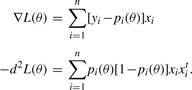For the intercept derivatives, recall that the relevant coordinate of x_i is 1. The penalized loglikelihood augmented by group and lasso penalties becomes

where G ranges over all groups. When λ_L = 0, f(θ) incorporates a pure group penalty (Meier et al., 2008). When λ_E = 0, f(θ) incorporates a pure lasso penalty (Wu et al., 2009).

In penalized maximum likelihood estimation, coordinate ascent is implemented by replacing the loglikelihood by its local quadratic approximation based on the relevant entries of the score and observed information. The penalty contribution is likewise approximated locally by a quadratic in the parameter being updated. For the intercept parameter μ, the penalty can be ignored, and Newton's update amounts to

To update a slope parameter β_j, we commence maximization at 0. If the directional derivatives to the right and left are both negative, then no progress can be made, and β_j remains at 0. Otherwise, maximization is confined to the left or right half-axis, whichever shows promise. Because the objective function is concave, the two directional derivatives cannot be simultaneously positive. If β_j belongs to group G, then the two first two partial derivatives are

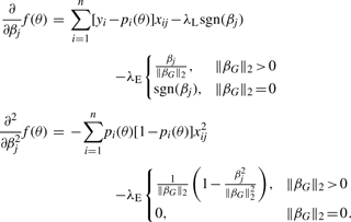The lack of continuity of the first partial derivative at the point β_j = 0 does not prevent the directional derivatives from being well defined. The Newton's update of β_j

(3)

almost always converges within five iterations. At each iteration one should check that the objective function is driven uphill. If the ascent property fails, then the simple remedy of step halving is available.

2.2.2 Ordinary regression with a quantitative trait

The objective function to be minimized is

The Newton update of the intercept is the obvious average

To implement Newton's method for a slope parameter β_j belonging to group G, one employs the first and second partial derivatives

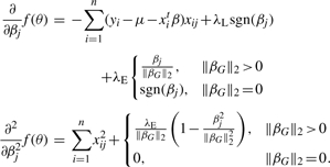With these derivatives in place, the 1D Newton's update (3) is pertinent. Once again iteration is confined to the left or right half-axis, provided either passes the directional derivative test.

2.3 Selection of tuning constants

In principle, cross-validation can be invoked to determine the optimal values of λ_L and λ_E. As we show in our simulations, setting them equal works well. Given a fixed ratio of the two penalties, the total penalty λ = λ_L + λ_E can be adjusted to deliver a predetermined number of genes or SNP variants. Because the number of non-zero predictors entering a model is a generally a decreasing function of λ, a bracketing and bisection strategy is effective in finding a relevant λ (Wu et al., 2009). Of course, the smaller the number of predictors desired, the faster the overall computation proceeds. If computing time is not a constraint, it is helpful to optimize the objective function over a grid of points and monitor how new predictors enter the model as λ decreases.

2.4 Simulation algorithms

For the sake of simplicity, we adopt the rare variant model of Li and Leal (2008). They postulate that any of v variants can independently cause the disease under consideration. If I_i is the indicator of disease attributed to variant i, then the sum S = ∑_i=1^v I_i captures the essence of the model. An individual is affected if and only if his/her value of S satisfies S ≥ 1. Thus, an individual could have multiple mutations, each one sufficient to cause the disease. Ignoring genetic details for the moment, let k_i = Pr(I_i = 1). These prevalences plus the independence of the indicators I_i completely determine the Poisson-binomial distribution characterizing S. The discrete density of S can be computed recursively from the probabilities k_i (Lange, 2010). Once the discrete density is available, we sample from the conditional distribution Pr(S = j ∣ S ≥ 1). Obviously, all I_i = 0 whenever S = 0. Finally, given a positive value j of S, one can sample from the conditional Poisson-binomial

in an efficient sequential manner (Lange, 2010). This brief account omits many details that are fully supplied in the cited reference and the table labeled Algorithm 1.

The most suspect assumption in the model is the independence of the disease indicators I_i, which rules out linkage disequilibrium for closely spaced variants. The remaining genetics assumptions are more defensible. Let G_i be the genotype at variant i. Designate the normal allele by a_i and the high-risk allele by A_i. If the latter has frequency p_i, then under Hardy-−Weinberg equilibrium the three genotypes a_i/a_i = 0, A_i/a_i = 1 and A_i/A_i = 2 have frequencies (1 − p_i)², 2p_i(1 − p_i) and p_i², respectively. Denote the penetrance of the genotype G_i = j at variant i by f_ij = Pr(I_i = 1 ∣ G_i = j). The prevalence attributed to variant i amounts to k_i = ∑_j Pr(G_i = j)f_ij. Under an additive model, . For a multiplicative model, f_i1² = f_i0f_i2. A dominant model takes f_i1 = f_i2, and a recessive model takes f_i0 = f_i1. For purposes of discussion, the wild-type penetrance f₀ = 1 − ∏_i=1^v(1 − f_i0) is the probability that a person with no high-risk alleles is affected. The variant-specific relative risks (RRs) are defined by the ratios γ_ij = f_ij/f₀.

To simulate genotypes in a case/control study, we first simulate the disease indicators I_i, assuming case status (S ≥ 1) or control status (S = 0). Conditional on the indicators I_i, the genotypes G_i are independent. Sampling G_i given I_i is a simple application of Bayes rule taking into account the various genotype probabilities and penetrances. Our entire simulation scheme is summarized in Algorithm 1. Computation of the discrete density of S requires v²/2 operations but only needs to be done once. Simulating each case requires 3v operations and each control v operations. It takes <2 s on a standard laptop to simulate 10000 SNPs for 500 cases and 500 controls.

3 ANALYSIS OF SIMULATED DATA

Our first simulation example compares mixed group and lasso penalties to pure lasso and pure group penalties in association testing. Figure 1 shows the solution paths of a simulation example with 500 cases and 500 controls at various mixes of lasso and group penalties for three genes. Gene 1 (red) contains one common causal variant [minor allele frequency (MAF) 10% and RR 1.2] and four neutral rare variants. Gene 2 (green) contains five causal rare variants (MAF 1% and RR 5) and five neutral rare variants. Gene 3 (blue) contains 10 neutral rare variants. All neutral rare variants have MAF 1% and RR 1. The wild-type penetrance f₀ is set at 0.01. The pure lasso penalty (λ_L/λ = 1) picks up significant variants (common and rare) sequentially. The pure group penalty (λ_L/λ = 0) picks up genes (groups) 1, 2 and 3 sequentially. The mixed group plus lasso penalty (λ_L/λ = 0.75 or 0.50) achieves a good compromise between the two.

Fig. 1.

A simulation example with 500 cases and 500 controls. There are three genes. Gene 1 (red) contains one common causal variant (MAF 10% and RR 1.2) and four neutral rare variants. Gene 2 (green) contains five causal rare variants (MAF 1% and RR 5) and five neutral rare variants. Gene 3 (blue) contains 10 neutral rare variants. All neutral rare variants have MAF 1% and RR 1. The wild-type penetrance f₀ is set at 0.01. The pure lasso penalty (λ_L/λ = 1) picks up significant variants (common and rare) sequentially. The pure group penalty (λ_L/λ = 0) picks up the genes (groups) 1, 2 and 3 sequentially. The mixed group plus lasso penalty (λ_L/λ = 0.75 or 0.50) achieves a good compromise between the two.

Our second simulation example involves 100 simulations each with 500 controls and 500 cases under different scenarios, reflecting heterogeneity in both MAFs and RRs. There are 10 participating

genes, each with 5 rare variants. Across the simulations, the MAF is uniformly distributed from 0.1% to 1%. For i = 1,…, 5, gene i has i causal rare variants. Therefore, the model has 15 causal rare variants dispersed over 5 genes and 35 neutral rare variants dispersed over 10 genes. All neutral variants have RR 1. The wild-type penetrance f₀ is set at 0.01. Figure 2 reports the receiver operating characteristic (ROC) curves calculated from selected variants and genes, with the proportion of the lasso penalty λ_L/λ set at 0 (pure group penalty), 0.5 and 1.0 (pure lasso penalty). Each point of the ROC curves records the true and false positive rates of the selected variants (first row) or genes (second row) at a specific λ value. Inspection of these graphs shows that the performance of the mixed group and lasso penalties dominates that of the pure lasso penalty in variant selection. Note how the green ROC curves are shifted toward the upper left. The effects on gene selection is not clear-cut. The second and third scenarios (columns) support our contention that penalized regression with mixed penalties performs better when any of the causal variants is relatively common or has a high RR in groups.

Fig. 2.

ROC curves based on 100 simulations each with 500 controls and 500 cases. The first row is for variants and the second row for genes. MAFs of all variants are uniform between 0.1% and 1%. Neutral variants have RR 1. Column 1: RRs of causal variants are uniform between 1.2 and 5. Column 2: RRs of causal variants are uniform between 1.1 and 2, except one RR is set to 10 in each causal gene. Column 3: MAF of one variant is set to 5% in each causal gene. The true positive rate (sensitivity) is the proportion of causal variants/genes correctly identified, while the false positive rate (1-specificity) is the proportion of neutral variants/genes identified as causal.

4 APPLICATION TO FAMILY CANCER REGISTRY DATA

Germline mutations in genes from various DNA repair pathways, most notably BRCA1, BRCA2 and ATM, have been shown to dramatically increase the risk of familial breast cancer but do not explain all of the risk (Claus et al., 1996; Ford et al., 1994; Gatti, 1998; Wooster et al., 1995). Based on a candidate gene study of the double-strand break repair (DSBR) pathway, we have identified SNPs from genes involved in DSBR (XRCC4, XRCC2, NBS1, RAD21, TP53, BRIP1, ZNF350) that are associated with risk of familial breast cancer in single SNP analyses (Sehl et al., 2009). Identifying group effects from this pathway can be helpful in understanding factors that modulate an individual's risk of developing breast cancer. We wish to identify group effects by gene and apply here mixed group and lasso-penalized regression.

Family Cancer Registry: data are taken from genotype samples of participants enrolled in the UCLA Family Cancer registry. To be eligible, individuals must have a personal or family history of either a known cancer genetic susceptibility, such as a mutation in BRCA1 or BRCA2, or a family history containing at least two first or second degree relatives who are afflicted with the same primary cancer. This enriched sample of participants allows for the identification of factors that modulate risk of breast cancer. Data analysis has to be fairly subtle because of the way in which the participants were enrolled.

Analysis: we performed penalized logistic regression with the dependent variable, breast cancer status (affected versus unaffected) coded as a binary outcome. We limited our sample to 399 Caucasian participants because other ethnic groups were too small to fully characterize and provide little power to detect differences. There were 196 affected and 203 unaffected individuals. Age was used as a covariate in our analysis. The well-known association of age with breast cancer was confirmed in our previous analysis (Sehl et al., 2009). We imputed missing data for covariates using the mean value for continuous variables and the most frequent category for categorical variables.

SNPs were excluded from our analysis if genotype call rates were <75%. Missing SNPs were imputed using the SNP imputation option of the Mendel 10.0 software (Lange et al., 2001). 148 SNPs from the DSBR pathway were grouped by gene. These 17 genes included BRCA1, BRCA2, BRIP1, ATM, RAD50, RAD51, RAD52, RAD54L, RAD21, TP53, NBS1, XRCC2, XRCC4, XRCC5, MRE11A, ZNF350 and LIG4. Some genes carried large numbers of SNPs (e.g. BRCA2 had 19 SNPs), and some genes had only one SNP for analysis. SNPs were analyzed under additive models. Penalized regression was performed under varying proportions of lasso and group penalties. Analysis under a dominant model leads to similar conclusions (data not shown).

Results: although most of the SNPs in this dataset are common, 4 have MAFs <1%, 5 have MAF between 1% and 5% and 13 have MAF between 5% and 10%. Figure 3 plots the selection trajectories for groups of SNPs and demonstrate the ability of mixed group and lasso-penalized regression to select SNPs within a gene as a group. As the total penalty grows, SNPs are selected either singly or as groups. In the case of the pure lasso, SNPs enter the model singly, and in the case of the pure group penalty, genes enter the model with their full sets of SNPs. In the mixed cases, we see that either single SNPs or sets of SNPs grouped by gene enter the model. When a group enters in the mixed cases, it need not contain all of the SNPs in that gene.

Fig. 3.

SNPs and genes from the DSBR pathway selected by group lasso penalized regression based on familial breast cancer data. All results assume an additive model. Panels reveal the varying trajectories of SNP and gene entrances into the model under varying proportions of lasso to total (lasso plus group) penalty.

Age was the first predictor selected in all models as expected. The content and order of selection of the top four gene-defined groups under varying proportions of lasso to total penalty are shown in Table 1. Under a purely lasso penalty, single SNPs from genes BRIP1, RAD21, RAD52 and XRCC4 are selected. As we increase the proportion of the group penalty, more SNPs from each of these four genes are selected together as a group.

Table 1.

Top four groups of SNPs selected under varying lasso and group penalties and an additive model

λL/λ	Seconda	Thirda	Fourtha	Fiftha
1	BRIP1	XRCC4	RAD21	RAD52
	rs4986763	rs1120476	rs16889040	rs9634161
0.75	RAD21	XRCC4	BRIP1	RAD52
	rs16888927	rs10474081	rs4986763	rs11571476
	rs16888997	rs1120476		rs9634161
	rs16889040	rs6452525		rs7311151
		rs10514249
0.25 – 0.5	XRCC4	RAD21	RAD52b	BRIP1b
	rs10474081	rs16888927	rs11571476	rs4986763
	rs1120476	rs16888997	rs9634161
	rs6452525	rs16889040	rs7311151
	rs10514249
	rs1193695
0c	BRIP1	XRCC4b	RAD21b	RAD52

^aOrder of entry of groups of predictors (following age) into the model.

^bThese groups entered together.

^cFor the pure group penalty results, all SNPs from a gene were selected together; hence individual SNPs are not listed. Values of the total λ required to select the top five predictors are 6.4, 8.6, 10.2 and 10.4 for λ_L/λ equal to 0, 0.25-0.5, 0.75 and 1.0, respectively. The SNPs with P < 0.05 in marginal analysis are boldfaced.

It is reassuring that a broad range of proportions (0.25–0.75) of the lasso penalty deliver stable results. In most models, the same 3 SNPs from RAD21, and the same 4–5 SNPs from XRCC4 are retained. The 3 SNPs from RAD21 lie in a common haplotype block as defined by Gabriel et al. (2002), while the XRCC4 SNPs fall in different haplotype blocks. Many of these SNPs are found to be associated with familial breast cancer in single SNP analyses. In marginal analysis, 14 SNPs have P < 0.05. Ten of these are also selected by the mixed penalty method with λ_L/λ = 0.25 − 0.5 (boldfaced in Table 1). It seems biologically reasonable that these SNP sets should be among the first predictors selected after age.

SNP rs4986763 from gene BRIP1 is present in all models. This SNP was found to be significant in previous single SNP analyses. However, it was only highly significant after excluding individuals who were known to be BRCA1 and BRCA2 positive. RAD52 was not found to be significant in previous single SNP analyses (Sehl et al., 2009), suggesting it may modulate the effects of other SNPs. In a follow-up study (Sehl,M. et al., in preparation), possible interaction of RAD52 with other genes is investigated.

5 DISCUSSION

The results of this article suggest that mixed group and lasso penalties outperform lasso penalties alone, especially when both common and rare variants are present. Our simulated examples clearly demonstrate this fact. Our analysis of the breast cancer data is more ambiguous because we do not know the truth that nature hides. In our view, the focus in genetic epidemiology should be on both SNP and gene discovery.

The connections between penalized regression and Bayesian analysis are obvious. One could argue the case for passing to a full Bayesian assault on association testing. This has already been accomplished for marginal analysis of SNPs (Wellcome Trust Case-Control Consortium, 2007). Although it is tempting to construct multi-predictor Bayesian methods, the computational costs are apt to be high. Penalized estimation and model selection achieve many of the same goals at a fraction of the computational cost.

Mixed penalties help us sort through the confusion of causal genes and neutral variants within them. Even though mixed penalties improve both false positive and false negative rates, we are not suggesting that mixed penalties are a panacea. However, the gradual accumulation of incremental improvements in statistical methods will make a substantial difference. The statistical tools showcased here form part of the next release of the Mendel statistical genetics package. Mendel is available for free in Linux, MacOS and Windows versions at http://www.genetics.ucla.edu/software. It takes <5 s on a standard desktop computer to complete all single SNP analyses and lasso estimation on the family cancer registry data. Our companion paper (Zhou,H. et al., unpublished data) discusses Mendel syntax and output conventions. Geneticists and statisticians wanting to judge for themselves the virtues of mixed penalties are welcome to use Mendel on their own data.

REFERENCES

- Azzopardi D, et al. Multiple rare nonsynonymous variants in the adenomatous polyposis coli gene predispose to colorectal adenomas. Cancer Res. 2008;68:358–363. doi: 10.1158/0008-5472.CAN-07-5733. [DOI] [PubMed] [Google Scholar]
- Claus EB, et al. The genetic attributable risk of breast and ovarian cancer. Cancer. 1996;77:2318–2324. doi: 10.1002/(SICI)1097-0142(19960601)77:11<2318::AID-CNCR21>3.0.CO;2-Z. [DOI] [PubMed] [Google Scholar]
- Cohen JC, et al. Multiple rare alleles contribute to low plasma levels of HDL cholesterol. Science. 2004;305:869–872. doi: 10.1126/science.1099870. [DOI] [PubMed] [Google Scholar]
- Croiseau P, Cordell H. Analysis of North American rheumatoid arthritis consortium data using a penalized logistic regression approach. BMC Proc. 2009;3(Suppl. 7):S61. doi: 10.1186/1753-6561-3-s7-s61. [DOI] [PMC free article] [PubMed] [Google Scholar]
- Dean M, Santis G. Heterogeneity in the severity of cystic fibrosis and the role of CFTR gene mutations. Hum. Genet. 1994;93:364–368. doi: 10.1007/BF00201659. [DOI] [PubMed] [Google Scholar]
- Donoho D, Johnstone I. Ideal spatial adaptation by wavelet shrinkage. Biometrika. 1994;81:425–455. [Google Scholar]
- Easton DF, Eeles RA. Genome-wide association studies in cancer. Hum. Mol. Genet. 2008;17 doi: 10.1093/hmg/ddn287. ddn287+ [DOI] [PubMed] [Google Scholar]
- Ford D, et al. Risks of cancer in BRCA1-mutation carriers. The Lancet. 1994;343:692–695. doi: 10.1016/s0140-6736(94)91578-4. [DOI] [PubMed] [Google Scholar]
- Frazer KA, et al. Human genetic variation and its contribution to complex traits. Nat. Rev. Genet. 2009;10:241–251. doi: 10.1038/nrg2554. [DOI] [PubMed] [Google Scholar]
- Friedman J, et al. Pathwise coordinate optimization. Ann. Appl. Stat. 2007;1:302–332. [Google Scholar]
- Friedman J, et al. A note on the group lasso and a sparse group lasso. 2010 Available at http://www-stat.stanford.edu/∼tibs/ftp/sparse-grlasso.pdf(last accessed date August 16, 2010) [Google Scholar]
- Fu WJ. Penalized regressions: the bridge versus the lasso. J. Comput. Graph. Stat. 1998;7:397–416. [Google Scholar]
- Gabriel SB, et al. The structure of haplotype blocks in the human genome. Science. 2002;296:2225–2229. doi: 10.1126/science.1069424. [DOI] [PubMed] [Google Scholar]
- Gatti RA. Ataxia-telangiectasia. In: Vogelstein B, Kinzler KW, editors. The Genetic Basis of Human Cancer. New York: McGraw-Hill, Inc.; 1998. pp. 275–300. [Google Scholar]
- Hodges E, et al. Genome-wide in situ exon capture for selective resequencing. Nat. Genet. 2007;39:1522–1527. doi: 10.1038/ng.2007.42. [DOI] [PubMed] [Google Scholar]
- Johnson N, et al. Counting potentially functional variants in BRCA1, BRCA2 and ATM predicts breast cancer susceptibility. Hum. Mol. Genet. 2007;16:1051–1057. doi: 10.1093/hmg/ddm050. [DOI] [PubMed] [Google Scholar]
- Lange K, et al. Mendel version 4.0: a complete package for the exact genetic analysis of discrete traits in pedigree and population data sets. Am. J. Hum. Genet. 2001;69(Suppl.):504. [Google Scholar]
- Lange K. Numerical Analysis for Statisticians. 2. New York: Springer; 2010. [Google Scholar]
- Lettre G, Rioux JD. Autoimmune diseases: insights from genome-wide association studies. Hum. Mol. Genet. 2008;17 doi: 10.1093/hmg/ddn246. ddn246+ [DOI] [PMC free article] [PubMed] [Google Scholar]
- Li B, Leal S.MM. Methods for detecting associations with rare variants for common diseases: application to analysis of sequence data. Am. J. Hum. Genet. 2008;83:311–321. doi: 10.1016/j.ajhg.2008.06.024. [DOI] [PMC free article] [PubMed] [Google Scholar]
- Madsen BE, Browning SR. A groupwise association test for rare mutations using a weighted sum statistic. PLoS Genet. 2009;5:e1000384. doi: 10.1371/journal.pgen.1000384. [DOI] [PMC free article] [PubMed] [Google Scholar]
- Meier L, et al. The group Lasso for logistic regression. J. R. Stat. Soc. Series B Stat. Methodol. 2008;70:53–71. [Google Scholar]
- Nielsen R, et al. Recent and ongoing selection in the human genome. Nat. Rev. Genet. 2007;8:857–868. doi: 10.1038/nrg2187. [DOI] [PMC free article] [PubMed] [Google Scholar]
- Nielsen R, et al. Darwinian and demographic forces affecting human protein coding genes. Genome Res. 2009;19:838–849. doi: 10.1101/gr.088336.108. [DOI] [PMC free article] [PubMed] [Google Scholar]
- Park MY, Hastie T. L1-regularization path algorithm for generalized linear models. J. R. Stat. Soc. Series B Stat. Methodol. 2007;69:659–677. [Google Scholar]
- RetNet. 2010. [last accessed date August 16, 2010]. Available at http://www.sph.uth.tmc.edu/retnet. [Google Scholar]
- Sehl ME, et al. Associations between single nucleotide polymorphisms in double-stranded DNA repair pathway genes and familial breast cancer. Clin. Cancer Res. 2009;15:2192–2203. doi: 10.1158/1078-0432.CCR-08-1417. [DOI] [PMC free article] [PubMed] [Google Scholar]
- Tibshirani R. Regression shrinkage and selection via the lasso. J. R. Stat. Soc. Ser. B. 1996;58:267–288. [Google Scholar]
- Walsh T, et al. Rare structural variants disrupt multiple genes in neurodevelopmental pathways in Schizophrenia. Science. 2008;320:539–543. doi: 10.1126/science.1155174. [DOI] [PubMed] [Google Scholar]
- Wellcome Trust Case-Control Consortium. Genome-wide association study of 14,000 cases of seven common diseases and 3,000 shared controls. Nature. 2007;447:661–668. doi: 10.1038/nature05911. [DOI] [PMC free article] [PubMed] [Google Scholar]
- Wooster R, et al. Identification of the breast cancer susceptibility gene BRCA2. Nature. 1998;378:789–792. doi: 10.1038/378789a0. [DOI] [PubMed] [Google Scholar]
- Wu TT, et al. Genome-wide association analysis by lasso penalized logistic regression. Bioinformatics. 2009;25:714–721. doi: 10.1093/bioinformatics/btp041. [DOI] [PMC free article] [PubMed] [Google Scholar]
- Wu TT, Lange K. Coordinate descent algorithms for lasso penalized regression. Ann. Appl. Stat. 2008;2:224–244. [Google Scholar]
- Yuan M, Lin Y. Model selection and estimation in regression with grouped variables. J. R. Stat. Soc. Series B Stat. Methodol. 2006;68:49–67. [Google Scholar]