Automated construction and analysis of the design space for biochemical systems

Abstract

Motivation: Our recent work introduced a generic method to construct the design space of biochemical systems: a representation of the relationships between system parameters, environmental variables and phenotypic behavior. In design space, the qualitatively distinct phenotypes of a biochemical system can be identified, counted, analyzed and compared. Boundaries in design space indicate a transition between phenotypic behaviors and can be used to measure a system's tolerance to large changes in parameters. Moreover, the relative size and arrangement of such phenotypic regions can suggest or confirm global properties of the system.

Results: Our work here demonstrates that the construction and analysis of design space can be automated. We present a formal description of design space and a detailed explanation of its construction. We also extend the notion to include variable kinetic orders. We describe algorithms that automate common steps of design space construction and analysis, introduce new analyses that are made possible by such automation and discuss challenges of implementation and scaling. In the end, we demonstrate the techniques using software we have created.

Availability: The Design Space Toolbox for MATLAB is freely available at http://www.bme.ucdavis.edu/savageaulab/

Contact: masavageau@ucdavis.edu

1 INTRODUCTION

We are awash in a sea of genomic data. Since DNA sequencing was first introduced (Sanger et al., 1977), we have witnessed the sequencing of the entire human genome (Lander et al., 2001; Venter et al., 2001) and over one thousand prokaryotic genomes (NCBI). Thanks to next-generation sequencing technologies (Metzker, 2010; Shendure and Ji, 2008), expectations have grown and audacious efforts are underway to sequence one thousand individual human genomes, one thousand plant genomes and ten thousand vertebrate genomes (1000 Genomes, 1KP and Genome 10K projects). Despite the flood of genomic data, a major unsolved problem remains: relating the known genotypes to phenotypes.

Even at the level of biochemical systems, drawing a connection between genotypic data and system behavior is difficult. First, we must represent the genotypic data with a model, a challenging task in itself. Then, assuming an adequate model exists, its phenotypic responses must be characterized. Because the parameters of the model usually vary, as with environmental change or parameter uncertainty, a direct approach would be to empirically sample many parameter combinations and observe the resulting model behavior. However, the size of the task can quickly grow unreasonable. For example, 10 parameters, each sampled at 20 points, imply an astronomical 10²⁰ trials, and could still miss a point of interest. Furthermore, classification of the behavior is arbitrary. Each trial may exhibit a slightly different phenotype, but without guidance for what constitutes a significant change. To address the issues, our recent work has demonstrated the generic construction of a system design space that represents the relationship between system parameters, environmental variables and phenotypic behavior (Savageau et al., 2009). Boundaries in design space are mathematically defined, based on inherent properties of the model, and naturally separate qualitatively distinct phenotypes of the system, allowing them to be counted and compared. The approach has been successfully applied to various biochemical systems of interest (Coelho et al., 2009; Savageau and Fasani, 2009; Savageau et al., 2009).

Nevertheless, the process of constructing design space has largely been explained by example. Here, we present a formal description of design space and its construction. For the first time, we extend the notion to include variable kinetic orders. We then describe algorithms to automatically construct design space and perform common analyses in the context of design space. We also describe new analyses that are made possible by such automation. Throughout the description, we discuss challenges of implementation and scaling to larger systems. In the end, we present an implementation of the algorithms in software, the Design Space Toolbox for MATLAB, and demonstrate the software with abstract and biological examples.

2 BACKGROUND

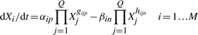
Models of biochemical systems are typically expressed as equations involving mass action or rational functions, which can be recast as generalized mass action (GMA) equations of the form

(1)

where the change in a concentration of interest, X_i, is described by a nonlinear ordinary differential equation. Rate constants appear as the coefficients α_ik and β_ik, and kinetic orders as the exponents g_ijk and h_ijk. The i-th equation contains P_i positive terms and N_i negative terms. Overall, there are M equations and Q concentrations, some of which can vary independently.

The concentrations and rate constants are limited to positive real numbers and, in traditional chemical kinetics, the kinetic orders are limited to small integer values, such as 1 or 2. However, in the power-law formalism (Savageau, 2001, 2009), kinetic orders are allowed to take on real, non-integer values, giving rise to the GMA form. As such, traditional rate law models are a subset of, and can be represented by, GMA models. Furthermore, biochemical kinetics are typically described by rational functions, as in Michaelis–Menten kinetics. However, it has been shown that via a process of recasting (Savageau, 2001; Savageau and Voit, 1987), such systems can be exactly represented by an equivalent GMA system. Hence, the GMA form can be used to represent most models of interest and serves as the basis for the design space methodology.

2.1 The dominant S-system

We are particularly interested in the steady states of the model, or the solutions of the nonlinear system described by Equation (1) when the rates of change equal zero. However, to find every solution of a particular system is typically difficult, to do so for every combination of parameters exceedingly so. Instead, we consider an approximation: assuming one positive term and one negative term dominate the others in each equation—or, biochemically speaking, two reactions exceed the others—the model can be approximated by an S-system, which has a single analytic steady state solution that is linear in the logarithm of the independent concentrations and rate constants (Savageau et al., 2009). The dominant S-system can be described by

(2)

where p and n are the indices of the dominant positive term and the dominant negative term, respectively. At steady state, the equations can be rearranged and logarithms taken to produce

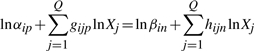(3)

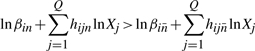
which can be written in matrix form as simply

(4)

where y_j = lnX_j, a_ij = g_ijp − h_ijn and b_i = ln(β_in/α_ip). Note that A is an M × Q matrix whose elements represent the differences in the dominant kinetic orders, g_ijp and h_ijn. Furthermore, the dependent and independent concentration variables can be split, such that

(5)

where A_D is an M × M square matrix. It follows that the steady states of the dependent concentrations, in logarithmic terms, are

(6)

The result shows that by assuming a dominant positive and negative term in each equation, we can calculate an approximate steady state using linear algebra.

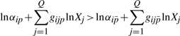
The assumption that some terms dominate implies certain conditions, which are represented by inequalities of the form

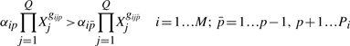(7)

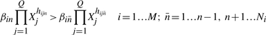(8)

Again, p and n are the indices of the dominant positive and negative terms in the i-th equation, while and are the sets of indices of non-dominant terms. Taking the logarithm of both sides yields

(9)

(10)

All the conditions can be listed in matrix form as

(11)

with y_j = lnX_j, , , and 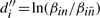, or simply

(12)

C is an R × Q matrix, where R is the total number of conditions. As in the steady state analysis, the dependent and independent variables can be split, such that

(13)

The steady state solution, Equation (6), can be combined with Equation (13) to form

(14)

where U = C_I − C_DA_D⁻¹A_I and W = C_DA_D⁻¹. Equation (14) is solely a function of the independent parameters: independent concentrations, rate constants and kinetic orders. As such, it serves as a standard definition of the boundary conditions in design space. Clearly, the boundaries themselves are described by

(15)

The terms boundary conditions and boundaries are used interchangeably when the meaning is made clear by the context. In design space, the boundaries enclose a region of parameter values for which the designated terms dominate and describe a dominant behavior. The approximation is best when far from the boundaries and worsens near them. Nevertheless, the boundaries indicate a transition from one approximation to another, effectively separating qualitatively distinct phenotypes of the system.

2.2 Rate constants

Rate constants can be related. For example, stoichiometry implies a linear relationship, such as α₂₁ = 2β₁₁. To capture such relationships, and without loss of generality, we can treat each rate constant as a function of independent parameters, X_j, with associated kinetic orders. Consequently, all α_ik and β_ik in our algorithms represent constant coefficients, and arrays that are based on them, such as b and d, are numeric. All independent concentrations and rate constants are contained in y_I.

2.3 Kinetic orders

In Equation (15), the elements of matrices U and W are rational functions of the kinetic orders. If the kinetic orders are assigned constant values, then the equation clearly shows that the boundaries are linear in the logarithm of the rate constants and independent concentrations. All work that has utilized the generic construction of design space has dealt with constant kinetic orders and, therefore, linear boundaries in design space (Coelho et al., 2009; Savageau and Fasani, 2009; Savageau et al., 2009).

However, we may wish to vary one or more kinetic orders and search for an underlying design principle. In fact, past handcrafted design spaces have illustrated the impact of varying a kinetic order (Atkinson et al., 2003; Hlavacek and Savageau, 1995, 1996; Savageau, 1974, 2001, 2002). In the case of variable kinetic orders, Equation (15) forms boundaries that are typically nonlinear in logarithmic coordinates.

As might be expected, linear boundaries allow for a broader class of tools, especially from the field of linear programming, to help automate the analysis of design space. The following algorithms assume that the kinetic orders of the system are constant, unless otherwise noted. We consider methods for dealing with variable kinetic orders in the final discussion.

3 CONSTRUCTION OF DESIGN SPACE

3.1 Enumerating cases

The first step of design space construction is the enumeration of all possible dominant S-systems and their conditions for dominance. The task requires organizing, indexing and manipulating the terms of the original GMA model. We begin by counting the positive and negative terms in each equation and, by convention, listing the results in the form

(16)

which we call the system signature. Every positive and negative term is potentially dominant, and each combination of dominant terms is referred to as a case. The total number of cases, T, is a straightforward product of the entries in the system signature, or

(17)

For a particular case, the indices of the dominant terms are listed in the same order, as

(18)

A list of dominant indices is called a case signature, and uniquely identifies a case. However, for the sake of brevity, cases are also numbered. By convention, case numbers are assigned sequentially, as if counting, where the list of dominant indices is considered a number with the least significant digit on the right. Case 1, then, is when the first positive and first negative term in every equation is dominant, or [1, 1, … 1, 1]; case 2 is the same, except that the second negative term in the last equation, if it exists, is dominant, or [1, 1, … 1, 2]; and so on. For example, consider the simple GMA model

(19)

(20)

Each equation has one positive term and two negative terms, making the system signature [1, 2, 1, 2]. The four cases are as follows:

Case 1: [1, 1, 1, 1]

Case 2: [1, 1, 1, 2]

Case 3: [1, 2, 1, 1]

Case 4: [1, 2, 1, 2]

In case 1, the first negative term dominates in both equations. Case 2 is the same, except the second negative term in the second equation dominates. There is only one positive term in the second equation, so case 3 is the same as case 1, except the second negative term in the first equation dominates. In fact, the first and third indices never change because there is only one positive term in each equation; nevertheless, the indices are kept in place for consistency and clarity.

In each case, the dominant terms are linked to conditions, which are enumerated as described in Section 2.1. The number of conditions, R, can be determined by

(21)

and is the same for every case. Therefore, the total number of conditions is simply the product RT. Clearly, the number of conditions grows quickly as the number of terms, P_i or N_i, increases, and is therefore likely to have the largest impact on the scalability of the methods. However, every condition has an opposite. In one case, a first term may dominate over a second; in another case, the second will dominate over the first. Hence, among all the enumerated conditions, each inequality of the form a > 0 will have an opposite of the form a < 0 or −a > 0, which halves the number of equations that must be stored. Similarly, the total number of boundary conditions is RT, while the number of boundaries is RT/2.

Furthermore, many of the conditions are duplicates: a condition that appears in one case will also appear in another. Each equation represents a set of possible conditions, and each case is a different combination of those conditions. It can be shown that the number of unique conditions for a system is

(22)

which is smaller than RT. Again, each unique condition has an opposite, halving the number of equations that must be stored. Clearly, scalability is a concern, one we return to in the final discussion.

3.2 Validating cases

Next, each case should be checked for validity. Typically, boundaries enclose a region in design space. In some cases, the boundaries are mutually exclusive, implying that a corresponding region does not exist. Cases that do not enclose a region are called invalid. If the matrix A_{_D} in Equation (5) is singular, the problem can be resolved by reformulating the original equations.

Consider the standard form of the boundary conditions in Equation (14). In the case of constant kinetic orders, the boundaries are linear and may enclose an n-dimensional convex polytope. Specifically, the boundaries take the simplified form

(23)

where z = Wb+d represents a column vector of numeric values.

The linear inequalities of Equation (23) are similar to the constraints used in linear programming (Dantzig, 1963; Vanderbei, 2008). In fact, one task in linear programming, sometimes called Phase I, is to verify the existence of a feasible region, or a region that satisfies the constraints. It follows that if we can reformulate the boundaries in terms of a standard linear programming problem, we can use existing linear programming algorithms to determine if the case is feasible or valid. To do so, we add a slack variable to convert the strict inequalities to standard inequalities. The resulting linear programming problem is

(24)

If the slack variable ε can be minimized to a negative number, then a feasible region exists and the case is valid. Furthermore, the algorithm will terminate at an optimal point, y_I0, which represents one point in the valid region and helps locate the region within the multidimensional design space.

3.3 Plotting and visualization

The most direct method of depicting design space is based on sampling: we evaluate the boundary conditions in Equation (14) at a given point, or a specific combination of parameter values. If all the boundary conditions for a case are satisfied, then the point lies within the associated region. A point can satisfy multiple cases or lie within multiple regions. Consequently, every point must be tested over every valid case. By setting all but a few parameters to specific values, and uniformly sampling the remaining two or three parameters, we can draw a 2-dimensional or 3-dimensional slice of design space. We can increase the resolution by increasing the number of sampled points. The method can be applied to systems with constant or variable kinetic orders, and although it is computationally intensive, it is highly parallelizable.

4 ANALYSIS OF DESIGN SPACE

4.1 Searching for intersections

Regions in design space can intersect. The subregion of intersection contains parameter combinations for which the system can exhibit multiple steady states. Instances of three intersecting regions are particularly interesting as they indicate the potential for bistable hysteretic behavior (Savageau and Fasani, 2009). Finding intersecting regions on a finite 2-dimensional plot is a straightforward visual task. Exhaustively searching a higher dimensional design space for intersecting regions requires a different approach.

To determine whether a group of regions intersect, we extend the process of validation. We combine the boundaries of every region in question, and test if the combined set of boundaries is valid; if valid, the regions intersect and the combined boundaries enclose a subregion of intersection. To search all of design space for intersections, we test every possible combination of regions. Hence, to search for instances of three intersecting regions, we check T!/(3!(T − 3)!) combinations, where T is the total number of cases, as shown in Equation (17). To exhaustively search for every intersection, we repeat the process for instances of 2 through T intersecting regions, which, in the worst case, requires

(25)

tests. However, only valid regions, or cases, need be tested. Furthermore, if the numbers 2 through T are checked in order, only subregions that are the result of i intersecting regions and share all but two intersecting regions need be tested for (i + 1) intersecting regions. For example, subregions {1, 2, 3} and {1, 2, 4} should be checked for the intersection of {1, 2, 3, 4}. In practice, the number of tests is much smaller than Equation (25) suggests.

4.2 Bounding a region

Once we identify a valid region or subregion of intersection, we would like to locate it within design space and determine its extent. We can do so, at least approximately, by automatically forming an axis aligned bounding box around the region of interest. In the case of constant kinetic orders, the region is a convex polytope in design space, and we can construct a bounding box around the region via linear programming. If the number of independent parameters is defined by L = Q − M, then the bounding box can be found via 2L linear programming problems of the forms

(26)

and

(27)

Optionally, the bounds of each y_Ij can be described by additional constraints and updated after each step. Although 2L linear programming problems seems computationally expensive, algorithms that employ a primal-dual simplex method with hot starts appear to significantly reduce the number of operations (Yamamura and Fujioka, 2003; Yamamura et al., 2009). Furthermore, each linear programming problem may return an optimal point, y_I0, which represents a vertex of the valid region and helps locate the region in the multidimensional design space.

4.3 Measuring tolerance

Tolerance is defined as the fold change in one parameter required to move from an operating point in one region to an adjacent region of design space (Coelho et al., 2009). In other words, it is the distance from a point in design space to the nearest boundary while moving along a straight line parallel to a parameter axis. If we vary only one parameter, then the boundaries, described by Equation (15), become a set of univariate functions, and determining where the line intersects the boundaries is a univariate root-finding problem.

In the case of constant kinetic orders, only one element of y_I varies, making Equation (15) a set of linear equations. We can easily solve each equation, and the root closest the operating point, on either side, determines the tolerance. Specifically, the tolerance is the absolute distance from the operating point to the root, in logarithmic coordinates, and is equivalent to a fold change in Cartesian coordinates. If a root does not exist on one side of the operating point, the tolerance to change in that direction is infinite.

In the case of variable kinetic orders, the elements of U and W are rational functions of the varying parameter. Consequently, Equation (15) becomes a set of rational functions in one variable, and measuring tolerance is equivalent to finding the roots of univariate polynomials, for which several modern approaches and tools can be used (Mehlhorn and Sagraloff, 2009; Mourrain and Pavone, 2009; Pan, 1997, 2001). Again, the distance from the operating point to the closest roots determines the tolerance to change for a given parameter.

4.4 Local analysis

In each case, the dominant S-system can be analyzed via established methods. For small changes in the variables and parameters, the signal amplification of the system can be quantified via logarithmic gain, defined as L(X_i, X_j) = ∂lnX_i/∂lnX_j (Savageau, 1971a). Likewise, robustness is associated with parameter sensitivity, defined as S(X_i, p_j) = ∂lnX_i/∂lnp_j (Savageau, 1971b). The eigenvalues of the linearized system indicate local stability and response time (Savageau, 1975).

Traditionally, parameter sensitivity measures the change with respect to a single rate constant or kinetic order, as in S(X_i, α_j ) or S(X_i, g_jk). Here, we consider the case where multiple rate constants or kinetic orders are a function of some changing parameter p_j. By treating variable rate constants as independent variables, as described in Section 2.2, we already account for a parameter that appears as a rate constant, or coefficient, in several terms. For variable kinetic orders, the traditional measure of sensitivity must be extended. It can be shown that

(28)

where X_D is the vector of all dependent concentrations at steady state. As defined in Section 2.1, y is a vector that represents the logarithm of all concentrations, and the elements of matrices A and A_D are differences in the kinetic orders. The sensitivity of the flux to a change in p is

(29)

where G is the matrix of kinetic orders from the dominant terms, or all g_ijp in Equation (3), and V_D is the vector of steady fluxes through the pools represented by X_D, defined by ln V_D = lnα + GlnX_D. If p_j represents just a single kinetic order, or p_j = g_jk, then Equation (28) reduces to the traditional measure of steady state sensitivity with respect to a kinetic order: S(X_i, g_jk) = (A_D⁻¹)_ijg_jky_k. Similarly, Equation (29) reduces to the traditional measure of steady flux sensitivity with respect to a kinetic order.

By calculating logarithmic gains, parameter sensitivities and eigenvalues for the dominant S-system in each case, or region, we can characterize the distinct phenotypes of the system. Given a set of performance criteria, the fitness of each phenotype can be quantitatively compared.

5 IMPLEMENTATION

The described algorithms have been implemented and packaged as the Design Space Toolbox for MATLAB®, a numerical programming environment with the necessary tools for matrix manipulation, symbolic manipulation, linear programming, root finding and plotting. The Design Space Toolbox requires the object oriented facilities introduced in MATLAB 7.6 (R2008a). All tests were performed on a MacBook Pro with 2.93 GHz Intel Core 2 Duo, running OS X 10.5.8 and MATLAB 7.8 (R2009a). The distributed package includes installation instructions, extensive documentation and several demonstrations that introduce design space concepts and procedures. The source code has been released under the BSD license, and the toolbox is freely available at http://www.bme.ucdavis.edu/savageaulab/.

6 RESULTS

6.1 An example system

Consider the abstract model

(30)

(31)

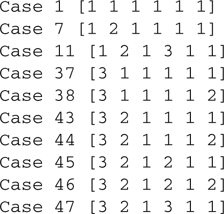
Assume all variables are normalized and therefore dimensionless. The dependent concentrations are X₁ and X₂. The three varying parameters are the rate constant, α, and the two independent concentrations, X₃ and X₄, implying that the full design space is 3-dimensional. There are two positive and two negative terms in each equation, yielding 16 cases. We used the Design Space Toolbox to automatically enumerate the cases and test each one for validity. The toolbox listed the valid cases as

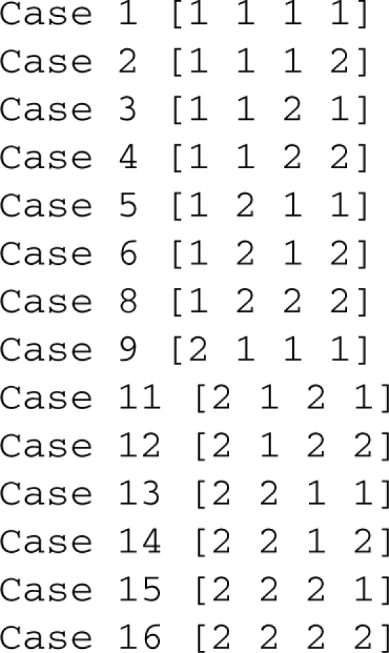
Careful inspection of the output reveals that cases 7 and 10 are invalid. We can manually confirm the results by examining the boundary conditions. For case 7, the boundary conditions are as follows:

(32)

(33)

(34)

(35)

Simple inspection reveals that Equations (32) and (33) are mutually exclusive, as well as Equations (34) and (35), confirming that the case is invalid. Likewise, the boundary conditions for case 10 are as follows:

(36)

(37)

(38)

(39)

Again, inspection confirms that the conditions are mutually exclusive and the case is invalid.

We arbitrarily assumed α = 10 and used the Design Space Toolbox to draw the resulting 2-dimensional design space, a function of X₃ and X₄, in Figure 1a. Only some of the valid regions are evident. Recall that the full design space of the system is 3-dimensional, meaning Figure 1a is but one slice of the whole. We explored the design space by changing α, and chose a second slice, evaluated at α = 0.1, for Figure 1b. Together, the two slices display every valid region. Figure 1c shows a slice perpendicular to the first two, revealing how some of the regions vary with α.

Fig. 1.

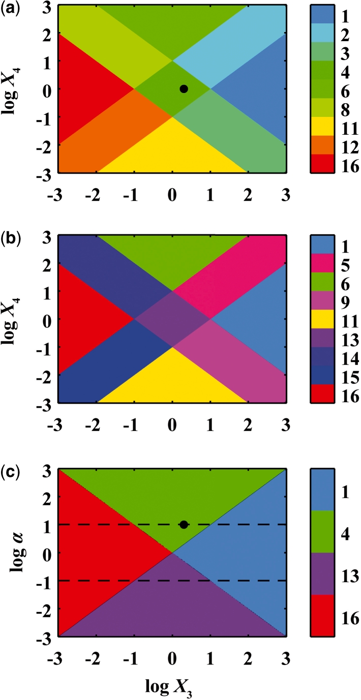
Visualization of the design space for the example system when varying parameters X₃, X₄ and α, colored by region number; (a) slice at α = 10; (b) slice at α = 0.1; (c) slice at X₄ = 1; dashed line, location of a slice; filled circle, normal operating point.

Assuming the normal operating point is at α = 10, X₃ = 2 and X₄ = 1, Figure 1a shows that the system normally exhibits the phenotype associated with region 4. We used the Design Space Toolbox to measure the tolerance, or the parameter change required to move into an adjacent region. The output, where the tolerance to a fold change down and a fold change up is denoted [T_low, T_high], was

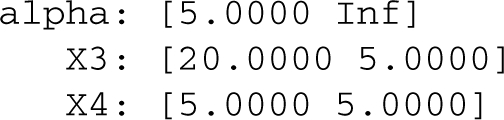
X₄ can tolerate a 5-fold increase or decrease before moving out of region 4, which can be seen as a 0.7 shift up or down on the logarithmic scale of Figure 1a. Similarly, α can tolerate a 5-fold decrease, but is effectively unbounded upward, as shown in Figure 1c. X₃ can tolerate a 5-fold increase and a 20-fold decrease, which is evident in both Figures 1a and c.

Although tolerance indicates the system will cross a boundary at α = 2 when starting from the operating point and changing a single parameter, other combinations of parameters in the region may allow a smaller α. We used the Design Space Toolbox to find the overall parameter bounds for region 4. The output, expressed as an interval over the positive real numbers, was

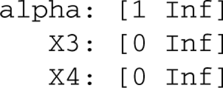
The minimum value of α in the region is 1. Also, X₃ and X₄ can take on any positive value, meaning they are unbounded in logarithmic coordinates, as Figure 1c suggests.

With the example, we have demonstrated how the Design Space Toolbox can be used to automatically construct, analyze and explore a relatively small design space. The tools are even more useful during practical application, when the models and design spaces grow larger.

6.2 Lambda phage lysogeny

A design space for the gene circuit controlling lambda phage lysogeny was recently constructed and analyzed (Savageau and Fasani, 2009). Of particular interest were the bistable regions of hysteresis. The GMA model at steady state was normalized and recast to

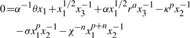(40)

(41)

(42)

x₁ represents the concentration of the repressor CI dimer, normalized to its low concentration at the fully induced, lytic state. The dimer activates its own transcription at low concentrations and represses transcription at high concentrations; the normalized threshold of half-maximal activation is κ. r represents the external signal, RecA*, that stimulates CI degradation, normalized to its concentration at half-maximal activation. The other normalized, dimensionless parameters were estimated based on experimental data: χ = 320, ϕ = 10, α = 215, σ = 7.1, θ = 2, a = 1, p = 3 and n = 1.5. κ was constrained to the range [1, 10 000] and r was constrained to the range [0.001, 10].

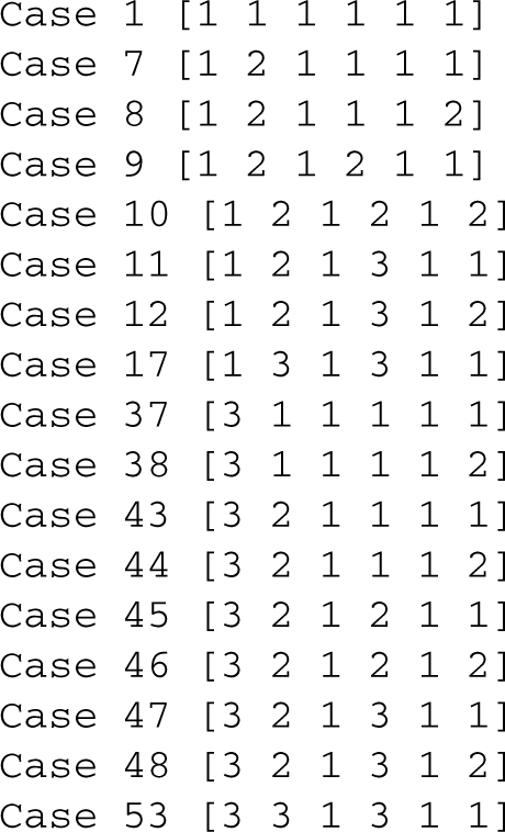
We used the Design Space Toolbox to reconstruct the design space and check for valid cases within the constrained region. The output

verifies the original results. Furthermore, we used the Design Space Toolbox to visualize the design space over the same range of parameters. The output, shown in Figure 2a, again verifies the original results. As the external signal r varies within a range of κ, the system switches between lysogenic and lytic growth across a hysteretic buffer. Local analysis emphasizes the fact: we used the Design Space Toolbox to calculate the steady state of the CI repressor for a slowly increasing signal, shown in Figure 2b, and for a slowly decreasing signal, shown in Figure 2c. As the external signal r increases from its low value in lysogeny, the CI repressor concentration remains high through a buffer zone and then abruptly decreases, triggering induction. If the direction is reversed, the system must pass back through the buffer before the repressor concentration increases, an all-or-nothing response that is a hallmark of hysteretic behavior. Furthermore, the figures indicate that the switching only occurs over a certain range of parameter values.

Fig. 2.

Visualization of the design space for lambda phage lysogeny control when varying the signal concentration, r, and the CI dimer concentration needed for half-maximal activation of transcription, κ. Filled circle, normal lysogenic operating point; open circle, normal lytic operating point; dashed line, upper and lower bounds of effective switching between lysogenic and lytic growth; (a) regions colored by region number; (b) steady state of the CI dimer, x₁, for slowly increasing signal; (c) steady state of the CI dimer, x₁, for slowly decreasing signal.

As was seen in Figure 1a, the 2-dimensional slice of design space in Figure 2a may not contain all of the valid regions. We varied five of the parameters, χ, ϕ, α, σ and θ, 2-fold above and below their original values and used the Design Space Toolbox to check for valid regions within the resulting 7-dimensional design space. The output

indicates that there are seven other valid regions relatively near the normal operating point. Furthermore, we used the Design Space Toolbox to find every subregion of intersection, or potential region of hysteresis, in the same range. The output

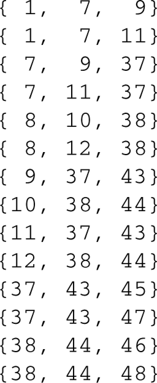
not only verifies the original subregions of intersection, shown in Figure 2a, but also indicates that there are eight other regions of potential hysteresis relatively close to the original analysis.

Extending the search, we used the Design Space Toolbox to check for valid regions over the unbounded range of all seven parameters. Clearly, physical parameters are limited in the extremes—rate constants cannot exceed the diffusion limit and independent concentrations cannot exceed the solubility limit, for example—but an analysis over the infinite range provides an upper bound on the number of valid regions and intersections. We found that 42 of the 54 regions are valid somewhere in the design space. Furthermore, we found 73 regions of potential hysteresis. Remarkably, every one of the 42 valid regions intersects a region of potential hysteresis. Some of the newly discovered regions may not be biologically relevant, but the rest may be worthy of further analysis. As such, we have shown that the Design Space Toolbox can automate existing analyses, as well as perform more difficult analyses that would be prohibitive if done manually.

7 DISCUSSION AND CONCLUSION

Design space has proven a useful tool in the analysis of biochemical systems. Within design space, we can enumerate the phenotypic repertoire of a system model over a wide range—even an infinite range—of parameter values. However, for all but the smallest models, constructing and analyzing the design space is manually infeasible. Here, we have shown that the process can be automated.

In the case of constant kinetic orders, the boundaries of design space are linear, and linear programming can be employed in the automated analysis of the regions. Unfortunately, in the case of variable kinetic orders, the boundaries are usually nonlinear, obviating the use of linear programming. Nevertheless, we could inspect the boundaries for special forms (e.g. linear, quadratic or convex) and, under favorable conditions, use an appropriate variety of convex programming (Boyd and Vandenberghe, 2004) to determine validity and bound the region. Alternatively, we could employ subdivision strategies to build a piecewise-linear approximation of the region and handle each subpolytope separately.

How closely the bounding box encloses the region of interest depends on the shape and orientation of the polytope. For a better, yet more computationally expensive, description of the region, we could employ vertex or face enumeration techniques (Avis and Fukuda, 1992; Avis et al., 1997). Such a method would require more computation and storage, and be harder to conceptualize, but would give an exact description of the convex polytope that represents a region in design space.

When measuring tolerance, we might want to measure the distance to some arbitrary boundary, rather than the boundaries of the region. For example, in Figure 1a, we could measure tolerance from the typical lysogenic operating point to the dashed lines that represent the boundaries of effective switching between lysogenic and lytic growth, which are not actually boundaries of the enclosing region. Alternatively, we could join several regions of similar phenotypes and measure tolerance to the boundary of the composite region, effectively measuring tolerance across several regions. Either case suggests that we would like to add, extend or in other ways manipulate the boundaries of design space according to additional knowledge, especially regarding the biology of the system.

At various points, we have mentioned the challenge of scalability, or handling larger systems and design spaces. The size of the problem is not just dependent on the number of variables and equations but also on the number of parameters and terms—more terms produce significantly more cases. We have successfully applied the Design Space Toolbox to moderately sized systems with tens of parameters and thousands of cases. To handle millions of cases, we can take advantage of the parallel nature of the algorithms and analyze each case independently. We plan to update the Design Space Toolbox to utilize multiple processors, enabling it to handle more cases in practical time. As for thousands of parameters, any case with constant kinetic orders is analyzed with linear algebra and linear programming, for which existing computational libraries are known to scale well.

With that said, we have presented a detailed description of design space construction and analysis, and have described algorithms to automate the common tasks. Furthermore, we have noted the conditions under which the various algorithms can be used effectively. Specifically, we have extended the concepts to include models with variable kinetic orders, and have discussed the challenges such models present. We have also discussed the issue of scaling to larger systems and design spaces. In the end, we have created a working implementation of the algorithms: the Design Space Toolbox for MATLAB. We have demonstrated it using both abstract and biological examples, and made it freely available for others to explore the design space of biochemical systems.

REFERENCES

- Atkinson MR, et al. Development of genetic circuitry exhibiting toggle switch or oscillatory behavior in Escherichia coli. Cell. 2003;113:597–607. doi: 10.1016/s0092-8674(03)00346-5. [DOI] [PubMed] [Google Scholar]
- Avis D, Fukuda K. A pivoting algorithm for convex hulls and vertex enumeration of arrangements and polyhedra. Discrete Comput. Geom. 1992;8:295–313. [Google Scholar]
- Avis D, et al. How good are convex hull algorithms? Comput. Geom. 1997;7:265–301. [Google Scholar]
- Boyd SP, Vandenberghe L. Convex Optimization. Cambridge, UK: Cambridge University Press; 2004. [Google Scholar]
- Coelho PM, et al. Quantifying global tolerance of biochemical systems: design implications for moiety-transfer cycles. PLoS Comput. Biol. 2009;5:e1000319. doi: 10.1371/journal.pcbi.1000319. [DOI] [PMC free article] [PubMed] [Google Scholar]
- Dantzig GB. Linear Programming and Extensions. Princeton, NJ: Princeton University Press; 1963. [Google Scholar]
- Hlavacek WS, Savageau MA. Subunit structure of regulator proteins influences the design of gene circuitry: analysis of perfectly coupled and completely uncoupled circuits. J. Mol. Biol. 1995;248:739–755. doi: 10.1006/jmbi.1995.0257. [DOI] [PubMed] [Google Scholar]
- Hlavacek WS, Savageau MA. Rules for coupled expression of regulator and effector genes in inducible circuits. J. Mol. Biol. 1996;255:121–139. doi: 10.1006/jmbi.1996.0011. [DOI] [PubMed] [Google Scholar]
- Lander ES, et al. Initial sequencing and analysis of the human genome. Nature. 2001;409:860–921. doi: 10.1038/35057062. [DOI] [PubMed] [Google Scholar]
- Mehlhorn K, Sagraloff M. Proceedings of the 2009 International Symposium on Symbolic and Algebraic Computation. Seoul, Republic of Korea: ACM; 2009. Isolating real roots of real polynomials; pp. 247–254. [Google Scholar]
- Metzker ML. Sequencing technologies - the next generation. Nat. Rev. Genet. 2010;11:31–46. doi: 10.1038/nrg2626. [DOI] [PubMed] [Google Scholar]
- Mourrain B, Pavone JP. Subdivision methods for solving polynomial equations. J. Symbolic Comput. 2009;44:292–306. [Google Scholar]
- Pan VY. Solving a polynomial equation: some history and recent progress. SIAM Rev. 1997;39:187–220. [Google Scholar]
- Pan VY. Proceedings of the 2001 International Symposium on Symbolic and Algebraic Computation. London, Ontario, Canada: ACM; 2001. Univariate polynomials: nearly optimal algorithms for factorization and rootfinding; pp. 253–267. [Google Scholar]
- Sanger F, et al. DNA sequencing with chain-terminating inhibitors. Proc. Natl Acad. Sci. USA. 1977;74:5463–5467. doi: 10.1073/pnas.74.12.5463. [DOI] [PMC free article] [PubMed] [Google Scholar]
- Savageau MA. Concepts relating the behavior of biochemical systems to their underlying molecular properties. Arch. Biochem. Biophys. 1971a;145:612–621. doi: 10.1016/s0003-9861(71)80021-8. [DOI] [PubMed] [Google Scholar]
- Savageau MA. Parameter sensitivity as a criterion for evaluating and comparing the performance of biochemical systems. Nature. 1971b;229:542–544. doi: 10.1038/229542a0. [DOI] [PubMed] [Google Scholar]
- Savageau MA. Comparison of classical and autogenous systems of regulation in inducible operons. Nature. 1974;252:546–549. doi: 10.1038/252546a0. [DOI] [PubMed] [Google Scholar]
- Savageau MA. Optimal design of feedback control by inhibition. J. Mol. Evol. 1975;5:199–222. doi: 10.1007/BF01741242. [DOI] [PubMed] [Google Scholar]
- Savageau MA. Design principles for elementary gene circuits: elements, methods, and examples. Chaos. 2001;11:142–159. doi: 10.1063/1.1349892. [DOI] [PubMed] [Google Scholar]
- Savageau MA. Alternative designs for a genetic switch: analysis of switching times using the piecewise power-law representation. Math. Biosci. 2002;180:237–253. doi: 10.1016/s0025-5564(02)00113-x. [DOI] [PubMed] [Google Scholar]
- Savageau MA. Biochemical Systems Analysis: A Study of Function and Design in Molecular Biology. Reading, MA: Reprint of the original edition published by Addison-Wesley; 2009. 1976. [Google Scholar]
- Savageau MA, Fasani RA. Qualitatively distinct phenotypes in the design space of biochemical systems. FEBS Lett. 2009;583:3914–3922. doi: 10.1016/j.febslet.2009.10.073. [DOI] [PMC free article] [PubMed] [Google Scholar]
- Savageau MA, Voit EO. Recasting nonlinear differential equations as S-systems: a canonical nonlinear form. Math. Biosci. 1987;87:83–115. [Google Scholar]
- Savageau MA, et al. Phenotypes and tolerances in the design space of biochemical systems. Proc. Natl Acad. Sci. USA. 2009;106:6435–6440. doi: 10.1073/pnas.0809869106. [DOI] [PMC free article] [PubMed] [Google Scholar]
- Shendure J, Ji H. Next-generation DNA sequencing. Nat. Biotechnol. 2008;26:1135–1145. doi: 10.1038/nbt1486. [DOI] [PubMed] [Google Scholar]
- Vanderbei RJ. Linear Programming: Foundations and Extensions. New York: Springer; 2008. [Google Scholar]
- Venter JC, et al. The sequence of the human genome. Science. 2001;291:1304–1351. doi: 10.1126/science.1058040. [DOI] [PubMed] [Google Scholar]
- Yamamura K, Fujioka T. Finding all solutions of nonlinear equations using the dual simplex method. J. Comput. Appl. Math. 2003;152:587–595. [Google Scholar]
- Yamamura K, et al. LP narrowing: a new strategy for finding all solutions of nonlinear equations. Appl. Math. Comput. 2009;215:405–413. [Google Scholar]