Logic Forest: an ensemble classifier for discovering logical combinations of binary markers

Abstract

Motivation: Highly sensitive and specific screening tools may reduce disease -related mortality by enabling physicians to diagnose diseases in asymptomatic patients or at-risk individuals. Diagnostic tests based on multiple biomarkers may achieve the needed sensitivity and specificity to realize this clinical gain.

Results: Logic regression, a multivariable regression method predicting an outcome using logical combinations of binary predictors, yields interpretable models of the complex interactions in biologic systems. However, its performance degrades in noisy data. We extend logic regression for classification to an ensemble of logic trees (Logic Forest, LF). We conduct simulation studies comparing the ability of logic regression and LF to identify variable interactions predictive of disease status. Our findings indicate LF is superior to logic regression for identifying important predictors. We apply our method to single nucleotide polymorphism data to determine associations of genetic and health factors with periodontal disease.

Availability: LF code is publicly available on CRAN, http://cran.r-project.org/.

Contact: wolfb@musc.edu

Supplementary information: Supplementary data are available at Bioinformatics online.

1 INTRODUCTION

Diseases often stem from complex gene–gene and gene–environment interactions and single biomarkers typically perform poorly with respect to sensitivity and specificity (Alvarez-Castro and Carlborg, 2007; Kotti et al., 2007; Kumar et al., 2006). Lo and Zhang (2002) note that common statistical methods for screening high-dimensional biomarker data focus on only main effects and do not capture interactions that lead to disease. Failure to recognize interactions among genes leads to the inability to replicate study results in human populations (Carlborg and Haley, 2004). Many authors suggest that a panel of biomarkers rather than a single marker has the potential to provide improvements in sensitivity and specificity required to replace traditional diagnosis (see, e.g. Kumar et al., 2006; Manne et al., 2005; Srivastava, 2005). Diseases for which panels of markers demonstrate improved sensitivity and specificity over single markers include prostate, ovarian and bladder cancer and heart disease (Manne et al., 2005; Negm et al., 2002; Wagner et al., 2004; Zethelius et al., 2008).

Non-parametric tree-based methods are easily interpretable and have flexibility to identify relationships among predictor variables (Austin, 2007). Logic regression (LR; Ruczinski et al., 2003) is a tree-based method capable of modeling a binary, continuous or survival response with higher order interactions among binary predictors. In this article, we focus on classification of a binary response. LR generates classification rules by constructing Boolean (‘and’ = ∧, ‘or’ = ν , and ‘not’ = !) combinations of binary predictors for classification of a binary outcome. An LR model is represented as a tree with connecting nodes as the logical operators and terminal nodes (called leaves) as the predictors. LR has been used in the development of screening and diagnostic tools for several diseases and has shown modest improvements in sensitivity and specificity compared with traditional approaches such as logistic regression and CART (Etzioni et al., 2003, 2004; Janes et al., 2005; Kooperberg et al., 2007; Vermeulen et al., 2007).

LR can be unstable when data are noisy. In the context of identifying interacting genetic loci, performance was poor for frequently occurring interactions only weakly associated with the response (Vermeulen et al., 2007). A study designed to identify regulatory motifs confirmed that increasing noise in data severely limited the ability of LR to correctly identify the true model in simulated data (Keles et al., 2004). Ensemble extensions of tree-based methods demonstrate improved predictive accuracy (Breiman, 1996; Dietterich, 2000; Friedman, 2001). Two ensemble adaptations of LR are available. Monte Carlo LR (MCLR) builds a series of models from the training dataset using Monte Carlo methods and identifies groups of predictors that co-occur across all models (Kooperberg and Ruczinski, 2005). However, the relationship among predictors (∧, ν and !) is unclear. LogicFS, a bagging version of LR, constructs an ensemble by drawing repeated bootstrap samples and building LR models from each (Breiman, 1996; Schwender and Ickstadt, 2008). In contrast to MCLR, logicFS identifies explicit predictor interactions [referred to as prime implicants (PIs)]. Additionally, logicFS provides a measure of variable interaction importance.

In Section 2, we present a new ensemble of logic trees approach called Logic Forest (LF), and introduce a new permutation-based measure of predictor importance. We also develop the idea of subset matching as an additional means of identifying important interactions. We present a simulation study in Section 3 comparing the performance of LR and logicFS with LF considering data with noise in the predictors, latent predictors and varying true model complexity. We apply LF to periodontal disease data in Section 4 and discuss the results of our simulation studies in Section 5.

2 DEFINITIONS AND NOTATION

2.1 LF

Given observed data W = (y, x) recorded on n subjects consisting of a binary response y = (y₁,…, y_n)^′ and p binary predictors x_i = (x_i1,…, x_ip), i = 1,…, n, LR constructs a tree T describing Boolean combinations of predictors that best classify the response. For example, LR might produce the expression T = (X₄ ν X₁₁) ∧ X₅. A logic expression (i.e. tree) can be expressed in reduced disjunctive normal form (DNF), defined as a series of PIs joined by ν operators (Fleisher et al., 1983). PIs capture predictor interactions as ∧ combinations that cannot be further reduced (Schwender and Ickstadt, 2008). For example T₂ = (X₃ ∧ X₄ ∧ X₅) ν (X₃ ∧ X₅ ∧ X₁₁) ν (X₃ ∧ !X₃ ∧ X₅) is the DNF of the expression T₁ = (X₄ ν X₁₁ ν !X₃) ∧ (X₅ ∧ X₃). T₂, however, is not in reduced DNF as its third term can be further simplified yielding the three PI reduced DNF form, T₃ = (X₃ ∧ X₄ ∧ X₅) ν (X₃ ∧ X₅ ∧ X₁₁) ν X₅. Henceforth, all logic expressions will be in reduced DNF. The complexity of a tree is defined by the size and number of PIs. A PI's size is defined as the number of predictors in the PI. Given an LR model, LR(W) = T, and a new observation consisting of predictors x with dimension 1 × p, the prediction made by T is taking values 0 or 1.

The LF of B trees, denoted LF(W, B) = {T¹,…, T^B} = {T^b}, b=1,…, B, is an ensemble of LR trees constructed from B bootstrap samples, W^b, from W. For each b, a positive integer M^b is selected limiting the size of tree T^b in the ensemble by specifying the maximum number of terminal nodes (leaves); thus, random selection of M^b from within specified ranges ensures variability of tree sizes within LF.

Given values for the p predictors for m new observations, x* (an m × p matrix), and a forest of B trees LF(W, B), the predicted values, , are based on a majority vote so that

(1)

where x_ℓ^* is the ℓ^th row of x*. Given response y* = {y₁^*,…, y_m^*} for x*, we calculate the misclassification rate as:

(2)

Associated with tree b in the forest is an out-of-bag dataset, OOB (T^b), comprising observations not included in the bootstrap sample used to construct T^b. If test data are not available, we can use OOB (T^b) to obtain an unbiased estimate of the forest's misclassification rate. Let W_i = (y_i, x_i) ∈ W, and let O (W_i, T^b) = I (W_i ∈ OOB (T^b)) indicate the i-th observation's membership in OOB (T^b). The LF OOB prediction is

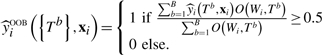(3)

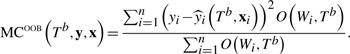
The LF OOB misclassification rate is

(4)

2.2 Variable importance measures

Let X be a predictor or, more generally, a PI occurring in the tree. The importance of X in an LR model, VIMP.LR(X), is determined by X's presence or absence in a fitted tree, T, providing a crude assessment of association with response.

An advantage of LF over LR is the availability of many trees for identifying important predictors and PIs. Our LF importance measure for predictor X_j, j = 1,…, p, is based on the misclassification rates for each tree in the forest. Denote the OOB misclassification rate for T^b by

(5)

Let x^(j) denote the matrix of predictors with X_j randomly permuted. We define the variable importance measure for X_j by

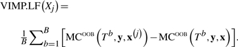(6)

Values range between −1 and 1, with positive values suggesting a positive association between response, Y, and predictor X_j. More generally, (6) can be computed with X_j being a PI.

An algorithm similar to LF, called logicFS, was introduced by Schwender and Ickstadt (2008). Unlike logicFS, LF randomly selects the maximum size when building each tree in the ensemble. Although tree size can vary in logicFS, flexibility in the upper bound for the maximum number of leaves in a tree enhances the probability that the forest will discover smaller PIs. Additionally, Schwender and Ickstadt provide a different measure of PI importance obtained by replacing the permutation step in (6) with addition or removal of the PI in tree T^b, which we will refer to as VIMP.FS (Schwender and Ickstadt, 2008).

2.3 Subset matching

Let F be the set of unique PIs identified in a LF consisting of B trees. When a given PI, P for example, is an element of F, we say P is an ‘exact match’. We say P is a ‘subset match’ for a forest if P is an exact match or P ∧ Q is an element of F for some PI, Q. For example, LF might identify PI₁=X₄∧X₅ and PI₂=X₄∧X₅∧X₆. The PI X₄∧X₅ is an exact match to PI₁ and a subset match to PI₂. The concept of subset matching enables us to fully detect contributions of PIs to the fitted trees in LF (W, B). Also, if a PI has multiple subset matches to increasingly larger PIs in F, then that PI is said to persist.

3 SIMULATIONS

We compare the performance of LR and logicFS with LF using eight simulation studies. Each simulation is characterized by an underlying logical relation L and predictor noise level. A training dataset W = (y, x) used to construct LR(W), LF(W, B) and logicFS models, FS(W, B), is generated by simulating error-free Bernoulli predictors z and obtaining the observed response y = L(z). Observed predictors x are constructed such that x_j = 1 − z_j with probability π and otherwise x_j = z_j where π is a prespecified noise level. We focus on the effects of predictor noise, the complexity of L and an omitted predictor, the last motivated by our experience that complexity of biological networks prohibits observation of all related variables. Table 1 describes these three scenarios encompassing eight simulation cases.

Table 1.

Simulation scenarios for all eight cases

Case	Scenario	True predictors	True response (L)	P (L = 1)	Predictor
					noise (π)
1	Predictor noise		L1 = (Z4∧Z5)ν(Z5∧Z11)	0.3750	0.05
2				0.3750	0.15
3	Model complexity		L1 = (Z4∧Z5) ν (Z5∧Z11)	0.09375	0.05
4		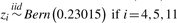		0.09375	0.15
5			L2 = (Z4∧Z5∧Z21∧!Z45)ν	0.10156	0.05
			(Z5∧Z11∧Z21∧!Z45)ν
6			(Z5∧Z16∧Z21∧Z33∧!Z45)	0.10156	0.15
7	Latent predictora		L3 = (Z4∧Z5) ν (Z5∧Z11∧Z21)	0.3125	0.025
8			L4 = (Z4∧Z5∧Z21) ν (Z5∧Z11∧Z21)	0.1875	0.025

For the latent predictor scenario^a, Z₂₁ represents a latent predictor and is not observed in the data used to construct LR, logicFS, and LF models.

We consider sample sizes ranging from 25 to 1000. For each combination of simulation case and sample size, we generate 500 datasets. We evaluate the performance of LR(W), FS(W, B) and LF(W, B) using a test dataset of 100 observations generated in the same way as the training data. For model evaluation, let K (K ⊂ F) be the set of five PIs in LF(W, B) or FS(W, B) with maximum absolute VIMP.LF or VIMP.FS values, respectively. Evaluation criteria are: (i) mean model error rate, defined as the misclassification rate of the fitted model for the test dataset (2); (ii) identification of PIs in L according to VIMP.LR and inclusion in K for LF; and (iii) identification of PIs in L according to subset matching as described in Section 2.3 for LR and according to subset matching to K for LF and logicFS.

We use the LogicReg package (Kooperberg and Ruczinski, 2007) in R v. 2.7.1 (R Development Core Team, 2009) with simulated annealing optimization to fit all LR models. Maximum model size for LR models is selected using the cross-validation procedure suggested by Ruczinski et al. (2003). Cross-validation improves LR model performance by reducing the likelihood of over-fitting. LogicFS models are constructed using the logicFS package (Schwender, 2007) available at www.bioconductor.org. The LF algorithm (Section 2.1) is used to generate all ensemble models. LogicFS and LF models include B = 100 logic regression trees. The same starting and ending annealing temperatures are selected for LR, logicFS and LF. The starting temperature of 2 is selected such that ∼90% of ‘new’ models are accepted. The final temperature of −1 is set to achieve a score where >5% of new models are accepted. The cooling schedule is set so that 50 000 iterations are required to get from start to end temperature. Increasing the number of iterations to 250 000 did not affect our findings. With these settings, an ensemble is constructed in less than a minute on a Windows 2.26 GHz machine.

3.1 Predictor noise

Cases 1 and 2 (Table 1) examine the effects of noisy predictors on LR, logicFS and LF performance. The results for the mean model error rates for samples sizes 25, 200 and 1000 are shown in Table 2. Model error rates are similar at all sample sizes for all three methods for Cases 1 and 2. Figure 1 shows the proportion of times each method recovered the PI X₄ ∧ X₅ using exact and subset matching by sample size for each noise level. Error bars in the figure represent 95% confidence intervals for the proportions.

Table 2.

Mean model error rate for simulation Cases 1–6 (Table 1)

Case	Predictor	Sample	LR mean	logicFS mean	LF mean
	noise (%)	size	error rate	error rate	error rate
1	5	25	0.190	0.190	0.184
		200	0.070	0.060	0.061
		1000	0.062	0.060	0.060
2	15	25	0.320	0.314	0.310
		200	0.200	0.201	0.199
		1000	0.174	0.173	0.173
3	5	25	0.135	0.124	0.104
		200	0.062	0.063	0.064
		1000	0.055	0.048	0.053
4	15	25	0.136	0.127	0.108
		200	0.107	0.103	0.103
		1000	0.102	0.102	0.101
5	5	25	0.130	0.124	0.102
		200	0.081	0.079	0.082
		1000	0.063	0.049	0.080
6	15	25	0.125	0.116	0.105
		200	0.104	0.102	0.100
		1000	0.100	0.098	0.100

Error rate variance ranges between 1.1 × 10⁻⁴ and 1.4 × 10⁻⁷.

Fig. 1.

Recovery of the PI X₄ ∧ X₅ for model L₁ (Cases 1 and 2) in data with 5 or 15% noise in all predictors. N = 500 replications for each sample size. Error bars represent 95% confidence intervals.

Figure 1 shows that LF is significantly more likely to exactly identify the PI X₄ ∧ X₅ than LR for sample sizes n = 25 to 100 in data with 5% noise and for n = 25 to 300 in data with 15% noise. The performance of LF and logicFS is similar in data with 5% noise although LF more frequently exactly identifies the PIs for sample sizes n ≤ 50. LF exactly identifies X₄ ∧ X₅ significantly more frequently than logicFS in data with 15% noise for sample sizes from n = 35 to 200. The results for PI X₅ ∧ X₁₁ were similar to those of X₄ ∧ X₅ (results not shown).

The performance of the three methods does not improve significantly with subset matching in data with 5% noise. However, in data with 15% noise, the ability of all three methods is enhanced under subset matching. Although the performance of LR and logicFS is closer to LF when subset matching is used, LF still identifies the PIs more frequently than logic FS for 50 ≤ n ≤ 150 and more frequently that LR for 25 ≤ n ≤ 300. Both LR and logicFS identify the relationship between X₄ and X₅ and between X₅ and X₁₁, but the tendency is to add spurious components to the PI.

We also consider a null scenario in which there is no association between predictors and the response. The predictors follow the distribution for Cases 1 and 2 (Table 1) and the response is . We simulate 500 datasets for sample sizes ranging from 25 to 1000 and examine the proportion of times each method recovers the PIs X₄ ∧ X₅ and X₅ ∧ X₁₁ according to the criteria defined for these simulations. All three methods recover these PIs in <2% of all simulation runs at all sample sizes.

3.2 Model complexity

Cases 3–6 (Table 1) examine the effect of model complexity on the ability of each method to correctly identify PIs truly associated with the response and on the error rate of the fitted model. Cases 3 and 4 investigate a simple logic expression, L₁, describing the response using two PIs of size 2. Cases 5 and 6 investigate a more complex model, L₂, containing three PIs, two of Size 4 and one of Size 5. These models also have a lower probability of an observed response value of 1 relative to Cases 1 and 2, which has been shown to reduce the ability of LR to identify interactions known to be important (Vermeulen et al., 2007).

Results for average model error rates for sample sizes 25, 200 and 1000 (5 and 15% noise) for Cases 3–6 are shown in Table 2. Figure 2 represents the proportion of times each method recovers L₁'s PI X₄ ∧ X₅, exactly and by subset matching, for 5% predictor noise. Figure 3 represents the proportion of times each method recovers L₂'s PIs X₄ ∧ X₅ ∧ X₂₁ ∧ !X₄₅ and X₅ ∧ X₁₆ ∧ X₂₁ ∧ X₃₃ ∧ !X₄₅ for 5% noise.

Fig. 2.

Recovery of the PI X₄ ∧ X₅ for L₁ (Case 3) with P(L = 1) = 0.09375, in data with 5% noise in all predictors. N = 500 replications for each sample size. Error bars represent 95% confidence intervals.

Fig. 3.

Recovery of the PIs X₄ ∧ X₅ ∧ X₂₁ ∧ !X₄₅ and X₅ ∧ X₁₆ ∧ X₂₁ ∧ X₃₃ ∧ !X₄₅ for the complex model, L₂ (Case 5), in data with 5% noise in all predictors. N = 500 replications for each sample size. Error bars represent 95% confidence intervals.

The mean model error rate of LF is significantly smaller than both LR and logic for n = 25 in Cases 3 through 5. However, logicFS has smaller mean model error rate than LF and LR in Cases 3 and 5 for n ≥ 200. The difference in mean model error rates for logicFS and LF is significant for n ≥ 500 for Case 3 and for n ≥ 300 for Case 5.

From Figure 2, for data with a simple underlying model L₁ and 5% noise in the predictors LF is significantly more likely to exactly identify the true PI, X₄ ∧ X₅, than LR and logicFS for n ≥ 35 and for 35 ≤ n ≤ 500, respectively. The results for recovery of X₅ ∧ X₁₁ are similar in data with 5% predictor noise. In data with 15% noise, LR and logicFS exactly identify these PIs X₄ ∧ X₅ and X₅ ∧ X₁₁ in <5% of models at all sample sizes. However, LF exactly identifies the PIs in >60% of all models once n = 150 (see Fig. 1, Section 1 of the Supplementary Material). A comparison of the performance of both methods for Cases 1 and 2 versus Cases 3 and 4, which consider the same simple model but with P(L₁ = 1) = 0.375 compared with P(L₁ = 1) = 0.09375, respectively, indicate that all three methods are less likely to recover the true PIs if there is reduced probability of a response being 1 (Figs 1 and 2).

In the complex model, L₂, LF and logicFS exactly identify the two PIs of Size 4 with greater frequency than LR at sample sizes n ≥ 150 for both noise levels. LF and logicFS identify all PIs in L₂ equally well with the exception of the two PIs of Size 4 at n = 75 and the largest PI at n = 1000 where logicFS exactly identifies these PIs more frequently than LF. All three methods have difficulty in identifying the largest PI in L₂ (Fig. 3). This is likely due to the fact that the largest PI explains only a small proportion of variation in the response. In data with 15% noise, the proportion of times the two Size 4 PIs are recovered is greatly reduced for all three methods. However, LF exactly identifies the two Size 4 PIs more frequently than LR for n ≥ 150 and than logicFS for n ≥ 300. LF achieves a maximum of 23% of models containing exact matches compared with 15% for logicFS and 2% for LR. In data with 15% noise, none of the methods is able to recover the largest PI exactly.

LR, logicFS and LF all demonstrate improved performance for true underlying model L₁ when evaluated by subset matching. However, LF identifies the two PIs from model L₁ more often than LR and logicFS for sample sizes between n = 75 and n = 200 in data with 5% noise and between n = 75 and n = 300 for data with 15% noise.

Use of subset matching for identifying PIs in the complex model L₂ only significantly improves the performance of the three methods in data with 15% predictor noise (see Fig. 2, Section 1 in the Supplementary Material). LogicFS and LF both identify the PIs of Size 4 more frequently than LR as subset matches for n ≥ 300. LogicFS identifies these two PIs more frequently as subset matches than LF for n ≥ 750. Even using subset matching, all three methods have difficulty identifying the Size 5 PI in the complex model at both noise levels.

3.3 Latent predictors

In Cases 7 and 8 (Table 1), we consider models in which a latent variable directly affects one or more PIs explanatory of the response. The true response for Case 7, L₃, has two PIs but only Z₅ ∧ Z₁₁ ∧ Z₂₁ contains the latent predictor Z₂₁. In Case 8, the response, L₄, has similar PIs and both PIs are affected by the latent predictor.

Corresponding to the latency of Z₂₁, predictor X₂₁ is not observed and therefore not available when constructing the models; thus we cannot identify the true PIs. For these cases, we determine the proportion of times each method identifies X₄ ∧ X₅ and X₅ ∧ X₁₁, the observed components of the true PIs. The mean model error rate was not statistically different at a majority of sample sizes (results not shown). The only exception occurs at n = 25 where LF and logicFS have significantly smaller mean error rates than LR. Figure 4 shows the proportion of times each method recovers the two partial PIs by sample size for L₃.

Fig. 4.

Recovery of exact and subset matches for observed components of the PI X₅ ∧ X₁₁ ∧ X₂₁ for L₃ (Case 7). N = 500 replications for each sample size. Error bars represent 95% confidence intervals.

The ability of each method to recover the partial PIs X₄ ∧ X₅ or X₅ ∧ X₁₁ depends on the model. For L₃, where only the relationship between X₅ and X₁₁ is strongly affected by the absence of X₂₁, X₄ ∧ X₅ is exactly recovered in 100% of models for n > 150 for all three methods, while exact recovery of X₅ ∧ X₁₁ occurs much less frequently (Fig. 4). LF is more adept at exactly recovering X₅ ∧ X₁₁ than LR and logicFS at all sample sizes. LR and logicFS rarely recover the exact PI X₅ ∧ X₁₁ for data generated under L₃ (Fig. 4). In L₄, LR and logicFS rarely exactly recover either PI even with increasing sample size. However, LF is able to exactly identify both PIs in L₄ in up to 60% of models (see Fig. 3, Section 2 in the Supplementary Material).

For X₅ ∧ X₁₁ for L₃ and for both X₄ ∧ X₅ and X₅ ∧ X₁₁ for L₄, the performance of LR and logicFS improves greatly with subset matching. Despite improvement in the performance of LR with subset matching, LF performs significantly better than LR in both models and for all sample sizes n ≥ 35 (Fig. 4). However, logicFS identifies the PI X₅ ∧ X₁₁ in L₃ significantly more frequently as subset matches than LF for sample sizes ranging between n = 75 and n = 200. LogicFS also identifies both PIs in L₄ as subset matches more frequently than LF for n ≥ 500.

4 PERIODONTAL DISEASE IN AFRICAN AMERICANS WITH DIABETES

We examine the association of genetic and health factors with prevalence of generalized adult periodontitis using data from a study conducted at the Center for Oral Health Research at the Medical University of South Carolina. Here, generalized adult periodontitis is defined as ≥3 mm clinical attachment loss and >30% of sites affected.

These data are drawn from 244 African American adults with diabetes. Information on each subject includes the binary health indicators total cholesterol (> 200 mg/dl), HDL (> 40 mg/dl), triglycerides (> 150 mg/dl), C-reactive protein levels (> 1 mg/l), HbA1c levels (> 7%), smoking status (current versus former and never, former versus current and never) and genotype data for nine single nucleotide polymorphisms (SNPs) believed to play a role in inflammation and/or bone resorption. Among the 244 participants in the study, 95 have generalized adult periodontitis.

Seven of the SNPs are coded by two dummy variables for the LF analysis. The first dummy variable takes value 1 if the subject has a SNP genotype with at least one copy of the minor allele (dominant effect of the minor allele) and the second takes value 1 if the subject has two copies of the minor allele (recessive effect of the minor allele). This coding allows for consideration of both dominant and recessive genetic effects in the model. The remaining two SNPs for which no subjects have two copies of the minor allele are coded for the dominant genetic effect only. The final dataset includes 23 binary predictors composed of these 16 SNP dummy variables and seven health indicators.

Two LF models, each with B = 100 trees, are constructed from the data. The first LF model includes all SNPs and health indicators as predictors. The second model is constructed with only the SNPs as predictors. The top five PIs for both models, as determined by VIMP.LF magnitude, are shown in Figure 5. VIMP.LF scores are normalized so the largest is 1. The most important single predictor identified by the models is the recessive genetic effect for the IL-1α⁻⁸⁸⁹ minor allele (IL1A1.22). Previous studies suggest that the minor allele of IL-1α⁻⁸⁸⁹ is associated with advanced periodontitis, though these studies considered only the dominant genetic effect (Gore et al., 1998; Kornman et al., 1997; Moreira et al., 2007). Also two PIs selected among the top five by VIMP.LF magnitude appear in both models: (i) IL1B.12 ∧ IL1A1.22 and (ii) IL1A1.22 ∧ !MMP3.12 (Fig. 5). IL1A1.22 represents the recessive genetic effect for the IL-1α⁻⁸⁸⁹ minor allele, IL1B.12 represents the dominant genetic effect for the IL-1β⁺³⁹⁵⁴ minor allele and !MMP3.12 represents the recessive genetic effect for the MMP3 major allele. PI(a), IL1B.12 ∧ IL1A1.22, suggests an association consistent with previous reports (Gore et al., 1998; Kornman et al., 1997). The recessive genetic effect for the MMP3 minor allele is implicated in chronic periodontitis in a Brazilian population (Astolfi et al., 2006), but the interaction described by PI(b) has not been noted previously.

Fig. 5.

Normalized VIMP.LF for model including SNPs and health indicators (LF1) and model including only SNPs (LF2).

5 CONCLUSIONS

LR has the ability to model complex interactions such as those that might describe a disease state. To improve identification of important PIs, Schwender and Ickstadt (2008) presented a bagged version of LR called logicFS. Unlike their approach, our method randomly selects a maximum size when building each tree in the ensemble, thereby enhancing the probability that the forest will discover smaller PIs. We also introduce a permutation measure to quantify PI importance. Additionally, we present the notion of subset matching to enhance sensitivity to PI contributions. We extend simulations in previous studies evaluating the performance of LR, logicFS and our ensemble of LR trees, LF, by including larger sample sizes, noise in the predictors and smaller probabilities of the response variable taking value 1. Our results show that LF and logicFS are better able identify important PIs than LR. LF also demonstrates improved ability to recover PIs relative to logicFS at smaller sample sizes in a majority of the simulation scenarios. We also show that forced inclusion of smaller trees in the forest is beneficial for PI identification, particularly in data with latent variables or noisy predictors.

Using the permutation-based measure of variable importance, LF is more adept at identifying informative PIs in noisy data, in data with a latent variable and in more complex true models than LR and logicFS. The greatest improvement from LF occurs in scenarios where PIs are smaller and more weakly associated with a response or in situations where there is failure to observe a predictor truly associated with the response. LF also exhibits greater improvement relative to LR as sample size increases, while the largest improvements in performance of LF relative to logicFS occurs at smaller sample sizes (35 ≤ n ≤ 200). The main exception occurs for data following a complex underlying model where the performance of LF and logicFS is similar for recovery of the three PIs in L₂ (Fig. 3). LR, logicFS and LF all demonstrate limited ability to recover large PIs weakly associated with the outcome in the presence of smaller PIs with stronger associations.

We also introduce the idea of subset matching. If a PI persists in increasingly larger PIs, then that PI may represent a true association. For example, discovery of the PIs P, P ∧ Q₁ and P ∧ Q₂ ∧ Q₃ suggests a true association of the PI P with the response. In LF, as opposed to LR, we have the richness of the forest in which to evaluate this persistence of predictors and PIs. Especially in a latent variable setting, where not all components of a predictive PI are observed, persistence throughout the forest facilitates identification of the observed components of that PI.

LF, LR and logicFS were also compared with Random Forest (RF) and MCLR. The mean model error rate for RF was larger than all three methods for a majority of sample sizes for simulation Cases 1, 2, 3, 5 and 7 and comparable with LF for Cases 4 and 8. RF is designed to identify important individual predictors from among all predictors in the data and concerning identification of individual predictors, RF performed comparably with LF. However, RF provides no direct mechanism for quantifying associations among predictor interactions and response. MCLR is designed to identify predictors that co-occur with the greatest frequency. MCLR identified predictor combinations from true PIs in <5% of all models for all simulation scenarios (results are not shown).

The simulations presented in this article are by no means an exhaustive study of all scenarios one might encounter in biologic data. However, this study provides insight into the effectiveness of ensemble methods, LF in particular, in improving the identification of PIs in scenarios likely in biological studies. LF is not designed to handle data with a larger number of predictors than observations. Based on simulations examining the performance of LF, data should have at least twice as many observations as predictors for the best performance.

The methods and measures presented in this study were restricted to classification trees. LR has the ability to build trees as predictors in linear and logistic regression models by altering the scoring functions used in constructing the LR model (sums of squares and deviance, respectively). Further studies are necessary to assess the performance of LF with such alternative scoring functions.

REFERENCES

- Alvarez-Castro JM, Carlborg O. A unified model for functional and statistical epistasis and its application in quantitative trait loci analysis. Genetics. 2007;176:1151–1167. doi: 10.1534/genetics.106.067348. [DOI] [PMC free article] [PubMed] [Google Scholar]
- Astolfi CM, et al. Genetic polymorphisms in the MMP-1 and MMP-3 gene may contribute to chronic periodontitis in a brazilian population. J. Clin. Periodontol. 2006;33:699–703. doi: 10.1111/j.1600-051X.2006.00979.x. [DOI] [PubMed] [Google Scholar]
- Austin PC. A comparison of regression trees, logistic regression, generalized additive models, and multivariate adaptive regression splines for predicting AMI mortality. Stat. Med. 2007;26:2937–2957. doi: 10.1002/sim.2770. [DOI] [PubMed] [Google Scholar]
- Breiman L. Bagging Predictors. Mach. Learn. 1996;24:123–140. [Google Scholar]
- Carlborg O, Haley CS. Epistasis: too often neglected in complex trait studies? Nat. Rev. Genet. 2004;5:618–625. doi: 10.1038/nrg1407. [DOI] [PubMed] [Google Scholar]
- Dietterich TG. An experimental comparison of three methods for constructing ensembles of decision trees: bagging, boosting, and randomization. Mach. Learn. 2000;40:139–157. [Google Scholar]
- Etzioni R, et al. Combining biomarkers to detect disease with application to prostate cancer. Biostatistics. 2003;4:523–538. doi: 10.1093/biostatistics/4.4.523. [DOI] [PubMed] [Google Scholar]
- Etzioni R, et al. Prostate-specific antigen and free prostate-specific antigen in the early detection of prostate cancer: do combination tests improve detection? Cancer Epidemiol. Biomarkers Prev. 2004;13:1640–1645. [PubMed] [Google Scholar]
- Fleisher H, et al. Exclusive-OR representation of Boolean functions. IBM J. Res. Dev. 1983;27:412–416. [Google Scholar]
- Friedman J. Greedy function approximation: a gradient boosting machine. Ann. Stat. 2001;29:1189–1202. [Google Scholar]
- Gore EA, et al. Interleukin-1β+3953allele 2: association with disease status in adult periodontitis. J. Clin. Periodontol. 1998;25:781–785. doi: 10.1111/j.1600-051x.1998.tb02370.x. [DOI] [PubMed] [Google Scholar]
- Janes H, et al. Identifying target populations for screening or not screening using logic regression. Stat. Med. 2005;24:1321–1338. doi: 10.1002/sim.2021. [DOI] [PubMed] [Google Scholar]
- Keles S, et al. Regulatory motif finding by logic regression. Bioinformatics. 2004;20:2799–2811. doi: 10.1093/bioinformatics/bth333. [DOI] [PubMed] [Google Scholar]
- Kooperberg C, Ruczinski I. Identifying interacting SNPs using Monte Carlo logic regression. Genet. Epidemiol. 2005;28:157–170. doi: 10.1002/gepi.20042. [DOI] [PubMed] [Google Scholar]
- Kooperberg C, Ruczinski I. LogicReg: Logic Regression. 2007 R package version 1.4.9. Available at: http://cran.r-project.org/ (last accessed date April 4, 2010) [Google Scholar]
- Kooperberg C, et al. Logic regression for analysis of the association between genetic variation in the renin-angiotensin system and myocardial infarction or stroke. Am. J. Epidemiol. 2007;165:334–343. doi: 10.1093/aje/kwk006. [DOI] [PubMed] [Google Scholar]
- Kornman KS, et al. The interleukin-1 genotype as a severity factor in adult periodontal disease. J. Clin. Periodontol. 1997;24:72–77. doi: 10.1111/j.1600-051x.1997.tb01187.x. [DOI] [PubMed] [Google Scholar]
- Kotti S, et al. Strategy for detecting susceptibility genes with weak or no marginal effects. Hum. Hered. 2007;63:85–92. doi: 10.1159/000099180. [DOI] [PubMed] [Google Scholar]
- Kumar S, et al. Biomarkers in cancer screening, research and detection: present and future: a review. Biomarkers. 2006;11:385–405. doi: 10.1080/13547500600775011. [DOI] [PubMed] [Google Scholar]
- Lo SH, Zhang T. Backward haplotype transmission association (BHTA) algorithm - a fast multiple-marker screening method. Hum. Hered. 2002;53:197–215. doi: 10.1159/000066194. [DOI] [PubMed] [Google Scholar]
- Manne U, et al. Recent advances in biomarkers for cancer diagnosis and treatment. Drug Discov. Today. 2005;10:965–976. doi: 10.1016/S1359-6446(05)03487-2. [DOI] [PubMed] [Google Scholar]
- Moreira PR, et al. The IL-1α−889gene polymorphism is associated with chronic periodontal disease in a sample of brazilian individuals. J. Periodont. Res. 2007;42:23–30. doi: 10.1111/j.1600-0765.2006.00910.x. [DOI] [PubMed] [Google Scholar]
- Negm RS, et al. The promise of biomarkers in cancer screening and detection. Trends Mol. Med. 2002;8:288–293. doi: 10.1016/s1471-4914(02)02353-5. [DOI] [PubMed] [Google Scholar]
- Ruczinski I, et al. Logic regression. J. Comput. Graph. Stat. 2003;12:475–511. [Google Scholar]
- R Development Core Team. R Foundation for Statistical Computing. Vienna, Austria: 2009. R: A language and environment for statistical computing. Available at: http://www.r-project.org (last accessed date April 4, 2010) [Google Scholar]
- Schwender H, Ickstadt K. Identification of SNP interactions using logic regression. Biostatistics. 2008;9:187–198. doi: 10.1093/biostatistics/kxm024. [DOI] [PubMed] [Google Scholar]
- Schwender H. logicFS: Identifying interesting SNP interactions with logicFS. Bioconductor package. 2007 [Google Scholar]
- Srivastava S. Cancer biomarkers: an emerging means of detecting, diagnosing and treating cancer. Cancer Biomark. 2005;1:1–2. [PubMed] [Google Scholar]
- Vermeulen SH, et al. Application of multi-locus analytical methods to identify interacting loci in case-control studies. Ann. Hum. Genet. 2007;71:689–700. doi: 10.1111/j.1469-1809.2007.00360.x. [DOI] [PubMed] [Google Scholar]
- Wagner PD, et al. Challenges for biomarkers in cancer detection. Ann. N. Y. Acad. Sci. 2004;1022:9–16. doi: 10.1196/annals.1318.003. [DOI] [PubMed] [Google Scholar]
- Zethelius B. Use of multiple biomarkers to improve the prediction of death from cardiovascular causes. N. Engl. J. Med. 2008;358:2107–2116. doi: 10.1056/NEJMoa0707064. [DOI] [PubMed] [Google Scholar]
Associated Data
This section collects any data citations, data availability statements, or supplementary materials included in this article.