Spatial misalignment in time series studies of air pollution and health data

Abstract

Time series studies of environmental exposures often involve comparing daily changes in a toxicant measured at a point in space with daily changes in an aggregate measure of health. Spatial misalignment of the exposure and response variables can bias the estimation of health risk, and the magnitude of this bias depends on the spatial variation of the exposure of interest. In air pollution epidemiology, there is an increasing focus on estimating the health effects of the chemical components of particulate matter (PM). One issue that is raised by this new focus is the spatial misalignment error introduced by the lack of spatial homogeneity in many of the PM components. Current approaches to estimating short-term health risks via time series modeling do not take into account the spatial properties of the chemical components and therefore could result in biased estimation of those risks. We present a spatial–temporal statistical model for quantifying spatial misalignment error and show how adjusted health risk estimates can be obtained using a regression calibration approach and a 2-stage Bayesian model. We apply our methods to a database containing information on hospital admissions, air pollution, and weather for 20 large urban counties in the United States.

1. INTRODUCTION

Estimating the health risks of environmental exposures often involves examining data at different levels of spatial resolution. This mismatch between data measured at different resolutions results in spatial misalignment (Banerjee and others, 2004), which can induce error and bias estimates of risk. Spatial misalignment in environmental health studies is common because the exposure data and the health data often come from independent sources. For example, in an air pollution study in the United States, data on ambient air pollution levels often are based on a network of monitors operated by the US Environmental Protection Agency (EPA) where each monitor measures pollution at a specific point location. Data on an outcome of interest, such as the numbers of hospital admissions for cardiovascular disease, might come from the Centers for Medicare and Medicaid Services. In cohort studies that compare health outcomes and exposures across people, information about individual persons may be available but exposure data may be derived from a computer model at a much lower resolution. Because health and exposure data are often collected independently of each other, they are rarely spatially aligned. Hence, a direct comparison of the exposure and health outcome is not possible without a model (or an assumption) to align the 2 in the spatial domain.

In a time series study of air pollution and health, one is interested in estimating associations between daily changes in county-wide hospital admissions or mortality counts and daily changes in county-wide average levels of a specific pollutant. The problem is that we do not directly observe county-wide average pollutant levels. Rather, we have measurements taken at a handful of monitors (sometimes only one) located inside the county boundaries. For a spatially homogeneous pollutant, the value of the pollutant at a single monitor can be representative of the county-wide average ambient level of that pollutant. Some pollutants, particularly some gases such as ozone, are reasonably spatially homogeneous across the area of a county. The total mass of particulate matter (PM) less than 2.5 μm in aerodynamic diameter (PM_2.5), whose health risks have been examined extensively, is fairly spatially homogeneous, and monitor measurements of PM_2.5 in counties with multiple monitors tend to be highly correlated across both time and space (Peng and others, 2008; Bell and others, 2007). With a pollutant such as PM_2.5, the misalignment between the continuous nature of the pollutant process and the aggregated nature of the health data does not typically pose as serious a problem as some other pollutants. In this situation, current approaches for data analysis may provide reasonable estimates of risk.

There are many sources of measurement error in the analysis of air pollution and health data, and much previous work has focused on the mismatch between personal and ambient exposures to an airborne pollutant (Dominici and others, 2000; Zeger and others, 2000). This is indeed an important problem, but it is typically not the one that can be dealt with using the types of data that are routinely available. Given an aggregated health outcome, the ideal exposure is the average “personal” exposure over the population (Zeger and others, 2000). Because it is unrealistic to measure this quantity repeatedly over long periods of time, population studies must resort to suitable proxies such as the average “ambient” concentration.

A key assumption made in previous time series analyses of air pollution and health data was that the pollutant of interest is spatially homogeneous and that the monitor value on a given day (or the average of a few monitors) is approximately equal to the true ambient average concentration over the study population area. Any difference between the monitor value and the true ambient average concentration is what we call “spatial misalignment error.” In past analyses, the assumption that this error was zero may have been reasonable given that most previous analyses focused on pollutants such as the total mass of particulate matter (PM₁₀, PM_2.5), ozone, and other pollutants that have been shown to be fairly spatially homogeneous over relatively long distances (Samet, Zeger, and others, 2000).

Recently, data have become available from the US EPA's Chemical Speciation Trends Network (STN) as well as State and Local Air Monitoring Stations which provide daily mass concentrations of approximately 60 different chemical elements of PM_2.5. These data are monitored in over 200 locations around the United States starting from the year 2000. Although the data are promising and are the subject of intense interest and new research, they also raise new statistical challenges. In particular, the usual assumption that the monitor value is approximately equal to the ambient average is less tenable when examining certain components of PM_2.5 (Bell and others, 2007). Figure 1 shows the correlations between pairs of monitors in the STN for 7 components of PM_2.5 mass as a function of the distance between the monitors. For all the chemical components, the correlations decrease with distance, but the rate at which the correlations decrease varies by component. Figure 1 provides evidence that some components of PM_2.5 are spatially homogeneous with high correlations over long distances (≥50 km), while other components are spatially heterogeneous and exhibit practically no correlation beyond short distances (<20 km).

Fig. 1.

Correlations between monitor pairs as a function of distance between monitors (correlations are plotted on the Fisher's z-transform scale).

Much of the spatial heterogeneity in the chemical components measured by the STN can be explained by the nature of the sources of the various components. For example, elemental carbon (EC) and organic carbon matter (OCM) tend to be emitted primarily from vehicle or other mobile sources, and thus their spatial distribution can depend on the localized nature of those sources. Secondary pollutants such as sulfate and nitrate are created in the air by the chemical and physical transformation of other pollutants and tend to be more regional in nature. Hence, for spatially heterogeneous pollutants such as EC or OCM, the daily level of those pollutants at a single monitor may be a poor surrogate for the daily county-wide average ambient level of that pollutant.

Although we focus mainly on time series studies in this paper, spatial misalignment can also induce error in cross-sectional studies of air pollution and health. Gryparis and others (2008) demonstrate in detail how to handle the misalignment errors in these types of studies and compare the performance of a number of different statistical approaches. An alternate modeling approach has been proposed by Fuentes and others (2006) for estimating the spatial association between speciated fine particles and mortality. Both approaches introduce a spatial model for the monitored pollutant concentrations and either predict pollutant values at unobserved locations or compute area averages over counties to link with county-level health data. While much work has been done illustrating the problem of spatial misalignment for cross-sectional studies, little has been done for time series studies estimating short-term health effects.

With the emergence of the PM components data and the critical interest in estimating the health effects of those components, the problem of spatial misalignment becomes relevant and new statistical methods need to be developed to properly analyze these data. Specifically, there is a need to develop approaches that account for the varying amounts of spatial information we have about chemical component levels over wide regions. These methods could be used to estimate and report health risks associated with PM components while simultaneously incorporating the spatial information (or lack thereof) we have for each component.

In this paper, we describe a general method for estimating health risks associated with PM components from time series models while adjusting for potential spatial misalignment error. We first develop a spatial–temporal model for the exposure of interest and estimate the degree of spatial misalignment error for each component in a location. We then apply 2 methods—a regression calibration procedure and a 2-stage Bayesian model—to estimate the health risks associated with these components and compare the results to standard approaches. Our methods are applied to a large database containing information on daily hospital admissions for cardiovascular diseases and chemical components of ambient PM for 20 large urban counties in the United States.

2. CURRENT METHODS

Current approaches to time series analysis of air pollution and health data typically use county-level health data and treat the day as the temporal unit of analysis. On a given day, the outcome is the count of the number of hospitalizations for a specific disease occurring in that county or perhaps the number of deaths due to a specific cause. The exposure is typically the level of a pollutant recorded at a monitor located within the county boundaries on that day. If there are multiple monitors located in the county (sometimes between 2 and 10), then an average of the available monitors on that day is used as a single exposure concentration. For example, in the National Mortality, Morbidity, and Air Pollution Study (NMMAPS), multiple monitors were averaged using a 10% trimmed mean to remove any outlying large or small values (Samet, Dominici, and others, 2000). Similar approaches have been taken in other time series studies (Katsouyanni and others, 2001).

For a given county, there is a time series for the outcome Y_t and a single time series for the exposure pollutant which might represent the daily averages across multiple monitors. Generalized additive models are often used to estimate the day-to-day association between the 2 time series while controlling for the potential confounding effects of weather, season, and other factors (Peng and others, 2006: Welty and Zeger, 2005; Touloumi and others, 2004). Log-linear Poisson models are commonly used with smooth functions of time, temperature, and dew point temperature (or relative humidity),

(2.1)

where Y_t is the count of the number of events (i.e. admissions, deaths), ${\mathbf{z}}_t$ represents a vector of covariates (e.g. indicators for the day of the week, age category–specific intercepts), s is a smooth function, and the ${\lambda }_i$s are smoothing parameters controlling the smoothness of their respective functions. Common choices for the smooth functions include penalized splines, smoothing splines, and parametric natural splines. Variations on the model in (2.1) are used depending on meteorological or other local conditions. In addition, it is common to use a quasi-likelihood approach rather than a fully Poisson model to allow for overdispersion.

The parameter of interest is θ, the log–relative risk of the exposure , with the remaining elements of the model being nuisance parameters. When total mass PM is the exposure of interest, the risk is often reported as $100\times \left(\text{exp}\right(10\theta )-1)$, which is the percent increase in the outcome for a 10 μg/m³ increase in PM. Another common increment for reporting risk estimates is the interquartile range of the pollutant data.

One key assumption made by current approaches is that the monitor value (or average of monitor values) represents the average ambient concentration. For some pollutants such as PM_2.5 total mass, this assumption is approximately true. However, for many components of PM_2.5, the observed spatial heterogeneity of the component raise concerns about whether the monitor values are good surrogates for the average ambient concentration.

In Section 3, we present a model for assessing the degree of spatial misalignment measurement error when using PM chemical components data and an approach for adjusting estimates of the short-term health risks of PM chemical components obtained from time series regression models.

3. STATISTICAL MODEL FOR SPATIAL MISALIGNMENT

Our approach to estimating the short-term health risks of chemical components of PM_2.5 while adjusting for spatial misalignment error is divided into 2 parts.

1. Spatial–temporal model: The first part of our approach fits a spatial–temporal model to the pollutant data using all available data from the national monitoring network. Once this global model is fitted, we can use it to make predictions in specific counties around the country (Section 3.1).

2. Health risk model: The second part of our approach involves health risk estimation for residents of a specific US county. This part connects the health data for a given county with the pollutant data via the spatial–temporal model. The outcome is the number of adverse events (e.g. hospital admissions) occurring in the county on a given day. The exposure is the ambient average pollutant level in that county which we estimate by integrating the spatial–temporal model over the area determined by the county's geographic boundaries (Section 3.4).

In this paper, we take each pollutant separately and fit a separate spatial–temporal model to each pollutant. Once we have a spatial–temporal model for a given pollutant, we can connect the model to health data from a county to estimate health risks in that county. To estimate health risks for the same pollutant in a different county, we use the same spatial–temporal model for that pollutant and change the health risk model to incorporate health data from the new county. Similarly, we estimate a new exposure by integrating the spatial–temporal model over the area defined by the new county's geographic boundaries. Table 1 summarizes the different modeling components and the data used to fit each part of the model.

Table 1.

Model components and data sets used to estimate parameters

Model component	Data	Parameters
Spatial–temporal	National speciation monitoring network: 313 monitors with 1-in-6 day observations on PM2.5 chemical components, years 2000–2006 (see Figure 2 for locations of monitors)	μ(), ϕ, κ, σ, x
Health risk	Daily county-specific time series of cardiovascular hospital admissions from Medicare claims, 2000–2006; county-specific geographic boundaries; predictions from spatial–temporal model	θ
Spatial misalignment variance	National speciation monitoring network; county-specific geographic boundaries	τ2

A third and separate component of our modeling framework is the spatial misalignment error model. In Sections 3.2–3.3, we employ a classical measurement error model to estimate the proportion of the total temporal variation in the pollutant data that can be attributed to spatial misalignment. Using this approach, we can assess what factors, such as pollutant characteristics, monitoring density, and county size, are associated with spatial misalignment error.

3.1. Spatial–temporal model for exposure

We assume that for a given time t and point location s, a pollutant can be modeled by a spatial stochastic process

where $\mu (\mathbf{s},t)$ is a fixed-effect term and $\epsilon (\mathbf{s},t)$ is a mean zero Gaussian process with variance σ² and correlation function $\rho (·,·)$. We further assume an isotropic covariance model so that

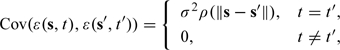where $\Vert ·\Vert$ is the Euclidean distance between 2 points. In this formulation, we do not model the temporal correlation structure and assume that the data are independent in time conditional on the fixed effect $\mu (\mathbf{s},t)$, which may contain nonparametric smoothers of time and/or space. Given that the data in which we are most interested are sampled only once every 6 days, we expect the residual autocorrelation to be small. For the correlation function ρ, we use the flexible Matérn correlation function with parameters ϕ and κ, which has the form

for ϕ > 0 and $\kappa >0$, where 𝒦 is the modified Bessel function of the third kind. We make use of the geoR R package implementation of this model (Ribeiro and Diggle, 2001).

Let ${\mathbf{w}}_t=\left(w\right({\mathbf{s}}_1,t),\dots ,w({\mathbf{s}}_n,t\left)\right)$ and ${\mathbf{\mu }}_t=\left(\mu \right({\mathbf{s}}_1,t),\dots ,\mu ({\mathbf{s}}_n,t\left)\right)$, where ${\mathbf{s}}_1,\dots ,{\mathbf{s}}_n$ are the locations of all the monitors in the pollutant monitoring network. Then for a given time point t, the observed data at that time point follow the distribution ${\mathbf{w}}_t\sim 𝒩({\mathbf{\mu }}_t,{\sigma }^{2}H(\varphi ,\kappa ))$, where H is an n × n correlation matrix with elements

(3.2)

and ρ is the Matérn correlation function. The joint likelihood for the data across all time points is then

(3.3)

where the matrix $H(\varphi ,\kappa )$ is defined as in (3.2). The likelihood in (3.3) can be maximized using standard nonlinear optimization techniques to obtain the maximum likelihood estimates for the parameters σ, ϕ, and κ as well as any parameters incorporated into μ_t. To obtain standard error estimates, we use the diagonal of the inverse Hessian matrix calculated at the maximum (Nocedal and Wright, 1999).

3.2. Spatial misalignment error model

On a given day t, a monitor in a county can be thought of as providing a surrogate measurement for the county-wide average ambient concentration (for now assume that there is only one monitor located in the county). We call this observed monitor value , which is the concentration of the component on day t at the monitor location. Let x_t be the true but unobserved county-wide average concentration of the pollutant on day t. The difference between the 2 values can be described with a classical measurement error model, so that

(3.4)

where u_t is a random variable with $𝔼[u_t]={\eta }_t$ and $\text{Var}(u_t)={\tau }_u^2$. The extent to which differs from x_t is the spatial misalignment error, and τ_u² is the error variance. In practice, we occasionally have more than one monitor in a county, so that reflects the average of the available monitors on day t. As the number of monitors increases, we would expect τ_u² to decrease. Note that the nonzero mean η_t for u_t arises from the inclusion of fixed effects $\mu (\mathbf{s},t)$ in the spatial–temporal model for the pollutant $w(\mathbf{s},t)$. If desired, this could be removed by first detrending all the data but it plays no role in our analysis.

If a pollutant is inherently spatially homogeneous, then τ_u² will likely be small and will generally serve as a good surrogate for the true county-wide average x_t, even with just a single monitor. If the pollutant is inherently spatially heterogeneous, then τ_u² will likely be large and serves as a poor surrogate for the county-wide average. PM components such as EC and silicon, as well as the coarse fraction of PM, tend to fall into this latter category.

The classical measurement error model appears appropriate for this situation because we would expect pollutant values at an individual monitor to be more variable over time than the county-wide average. The other assumption made by the classical model is that the errors are independent of x_t. We will examine this assumption further in the data analysis. Ultimately, it may be that neither the classical nor the Berkson model truly describes the relationship between the observed data and the underlying county-wide average, but the classical model seems reasonable in this application.

Given that a single monitor value can be a poor surrogate for the county-wide average ambient concentration, our goal is to use information from other monitors in neighboring counties to obtain a better estimate of the county-wide average. With a spatial–temporal model for the underlying pollutant process, we can estimate the county-wide average concentration on each day and subsequently use those estimated concentrations to obtain health risk estimates for the pollutant.

3.3. Estimating misalignment error

In this section, we describe how one can estimate τ_u², the spatial misalignment error variance for a specific area. Clearly, if we only had data from a single county with a single monitor, it would not be possible to estimate τ_u² because we require an estimate of x_t, the ambient average. Our approach uses the spatial–temporal model described in Section 3.1 to estimate x_t in a specific county. Because the model is fitted to data from the entire monitoring network, it borrows information from all locations to make predictions in a specific county. The estimate of x_t produced by the spatial–temporal model can subsequently be used to estimate τ_u² for a county.

Suppose we have a county represented by polygon A with monitors located at coordinates ${\mathbf{v}}_1,\dots ,{\mathbf{v}}_m$ within the county boundaries. Then

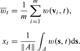Note that the locations ${\mathbf{v}}_1,\dots ,{\mathbf{v}}_m$ will be a subset of all the locations ${\mathbf{s}}_1,\dots ,{\mathbf{s}}_n$ in the national monitoring network used to fit the spatial–temporal model for $w(\mathbf{s},t)$ above.

In a typical air pollution application, the number of monitors m in a county might range from 1 to 10. One intermediate target of inference is the misalignment error variance for a given county. The monitor values inside the county $w({\mathbf{v}}_1,t),\dots ,w({\mathbf{v}}_m,t)$ and the true county-wide average x_t have a joint Normal distribution

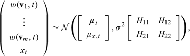(3.5)

where

and

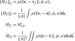The spatial misalignment error variance τ_u² for the county can then be calculated as

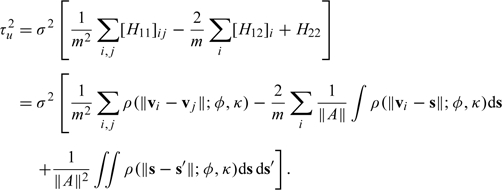The values of σ², ϕ, and κ are unknown, and so we plug in the maximum likelihood estimates of those parameters to obtain our estimate of τ_u². Because the integrals required above are all over the domain of the county boundary, which is likely to be highly irregular, we use a Monte Carlo approximation. We generate random variables $p_1,p_2,\dots ,p_B$ that have a uniform distribution over the area A and then calculate

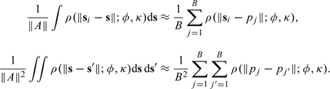These approximations can be made arbitrarily precise by increasing the number of sample points B.

The estimate of τ_u², the spatial misalignment error variance, describes the amount of total variation in the monitoring data for a county (i.e. ) that can be attributable to spatial misalignment error. Note that for the purposes of risk estimation (described in Section 3.4), the explicit calculation of τ_u² is not required. However, the values of τ_u² can be used to assess the impact of spatial misalignment across different counties and different pollutants. The magnitude of τ_u² in a county will depend on the spatial characteristics of the pollutant, the size of the county, and the number of monitors in the county.

3.4. Risk estimation

For the purpose of risk estimation, we need to produce an estimate of the ambient average pollutant level that can be used as the exposure in the health risk model. In this section, we use the spatial–temporal model to estimate the ambient average and present 2 methods for linking the exposure estimate to the health outcome.

Let ${\mathbf{w}}_t=\left(w\right({\mathbf{s}}_1,t),\dots ,w({\mathbf{s}}_n,t\left)\right)$ represent the observed data for all the monitors on day t. Using the spatial–temporal model and the joint distribution in (3.5), the conditional distribution of the true unobserved county-wide average x_t given the data is

(3.6)

where maximum likelihood estimates of σ², ϕ, and κ are plugged in where necessary. We use this conditional distribution to adjust estimates from health risk models in 2 different ways.

Two-stage Bayesian model.

The main approach we describe for adjusting risk estimates for spatial misalignment error is a 2-stage Bayesian model. In the first stage, we estimate $r(x_t|{\mathbf{w}}_t)$, which is simply the distribution in (3.6), that is, the posterior distribution of x_t given the data ${\mathbf{w}}_t$ for each t. The second stage uses $r(x_t|{\mathbf{w}}_t)$ as an informative prior for x_t and estimates the joint posterior distribution of θ and $\mathbf{x}=(x_1,\dots ,x_T)$, given the health data y and the observed pollutant data w,

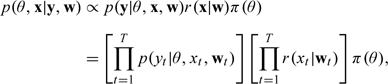where $\mathbf{y}=(y_1,\dots ,y_T)$, $\mathbf{w}=({\mathbf{w}}_1,\dots ,{\mathbf{w}}_T)$, and $\pi \left(\theta \right)$ is a diffuse prior distribution. The likelihood terms $p(y_t|\theta ,x_t,{\mathbf{w}}_t)$ represent the Poisson likelihood used for the time series model relating pollutant exposure to health outcomes. Details on that part of the model are shown in Section 5.2. Note that only the second stage of the model (the health risk estimation) is Bayesian, while the first stage of the model is estimated with maximum likelihood and is considered a fixed prior in the second stage. For a full Bayesian model, the target marginal posterior of θ given the data is

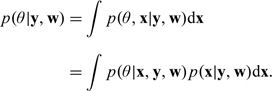Our 2-stage approach effectively assumes that $p\left(\mathbf{x}\right|\mathbf{y},\mathbf{w})\approx r(\mathbf{x}\left|\mathbf{w}\right)$, thus cutting the feedback between x and y. Given that previous studies have indicated that the relationship between the health outcome y and the pollutant exposure x is generally weak, this assumption is not likely to be unreasonable. Furthermore, we obtain the tremendous practical advantage of separating the model into 2 stages so that the substantial work of fitting the spatial model in the first stage (as well as the model checking) can be conducted separately from the parameter estimation in the second stage.

The posterior distribution of θ given the data can be sampled using Markov chain Monte Carlo (MCMC) techniques. Specifically, we use a hybrid Gibbs sampler and alternate sampling from the full conditional distributions of x and θ. Details of the sampling algorithm can be found in the Appendix.

Regression calibration.

As an alternative to the 2-stage Bayesian model, we can use a regression calibration type of approach (Carroll and others, 2006). Using the distribution in (3.6), we can calculate $𝔼[x_t|{\mathbf{w}}_t]$ for each day t. Then substituting $𝔼[x_t|{\mathbf{w}}_t]$ in place of and conducting the standard analysis described in Section 2 would give us the regression calibrated estimate of our risk parameter θ. This method should produce estimates that are similar to the 2-stage model and has the advantage that it requires substantially less computation.

4. SIMULATION STUDY

We designed a simulation study to assess the properties of the regression calibration and 2-stage Bayesian methods. The full details of the simulation design can be found in the supplementary material (available at Biostatistics online). Briefly, we simulated 3 spatial–temporal processes of varying smoothness (rough, moderate, and smooth) and applied the regression calibration and 2-stage Bayesian approaches to the simulated data. The 2 approaches were compared with using the true ambient average pollutant level and the naive approach. Comparisons were made based on coverage of a 95% confidence interval, relative bias, and root mean squared error (RMSE). For the rough pollutant data scenario, there was a clear bias–variance trade-off between the regression calibration and 2-stage model compared to the naive method which just uses the raw mean of the within-county monitors. Both the regression calibration and the 2-stage models appeared reasonably unbiased across the simulations but estimated the log–relative risk parameter with much greater variability. The naive method was quite precise but was biased toward the null. Under the moderate smoothness scenario, all 3 methods did reasonably well with some bias incurred by the naive method. For the smooth scenario, all methods performed equally well.

5. APPLICATION

Daily counts of hospital admissions for the period 2000–2006 were obtained from billing claims of enrollees in the US Medicare system. Each billing claim contains the date of service, disease classification (International Classification of Diseases 9th Revision [ICD-9] codes), age, and county of residence. We considered as an outcome urgent or emergency hospital admissions for cardiovascular diseases, which were calculated using ICD-9 codes (Dominici and others, 2006). The daily counts of hospitalizations were calculated by summing the hospital admissions for each disease of interest recorded as a primary diagnosis. To calculate daily hospitalization rates, we constructed a parallel time series of the numbers of individuals enrolled in Medicare that were at risk in each county on each day. We restricted the analysis to the 20 large counties in the country with at least 100 observations on components of PM_2.5 over the 7-year period of 2000–2006.

In the United States, chemical components of PM_2.5 are typically measured once every 6 days and patterns of missing data vary depending on when monitors began collecting data regularly. For this analysis, we do not attempt to impute the data and only use the days for which we have observations for all relevant variables. Our analysis was limited to the components making up a large fraction of the total PM_2.5 mass or covarying with total mass. These components were sulfate, nitrate, silicon, EC, OCM, sodium ion, and ammonium ion. These 7 components, in aggregate, constituted 83% of the total PM_2.5 mass, whereas all other components individually contributed less than 1% (Bell and others, 2007). In total, we obtained data from 313 chemical speciation monitors across the United States. A map of the monitor locations is shown in Figure 2. National temperature and dew point temperature data were obtained from the National Climatic Data Center on the Earth-Info CD database.

Fig. 2.

Locations of 313 chemical speciation monitors in the United States, 2000–2006.

5.1. Estimation of spatial–temporal model

For each of the 7 chemical components, we fit the spatial–temporal model described in Section 3. Because we are only interested in short-term associations between chemical components and health outcomes, before fitting the model, we detrended the time series for each component, removing any seasonal fluctuations and long-term trends. To detrend the data, we fit a linear model with the monitor value for the component as the response and the day of the week, a natural spline of time with 49 degrees of freedom (i.e. 7 degrees of freedom per year), and temperature as predictors. The residuals from this model were then used as our new chemical component predictor variable. Figure 6 of the supplementary material (available at Biostatistics online) shows the average autocorrelation function for each component, averaged across all monitors. We can see that on average, after detrending there is relatively little autocorrelation left in the data. There is some indication of positive autocorrelation at lags 1–2 for sulfate and ammonium; however, it should be noted that there are very few data to estimate correlations at lags that are not multiples of 3, and hence, the estimates at lags 1 and 2 are highly uncertain.

In Table 2, we show the estimates of the parameters in the Matérn model for each of the 7 components. Asymptotic standard errors for the parameters were obtained by inverting the Hessian matrix estimated from maximizing the log-likelihood. The parameter estimates produce correlation functions that generally agree with our knowledge of the spatial distribution of these chemical components. For sulfate, nitrate, and ammonium, the decrease in correlation with distance is generally slower than for silicon, EC, OCM, and sodium ion. For all the components, the small estimates of κ coupled with a relatively large value of ϕ produce a rapid decrease in correlation at short distances followed by a slower decrease at longer distances.

Table 2.

Maximum likelihood parameter estimates for Matérn model with asymptotic standard errors in parentheses

	σ	ϕ	κ
Sulfate	1.25(0.0016)	5.32(0.0716)	0.12(0.0012)
Nitrate	1.23(0.0016)	2.86(0.0500)	0.16(0.0022)
Silicon	0.39(0.0005)	6.57(0.1296)	0.06(0.0009)
EC	0.61(0.0008)	8.98(0.2794)	0.03(0.0006)
OCM	1.54(0.0020)	7.14(0.1574)	0.06(0.0009)
Sodium ion	0.49(0.0006)	10.25(0.6736)	0.01(0.0005)
Ammonium	0.88(0.0011)	4.78(0.0709)	0.12(0.0013)

Model checking.

To examine the fit of the spatial–temporal model, we divided the n monitors randomly into 8 groups and conducted an 8-fold cross validation. At each iteration, we held-out 1 group of monitors and fit the model using the monitors from the remaining 7 groups. We then used the fitted model to predict all the values at the held-out monitors. We used mean squared error to summarize the model's performance.

Table 3 shows RMSEs for the spatial–temporal model from the 8-fold cross validation. We also show the RMSE divided by the median levels of each chemical component so that the RMSE can be compared across the different scales of variation of the chemical components. Table 3 is meant to give some sense of the prediction accuracy of the spatial–temporal model. However, it should be noted that the ultimate purpose of the model is to predict the county-wide average chemical component level. Predicting chemical component concentrations at specific locations is used here as a measure of model fit, albeit an imperfect one.

Table 3.

RMSE for prediction of spatial–temporal model at held-out monitors

	Sulfate	Nitrate	Silicon	EC	OCM	Sodium ion	Ammonium
RMSE	1.00	0.47	0.04	0.09	0.85	0.02	0.40
RMSE/median	0.34	0.50	0.68	0.17	0.26	0.34	0.31

We also checked the assumptions of the measurement error model in (3.4), which assumes that the errors u_t are independent of the true county-wide average values x_t. For each county in the analysis, we held out the monitors inside the county and fit the spatial–temporal model to the remaining monitors. We then compared the estimate of the county-wide average based on the monitor values inside the county, , and the posterior mean of the true county-wide average, x_t, obtained from the model. After calculating the correlation between x_t and u_t, on average across locations and chemical components, was 0.27, indicating a relatively weak correspondence between the 2.

Spatial misalignment error.

Using the fitted spatial–temporal model, we can compute estimates of τ_u², the spatial misalignment error variance from (3.4), for each of the 7 chemical components and each county. For each component, we can also estimate σ_x², the marginal temporal variance of the true unobserved county-wide average component level, using ${\sigma }^2{H}_{22}$ in (3.5). Table 4 shows for each of the 20 counties and 7 components the spatial misalignment error variance ratio, which is the ratio of the spatial misalignment error variance to the variance of true county-wide average, that is, ${\tau }_u^2/{\sigma }_x^2$. We can see that the components silicon, EC, OCM, and sodium ion generally have much larger error ratios than the other 3 components. In addition, there appears to be a correspondence between the error ratios and size of the county (by area) as well as the number of monitors.

Table 4.

Area, number of monitors, and ratios τ_u²/σ_x² for the 7 chemical components and 20 US counties, 2000–2006

US county	Area (km2)	Number of monitors	τu2/σx2
			Sulfate	Nitrate	Silicon	EC	OCM	Sodium ion	Ammonium
Los Angeles, CA	10 518	1	1.08	1.08	2.39	4.95	2.40	13.92	1.21
Cook, IL	2449	4	0.22	0.20	0.50	1.05	0.49	3.00	0.23
Maricopa, AZ	23 836	5	0.68	0.84	1.08	1.66	1.05	3.76	0.74
San Diego, CA	10 878	2	0.59	0.60	1.24	2.57	1.25	7.13	0.64
Queens, NY	283	1	0.53	0.42	1.36	3.08	1.38	9.15	0.56
Dallas, TX	2278	2	0.41	0.38	0.93	2.00	0.95	5.70	0.45
Wayne, MI	1591	3	0.28	0.29	0.64	1.34	0.64	3.76	0.33
King, WA	5506	6	0.62	0.71	0.88	1.29	0.86	2.74	0.64
Santa Clara, CA	3343	2	0.65	0.70	1.30	2.49	1.34	6.48	0.71
Broward, FL	3122	1	0.89	0.83	1.99	4.15	2.01	11.93	0.96
Riverside, CA	18 667	1	1.93	2.12	3.53	6.63	3.52	17.34	2.08
New York, NY	59	1	0.49	0.38	1.18	2.68	1.19	7.84	0.49
Philadelphia, PA	350	3	0.17	0.14	0.45	1.07	0.47	3.12	0.18
Cuyahoga, OH	1187	2	0.47	0.45	1.00	2.06	1.00	5.57	0.50
Clark, NV	20 488	2	1.04	1.12	1.94	3.52	1.94	8.61	1.15
Bronx, NY	109	3	0.20	0.17	0.44	0.95	0.44	2.67	0.20
Allegheny, PA	1891	3	0.29	0.26	0.64	1.34	0.63	3.75	0.32
Sacramento, CA	2501	2	0.46	0.42	0.99	2.12	1.04	5.89	0.51
Hennepin, MN	1442	2	0.67	0.66	1.30	2.35	1.26	6.00	0.71
Franklin, OH	1398	1	0.71	0.64	1.71	3.73	1.73	10.85	0.78

Monitor coverage.

To assess the relationship between the number of monitors in a county and the degree of spatial misalignment error, we fit a linear regression of the form

The data for this model are taken from Table 4, and we fit a separate model for each chemical component. In this model, β₁ can be interpreted as the change in the spatial misalignment error ratio with a doubling of the number of monitors in the county. In order for this quantity to be interpretable, we have to adjust for the area of the county first.

In each of the panels of Figure 3, we plot for each county the partial residuals for the number of monitors on the x-axis and the partial residuals for the spatial misalignment error ratio ${\tau }_u^2/{\sigma }_x^2$ on the y-axis (both are on a ${log}_2$ scale). The estimated values of β₁ for each component are shown inside the individual panels in Figure 3. Given , we can compute , which is the percent change in the proportion of spatial misalignment error associated with doubling the number of monitors in a county, adjusting for a county's area.

Fig. 3.

The (${log}_2$) spatial misalignment error ratio versus the (${log}_2$) number of monitors in a county, adjusted for county area.

It appears that for each component, counties with more monitors in them (adjusted for the total area of the county) have smaller spatial misalignment error variance ratios. For example, when estimating county-wide average nitrate levels, counties with 2 monitors rather than 1 have an approximately 35% decrease in the spatial misalignment error variance ratio. For EC, the benefit of going from 1 to 2 monitors is a 46% decrease in the error ratio and for sodium ion there is a 48% decrease. While the spatial misalignment error generally decreases for all PM components when the number of monitors increases, the benefit is especially pronounced for silicon, EC, OCM, and sodium ion. Thus, for more spatially heterogeneous components, more benefit (i.e. less spatial misalignment error) is gained by additional monitor coverage than for components that are spatially homogeneous.

5.2. Risk estimation

For each county, we fit the following log-linear Poisson model to the health and chemical component data, which is an extended version of the model in (2.1):

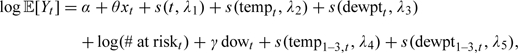where Y_t is the number of admissions for cardiovascular disease and x_t is the county-wide average of the chemical component being examined. When we use the regression calibration approach, x_t is estimated using the regression calibration function $𝔼[x_t|{\mathbf{w}}_t]$, and with the 2-stage Bayesian model, the values of x_t are sampled from the full conditional distribution within the MCMC iterations. We assume that the variables other than the pollutant variable are measured without error.

The additional terms in the model represent an offset for the number of people at risk, the day of the week, a smooth function of the 3-day running mean of temperature, and a smooth function of the 3-day running mean of dew point temperature. The running means of temperature are included to capture the effects of temperature in the winter (Samet and others, 1998). For the smooth functions, we used ${\lambda }_1=49$, ${\lambda }_2={\lambda }_4=6$, and ${\lambda }_3={\lambda }_5=3$. These values have been used previously and generally capture the variation in season as well as temperature (Peng and others, 2006; Welty and Zeger, 2005).

Estimates of the risk parameter θ are shown in Table 5. The results are shown for estimates obtained using standard maximum likelihood, which ignores the spatial misalignment problem, as well as regression calibration and the 2-stage Bayesian model which explicitly adjust for spatial misalignment error. For the Bayesian model, we use the posterior mean as our point estimate and the posterior standard deviation as our measure of uncertainty. Table 5 shows the 5 largest counties (by population) of the 20 counties we examined.

Table 5.

Estimates and standard errors (in parentheses) of the percent increase in cardiovascular hospital admissions associated with a 1 interquartile range (IQR) increase in the chemical component using standard maximum likelihood (MLE), regression calibration (RegCal), and the 2-stage Bayesian model (Bayes). The values shown are . For the 2-stage Bayesian model, is the posterior mean. The IQRs for each component are expressed in μg/m³ and are 3.06 (sulfate), 1.64 (nitrate), 0.07 (silicon), 0.40 (EC), 3.18 (OCM), 0.11 (sodium ion), and 1.35 (ammonium)

US county	Method	Estimates (standard errors)
		Sulfate	Nitrate	Silicon	EC	OCM	Sodium Ion	Ammonium
Los Angeles, CA	MLE	0.66(1.10)	0.10(0.24)	− 0.38(0.59)	1.25(0.61)	− 0.65(0.88)	0.34(0.41)	0.17(0.44)
	RegCal	1.29(2.17)	− 0.02(0.42)	− 0.47(1.15)	3.74(2.02)	− 2.90(1.73)	4.01(2.35)	− 0.02(0.80)
	Bayes	1.30(2.22)	0.00(0.41)	0.81(1.56)	4.02(1.99)	− 2.64(1.61)	4.93(1.64)	− 0.04(0.82)
Cook, IL	MLE	− 0.79(0.65)	− 0.16(0.42)	0.31(0.30)	− 0.06(0.56)	− 0.79(0.87)	2.05(0.93)	− 0.55(0.55)
	RegCal	− 0.78(0.77)	0.32(0.52)	0.50(0.46)	0.25(1.24)	− 0.05(1.29)	5.85(3.09)	− 0.26(0.68)
	Bayes	− 0.80(0.76)	0.30(0.52)	0.63(0.49)	0.02(1.33)	− 0.27(1.32)	4.13(0.98)	− 0.27(0.68)
Maricopa, AZ	MLE	− 0.49(6.93)	0.65(1.42)	0.18(0.28)	0.66(0.71)	0.02(1.10)	− 1.74(1.00)	3.79(3.46)
	RegCal	9.80(10.67)	2.76(2.72)	0.46(0.82)	3.21(2.73)	1.28(2.68)	− 1.40(5.56)	6.91(4.83)
	Bayes	8.96(11.03)	1.78(2.89)	0.40(0.86)	2.89(2.85)	1.00(2.75)	1.36(4.30)	6.49(5.16)
San Diego, CA	MLE	− 0.16(2.39)	0.67(0.67)	1.15(0.90)	2.00(1.24)	3.02(1.27)	0.05(0.41)	0.10(1.15)
	RegCal	0.58(3.58)	0.50(0.76)	1.05(1.15)	4.13(2.51)	2.46(2.11)	− 1.30(2.80)	− 0.06(1.33)
	Bayes	− 0.38(3.76)	0.64(0.78)	1.46(1.12)	5.97(2.70)	3.03(2.21)	− 2.02(2.73)	− 0.26(1.38)
Queens, NY	MLE	2.31(1.03)	0.64(0.96)	0.96(0.87)	0.53(0.78)	0.17(0.96)	0.10(0.06)	1.44(0.88)
	RegCal	2.47(1.11)	0.90(1.00)	0.84(1.37)	2.15(1.28)	0.80(1.19)	1.24(0.68)	1.82(0.98)
	Bayes	2.68(1.15)	0.82(1.04)	1.04(1.55)	1.35(1.43)	0.63(1.22)	1.27(0.68)	1.90(1.04)

The point estimates from the regression calibration procedure and the 2-stage Bayesian model are generally in agreement given the uncertainties. The standard errors for the Bayesian estimates tend to be slightly larger than the standard errors obtained using the regression calibration procedure. We see in Table 5 that the chemical components that exhibited greater spatial misalignment error resulted in larger adjustment for their estimated risk parameters. However, for components where there did not appear to be a strong association to begin with (e.g. silicon), the adjusted estimates from the regression calibration and Bayesian models were not substantially different from the maximum likelihood estimates. In the supplementary material, we show the point risk estimates for each component in all 20 counties (Figures 7–13, available at Biostatistics online).

Figure 14 of the supplementary material (available at Biostatistics online) shows the inverse-variance weighted average of the risk estimates across all 20 counties for each component and each model. EC and sodium ion are relatively heterogeneous spatially, and we see that across the 20 counties the adjustment for spatial misalignment changes the point estimates substantially. Sulfate and ammonium are much more spatially homogeneous, and we can see from Figure 14 of the supplementary material (available at Biostatistics online) that the adjustment for spatial misalignment has little effect here. The other components showed only modest differences in their point estimates between the 3 models.

6. DISCUSSION

We have presented a statistical model for estimating short-term health risks of air pollution from time series studies while adjusting for spatial misalignment error. We demonstrated a regression calibration approach that is computationally very efficient as well as a 2-stage Bayesian model. These approaches were used to estimate the risk of cardiovascular hospitalization associated with exposure to chemical components of PM.

The methods proposed in this paper will likely be useful when (1) one wishes to estimate the risk of ambient exposure to a very spatially heterogeneous pollutant such as EC and (2) there are few monitors available inside a county, but monitors exist outside the county so that information about spatial variability of a pollutant can be “borrowed” from outside the county by fitting a spatial–temporal model to all available data.

Our findings indicate that the effect of spatial misalignment depends on monitor coverage within a county and the spatial variability of the pollutant of interest. In general, a decrease in the area covered per monitor in a county is associated with lower spatial misalignment error, and this effect is far more pronounced for pollutants that are inherently heterogeneous such as sodium ion, silicon, and EC. In particular, for counties with only one monitor, it would seem that there may be some benefit to using one additional monitor in the county. Results of our data analysis show that the largest differences in the risks estimated by our methods are observed in areas where there is a large ratio of the county area to the number of monitors.

In our application, we found that health risk estimates for EC, a pollutant exhibiting large spatial heterogeneity, were generally larger using approaches that accounted for spatial misalignment. The adjusted estimates exhibited the classic bias–variance trade-off with their substantially inflated standard errors. This increased statistical uncertainty comes from accounting for the lack of information about levels of the pollutant at all points in the county. For homogeneous pollutants (e.g. sulfate, ammonium), the information available from the monitoring network provides sufficient information about county-wide levels so that adjusted risk estimates are largely unchanged. In general, the pattern of effects observed for the chemical components of PM in this analysis is consistent with our previous population health studies incorporating the STN data (Bell and others, 2009; Peng and others, 2009).

Both the regression calibration approach and the 2-stage Bayesian model produced similar adjusted risk estimates in the 20 counties analyzed. However, in general, regression calibration should be used with care in generalized linear models with nonlinear link functions because a separate bias can be introduced in those situations (Carroll and others, 2006). Although we employed log-linear models in this application, the small size of the regression coefficients likely produced a nearly linear model, potentially explaining the similar estimates given by the 2 approaches.

There exist several alternative approaches to estimate exposures for locations without monitors and also for temporal periods without measurement for use in health-based air pollution research. These include inverse distance weighting incorporating population density (Ivy and others, 2008), air quality modeling (Bell, 2006), and kriging (Leem and others, 2006). However, some of these approaches are computational intensive and rely on data sets beyond those typically used in epidemiological settings. Our approach has the advantage of relying exclusively on existing data sets that are commonly used in air pollution studies, and our results can provide insight into the interpretation of results based on simple county average exposure metrics, such as results across different components or areas with different monitor coverage.

We must be cautious in translating our results into specific recommendations for monitor placement. Our analysis did not take into account the placement of the monitors in the county and the density of the population. For counties with very high population density concentrated in one specific area, a single monitor might be sufficient and it would make little sense to place monitors throughout the county where few people live. Further research is certainly needed in order to determine the optimal usage and placement of pollution monitors. The design of monitoring networks is generally important for regulatory purposes and cost trade-offs may be prohibitive as well. Our methodology could be extended to provide a quantitative basis for assessing the placement of monitors.

There are a number of limitations to our approach that deserve some comment. First, our use of the Gaussian process in our spatial–temporal model was a convenient simplification and may require modification depending on the nature of the data. In particular, a log-Gaussian model may be more appropriate if the data are skewed. Also related to the spatial–temporal modeling is the assumption of isotropy and separability of time and space. Given the sparsity of the monitoring network, we are skeptical of our ability to fit more complex models. Nevertheless, we admit that this is an aspect of our work in need of further investigation. The small values of κ along with the large values of the ϕ estimated in the Matérn model suggest that the model may be trying to compensate for misspecification of the correlation structure. In particular, there could be a number of factors that produce sharp changes in the pollutant surface that cannot be adequately modeled with a constant scale parameter ϕ. A logical path to explore in this context would be the use of nonstationary correlation models that can adapt to unknown heterogeneity in the underlying process (Paciorek and Schervish, 2006). Perhaps, another symptom of the lack of fit of the spatial–temporal model is the moderate correlation observed between the errors assumed by the classical error model and the estimated county-wide ambient average (Section 5.1). While the classical error assumption is not needed for the health risk estimation, it was used to estimate τ², the spatial misalignment error variance.

Another limitation of our methodology is that the spatial–temporal model is estimated and then considered fixed in the health risk estimation. As a result, uncertainty about the parameters in the spatial–temporal model is not propagated through the risk model leading to a potential underestimation of uncertainty in the risk parameters. We note, however, that there is a substantial amount of data for estimating the parameters in the spatial–temporal model and that they appear to have been estimated to reasonable precision. In addition, our approach has the advantage that it greatly simplifies the analysis of multiple health outcomes by removing the need to refit the spatial–temporal model separately for every health outcome examined.

One extension to our model would be to incorporate population density information, if available. In our spatial–temporal pollutant process, we create the county-wide averages by integrating the process against a uniform density over the county boundary. However, if we could specify a function $g\left(\mathbf{s}\right)$ which indicates the proportion of population at location s, then we could compute the following county-wide average instead:

This value x_t might reflect more accurately the population-level exposure than our current approach. We consider this an interesting avenue for future work. It should be noted, however, that this approach is subject to a different type of error, namely exposure misclassification, if residents of a county/region do not spend the majority of their time in the area where they live.

A second natural extension of our model would be to extend it to the multisite setting where data are available for many locations. Our approach here was to apply the single-location model described in Section 3 independently to each available county. However, a unified model for multiple locations would estimate location-specific and national average risks while borrowing strength across locations. Developing a multi-pollutant version of this model which incorporates correlations between pollutants would be a third extension (e.g. Shaddick and Wakefield, 2002). This extension is potentially important because in a multi-pollutant model, pollutants that are measured with error could bias risk estimates for pollutants that are measured without error. Finally, employing a spatial–temporal model for pollutants could be useful in cross-sectional studies of chemical components of PM_2.5. In particular, the model could be integrated across time to obtain a long-term average concentration which could be compared with long-term mortality rates across locations.

Ultimately, the best way to address the problem of spatial misalignment might be to move away from the county-based summaries of the outcome of interest when possible and begin using summaries with finer spatial resolution, such as zip codes. Unfortunately, many types of health data are simply not available at finer spatial resolution, and we often must accept what is available. Furthermore, due to activity patterns, a high spatial resolution does not necessarily better capture personal exposure than a larger area when individuals move between areas (e.g. live in one zip code, but work in another). Thus, there is a strong need for methods that address spatial misalignment of air pollutant concentrations used in health studies. In such cases, the methods proposed here should be useful for determining the magnitude of the errors incurred and for obtaining adjusted risk estimates.

SUPPLEMENTARY MATERIAL

Supplementary material is available at http://biostatistics.oxfordjournals.org.

FUNDING

United States Environmental Protection Agency through a STAR grant to the Johns Hopkins University (RD832417); National Institute for Environmental Health Sciences (ES012054-03 to R.P. and R01ES015028 to M.B.); National Institute for Environmental Health Sciences Center in Urban Environmental Health (P30ES03819 to R.P.).

APPENDIX A

A.1. Algorithm for fitting the 2-stage Bayesian model

We propose the following Metropolis–Hastings sampling algorithm for sampling from the joint posterior density of θ and x, where x represents the vector of unobserved true county-wide daily average chemical component levels and w is the vector of observed daily monitor average values. Briefly, the full conditionals for both θ and x are sampled using a Metropolis–Hastings rejection step. All calculations were done using R version 2.7.1 (R Development Core Team, 2008).

We make use of the profile likelihood for θ and x which profiles out the many nuisance parameters in the likelihood (Cheng and Kosorok, 2008). These parameters include the spline coefficients for the smooth function of time and the nonlinear functions of temperature and dew point temperature. Including these parameters in the model would complicate implementation and make prior specification difficult. The use of the profile likelihood simplifies the MCMC algorithm, but it comes at a cost of theoretical unity given that the profile likelihood is not a proper likelihood. However, we note that the results of the 2-stage Bayesian model closely mirror the results of the regression calibration method.

Let η be the vector of nuisance parameters in the full likelihood. We evaluate the profile likelihood $L_{\text{p}}(\theta ,\mathbf{x})={max}_{\mathbf{\eta }}{L}_f(\theta ,\mathbf{x},\mathbf{\eta })$, where for each pair of values $(\theta ,\mathbf{x})$, we maximize the full Poisson likelihood $L_{\text{f}}$ with respect to η. This can be done simply by fitting a standard generalized linear model with an offset for θ and x. Then in the steps to sample θ and x, we use the profile likelihood to calculate the acceptance ratios.

1. Sampling θ. We use a random walk Metropolis step so that the proposal distribution at step i is

   

   where is the variance of the maximum likelihood estimate of θ. The acceptance ratio is then calculated as

   

   where the prior $\pi \left(\theta \right)$ is taken to be a Normal distribution with mean 0 and standard deviation 10.
2. Sampling x. We sample the vector x as a block of length T, where T is the number of observations we have for a given county. The prior distribution for x is the posterior distribution specified in (3.6) and derived from fitting the spatial model described in Section 3. For the proposal distribution, we use the distribution in (3.6) so that the proposal equals the prior. Given a proposal value x^☆, we compute the acceptance ratio, which in this case is simply the profile likelihood ratio,

   

Each sampler was run for 10 000 iterations. Convergence of the chains was diagnosed by estimating Monte Carlo standard errors of the parameters using the method of batch means described in Jones and others (2006).

References

- Banerjee S, Carlin BP, Gelfand AE. Hierarchical Modeling and Analysis for Spatial Data. Boca Raton, FL: Chapman and Hall/CRC; 2004. [Google Scholar]
- Bell ML. The use of ambient air quality modeling to estimate individual and population exposure for human health research: a case study of ozone in the Northern Georgia region of the United States. Environment International. 2006;32:586–593. doi: 10.1016/j.envint.2006.01.005. [DOI] [PubMed] [Google Scholar]
- Bell ML, Dominici F, Ebisu K, Zeger SL, Samet JM. Spatial and temporal variation in PM2.5 chemical composition in the United States for health effects studies. Environmental Health Perspectives. 2007;115:989–995. doi: 10.1289/ehp.9621. [DOI] [PMC free article] [PubMed] [Google Scholar]
- Bell ML, Ebisu K, Peng RD, Samet JM, Dominici F. Hospital admissions and chemical composition of fine particle air pollution. American Journal of Respiratory and Critical Care Medicine. 2009;179:1115–1120. doi: 10.1164/rccm.200808-1240OC. [DOI] [PMC free article] [PubMed] [Google Scholar]
- Carroll RJ, Ruppert D, Stefanski L, Crainiceanu CM. Measurement Error in Nonlinear Models: A Modern Perspective. Boca Raton, FL: Chapman and Hall/CRC; 2006. [Google Scholar]
- Cheng G, Kosorok MR. The penalized profile sampler. Journal of Multivariate Analysis. 2008;100:345–362. doi: 10.1016/j.jmva.2008.05.001. [DOI] [PMC free article] [PubMed] [Google Scholar]
- Dominici F, Peng RD, Bell ML, Pham L, McDermott A, Zeger SL, Samet JM. Fine particulate air pollution and hospital admission for cardiovascular and respiratory diseases. Journal of the American Medical Association. 2006;295:1127–1134. doi: 10.1001/jama.295.10.1127. [DOI] [PMC free article] [PubMed] [Google Scholar]
- Dominici F, Zeger SL, Samet JM. A measurement error model for time-series studies of air pollution and mortality. Biostatistics. 2000;2:157–175. doi: 10.1093/biostatistics/1.2.157. [DOI] [PubMed] [Google Scholar]
- Fuentes M, Song H-R, Ghosh SK, Holland DM, Davis JM. Spatial association between speciated fine particles and mortality. Biometrics. 2006;62:855–863. doi: 10.1111/j.1541-0420.2006.00526.x. [DOI] [PubMed] [Google Scholar]
- Gryparis A, Paciorek CJ, Zeka A, Schwartz J, Coull BA. Measurement error caused by spatial misalignment in environmental epidemiology. Biostatistics. 2008;10:258–274. doi: 10.1093/biostatistics/kxn033. [DOI] [PMC free article] [PubMed] [Google Scholar]
- Ivy D, Mulholland JA, Russell AG. Development of ambient air quality population-weighted metrics for use in time-series health studies. Journal of Air and Waste Management Association. 2008;58:711–720. doi: 10.3155/1047-3289.58.5.711. [DOI] [PMC free article] [PubMed] [Google Scholar]
- Jones GL, Haran M, Caffo BS, Neath R. Fixed-width output analysis for Markov chain Monte Carlo. Journal of the American Statistical Association. 2006;101:1537–1547. [Google Scholar]
- Katsouyanni K, Toulomi G, Samoli E, Gryparis A, LeTertre A, Monopolis Y, Rossi G, Zmirou D, Ballester F, Boumghar A and others. Confounding and effect modification in the short-term effects of ambient particles on total mortality: results from 29 European cities within the APHEA2 project. Epidemiology. 2001;12:521–531. doi: 10.1097/00001648-200109000-00011. [DOI] [PubMed] [Google Scholar]
- Leem JH, Kaplan BM, Shim YK, Pohl HR, Gotway CA, Bullard SM, Rogers JF, Smith MM, Tylenda CA. Exposures to air pollutants during pregnancy and preterm delivery. Environmental Health Perspectives. 2006;114:905–910. doi: 10.1289/ehp.8733. [DOI] [PMC free article] [PubMed] [Google Scholar]
- Nocedal J, Wright SJ. Numerical Optimization. New York: Springer; 1999. [Google Scholar]
- Paciorek CJ, Schervish MJ. Spatial modelling using a new class of nonstationary covariance functions. Environmetrics. 2006;17:483–506. doi: 10.1002/env.785. [DOI] [PMC free article] [PubMed] [Google Scholar]
- Peng RD, Bell ML, Geyh AS, McDermott A, Zeger SL, Samet JM, Dominici F. Emergency admissions for cardiovascular and respiratory diseases and the chemical composition of fine particle air pollution. Environmental Health Perspectives. 2009;117:957–963. doi: 10.1289/ehp.0800185. [DOI] [PMC free article] [PubMed] [Google Scholar]
- Peng RD, Chang HH, Bell ML, McDermott A, Zeger SL, Samet JM, Dominici F. Coarse particulate matter air pollution and hospital admissions for cardiovascular and respiratory diseases among Medicare patients. Journal of the American Medical Association. 2008;299:2172–2179. doi: 10.1001/jama.299.18.2172. [DOI] [PMC free article] [PubMed] [Google Scholar]
- Peng RD, Dominici F, Louis TA. Model choice in time series studies of air pollution and mortality (with discussion) Journal of the Royal Statistical Society, Series A. 2006;169:179–203. [Google Scholar]
- R Development Core Team. R: A Language and Environment for Statistical Computing. Vienna, Austria: R Foundation for Statistical Computing; 2008. [Google Scholar]
- Ribeiro PJ, Diggle PJ. geoR: a package for geostatistical analysis. R News. 2001;1:14–18. [Google Scholar]
- Samet JM, Dominici F, Zeger SL, Schwartz J, Dockery DW. The National Morbidity, Mortality, and Air Pollution Study, Part I: Methods and Methodological Issues. Cambridge, MA: Health Effects Institute; 2000. [PubMed] [Google Scholar]
- Samet JM, Zeger SL, Dominici F, Curriero F, Coursac I, Dockery DW, Schwartz J, Zanobetti A. The National Morbidity, Mortality, and Air Pollution Study, Part II: Morbidity and Mortality from Air Pollution in the United States. Cambridge, MA: Health Effects Institute; 2000. [PubMed] [Google Scholar]
- Samet JM, Zeger SL, Kelsall J, Xu J, Kalkstein L. Does weather confound or modify the association of particulate air pollution with mortality? Environmental Research, Section A. 1998;77:9–19. doi: 10.1006/enrs.1997.3821. [DOI] [PubMed] [Google Scholar]
- Shaddick G, Wakefield J. Modelling daily multivariate pollutant data at multiple sites. Applied Statistics. 2002;51:351–372. [Google Scholar]
- Touloumi G, Atkinson R, Le Tertre A, Samoli E, Schwartz J, Schindler C, Vonk J, Rossi G, Saez M, Rabszenko D and others. Analysis of health outcome time series data in epidemiological studies. Environmetrics. 2004;15:101–117. [Google Scholar]
- Welty LJ, Zeger SL. Are the acute effects of PM10 on mortality in NMMAPS the result of inadequate control for weather and season? A sensitivity analysis using flexible distributed lag models. American Journal of Epidemiology. 2005;162:80–88. doi: 10.1093/aje/kwi157. [DOI] [PubMed] [Google Scholar]
- Zeger SL, Thomas D, Dominici F, Samet JM, Schwartz J, Dockery D, Cohen A. Exposure measurement error in time-series studies of air pollution: concepts and consequences. Environmental Health Perspectives. 2000;108:419–426. doi: 10.1289/ehp.00108419. [DOI] [PMC free article] [PubMed] [Google Scholar]
Associated Data
This section collects any data citations, data availability statements, or supplementary materials included in this article.