Genome-wide association of breast cancer: composite likelihood with imputed genotypes

Abstract

We describe composite likelihood-based analysis of a genome-wide breast cancer case–control sample from the Cancer Genetic Markers of Susceptibility project. We determine 14 380 genome regions of fixed size on a linkage disequilibrium (LD) map, which delimit comparable levels of LD. Although the numbers of single-nucleotide polymorphisms (SNPs) are highly variable, each region contains an average of ∼35 SNPs and an average of ∼69 after imputation of missing genotypes. Composite likelihood association mapping yields a single P-value for each region, established by a permutation test, along with a maximum likelihood disease location, SE and information weight. For single SNP analysis, the nominal P-value for the most significant SNP (msSNP) requires substantial correction given the number of SNPs in the region. Therefore, imputing genotypes may not always be advantageous for the msSNP test, in contrast to composite likelihood. For the region containing FGFR2 (a known breast cancer gene) the largest χ² is obtained under composite likelihood with imputed genotypes (χ₂² increases from 20.6 to 22.7), and compares with a single SNP-based χ₂² of 19.9 after correction. Imputation of additional genotypes in this region reduces the size of the 95% confidence interval for location of the disease gene by ∼40%. Among the highest ranked regions, SNPs in the NTSR1 gene would be worthy of examination in additional samples. Meta-analysis, which combines weighted evidence from composite likelihood in different samples, and refines putative disease locations, is facilitated through defining fixed regions on an underlying LD map.

Introduction

Genome-wide association mapping studies based on large case–control samples^{1, 2} have identified common genetic variants associated with increased risk of breast cancer. Most analyses of genome-wide case–control data sets employ tests based on individual single-nucleotide polymorphisms (SNPs).³ Meta-analysis (combining evidence across samples) is facilitated by imputation of ‘missing' SNP genotypes, using the HapMap samples (http://www.hapmap.org/) as a reference population.⁴ An alternative approach to single SNP tests^{5, 6} undertakes composite likelihood analysis of multiple SNPs in a region and determines a location for a putative disease influencing variant on an underlying linkage disequilibrium unit (LDU) map.⁷ When plotted against physical (kb) locations the LDU map describes the underlying pattern of linkage disequilibrium (LD) as a series of plateaus (strong LD) and steps (where LD is breaking down, such as at the location of recombination hot spots). The LDU map provides a framework for characterising small chromosome regions, which may differ substantially in physical size but share comparable levels of LD. Modelling the pattern of association with disease at multiple markers in a region generates a single P-value for disease association, a disease location, SE and corresponding information weight. As there is just one statistical test in a region, there is a reduced Bonferroni correction relative to single SNP-based tests, which require consideration of the number of tests made at nearby SNPs. Gibson et al⁵ evaluated the composite likelihood approach using relatively low-density genotype data (∼200K SNPs) in a relatively small sample (403 cases and 395 controls) with an undisclosed disease phenotype. Larger and more comprehensively genotyped samples are now available. The genome-wide breast cancer association analysis by Hunter et al² utilised samples from 1145 postmenopausal women of European ancestry with invasive breast cancer contrasted with 1142 controls analysed with 528 173 SNPs. These data are made available through the Cancer Genetic Markers of Susceptibility (CGEMS) project data portal (http://cgems.cancer.gov/). The data are valuable for comparing composite likelihood and single-marker analyses and for developing strategies for meta-analysis. These data present significant evidence for a now well-established breast cancer gene, FGFR2, which has been verified in several studies.¹ We describe the application of a composite likelihood modelling approach to this higher-density SNP sample, evaluate relative power for composite likelihood and single SNP-based tests and test the impact of increasing marker coverage through genotype imputation. The chromosome region-based approach used in composite likelihood, with regions defined on the underlying LDU map, is highly suited to meta-analysis, which is essential to increase the sample size for the identification of novel causal variants.

Materials and methods

Data preparation and quality control

Following successful application for permissions, data comprising 1145 cases and 1142 controls and genotypes for 555 148 SNPs were downloaded from the CGEMS data portal. Data files were converted into PLINK format⁸ and quality control (QC) procedures undertaken. Samples rejected through the QC employed by Hunter et al² had already been excluded in the downloaded data set from an original set of 1183 cases and 1185 controls. The QC we applied resulted in the removal of 93 SNPs with inconsistent or ambiguous kilobase locations, 8648 SNPs with a high proportion (>10%) missing genotypes, 53 615 SNPs with minor allele frequencies lower than 0.05 and a further 4308 SNPs with large deviations from Hardy–Weinberg (χ² ≥10) in the controls (Supplementary Table 1). In addition, one individual with >10% missing genotypes was excluded at the QC stage. To minimise biases created by population stratification, we identified individuals with possible non-Caucasian ancestry through multidimensional scaling cluster analysis⁸ (Supplementary Figures 1 and 2) using 73 560 ‘LD-independent' SNPs from CGEMs and HapMap. A total of 12 907 of these SNPs showed strand mismatches and were flipped accordingly. No A/T or G/C SNPs were genotyped in the CGEMS data because of the chemistry of the genotyping beadchip (Infinium II; Illumina, Inc., San Diego, CA, USA). This cluster analysis identified four individuals who were judged to be outside the CEU cluster, suggesting admixture, and were excluded from further analysis at this point. Following QC, we analysed a total of 498 786 SNPs in 1143 cases and 1139 controls.

Genotype imputation

After flipping strands for 94 489 SNPs, to ensure strand concordance of the two SNP data sets, a combined CGEMS and HapMap (CEU, phase 3) data set was produced for genome-wide genotype imputation using the PLINK software. Accepting the suggested thresholds for ‘sufficiently imputed' markers (http://pngu.mgh.harvard.edu/~purcell/plink/haplo.shtml), (INFO values >0.8 and imputation rate across the combined sample ≥0.9), we retained 544 683 imputed SNPs (∼34% of all imputed genotypes). Further QCs applied to the aggregated data set identified 308 imputed SNPs with >10% missing genotypes, 49 019 SNPs with minor allele frequencies <0.05 and 6800 SNPs deviating significantly from Hardy–Weinberg in the controls. These 56 127 QC-failed SNPs were removed leaving a total of 488 991 imputed SNPs to be analysed in combination with the original genotypic data (Supplementary Figure 3).

Composite likelihood tests

The program CHROMSCAN⁹ develops the model described by Maniatis et al¹⁰ utilising data from SNPs in a chromosome region to compute a maximum likelihood location, S, for a causal variant, SE, a 95% confidence interval and a permutation-based P-value. The underlying LD structure is incorporated into the model through LDU maps, which represent the association mapping analogue of the linkage map.¹¹ Disease mapping on the underlying LDU scale has been shown to increase fine mapping resolution and power relative to the physical (kilobase) map.⁹ We constructed LDU maps from the CEU sample from HapMap Phase II based on physical locations from build 36 of the human genome sequence (University of California, Santa Clara, March 2006). Genome-wide LDU maps¹² are available on request from the authors.

The association test reduces the 3 × 2 table of SNP genotype counts by disease affection status at the i^th SNP to the corresponding 2 × 2 table of allele counts by affection status, with cell totals a, b, c, d, giving n haplotypes from n/2 diplotypes. Association of disease phenotype with SNPs in a region is modelled using a composite likelihood approach. Observed association with disease at the i^th SNP is: with information Expected association, z_i, is modelled using the Malecot equation:¹⁰ where S_i is the location of the i^th SNP in LDU and the S parameter represents the LDU map location showing maximal association with disease. The ɛ parameter describes the decline of association with map distance and has a value ∼1 for LDU maps,⁹ M is the intercept and L is the asymptote, representing association not due to linkage, which is estimated (L) or predicted (L_p). The predicted asymptote is taken as the mean absolute value of a standard normal deviate, weighted by information K_z.⁹ Composite likelihood is defined as: lk=e^−Λ/2, where CHROMSCAN evaluates the composite likelihood for two subhypotheses to test the evidence for a disease-associated variant in a region. Within a given region the null hypothesis (‘model A') assumes only ‘background' association and no relationship between the affection status and SNPs with: L=L_p, M=0. As the null model does not test association with disease, there is no location estimate, S. The null model, which estimates no parameters, is contrasted with ‘model D', which estimates three parameters: a disease location (S), an intercept (M) and background association (L).

The association test statistic for each region is the difference X=Λ_A−Λ_D. The difference is computed for the real data (H₁) and a large number of replicates (H₀), as X_j for the j^th replicate, in which the disease phenotype is randomised (shuffled). The distribution of P-values under H₀ is obtained from fractional ranks in a large sample of replicates. From each of the replicate, P-values the corresponding χ₃² for the contrast between models ‘A' and ‘D' is obtained from the GNU Scientific Library (GSL) function gsl_cdf_chisq_Pinv (http://www.gnu.org/software/gsl/), and hence the variance for the j^th replicate is: 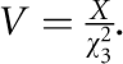Variances for replicates, V_j, are used to predict, by regression, variance V (H₁) and hence χ₃² (H₁). The computation of V (H₁) requires a sorted subset of replicates, which are centred on the value X (H₁), and the model: lnV_j=A+B lnX_j, with X centred between the 20 closest replicates with X_j≤X and the corresponding 20 with X_j≥X; if X is an outlier, the 20 closest values are taken. From this model V (H₁) is estimated as exp(A+BlnX), and χ₃²(H₁)=X/V.

Simultaneous estimates of M, S and L give an information matrix, which is inverted to provide the nominal variance (U) for location S. Using V (H₁), the information weight, W, about disease gene location, S, is computed as: 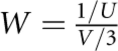and the SE of S is: We revised CHROMSCAN to increment the number of replicates adaptively to ensure that the P-value (H₁) predicted from the replicates is accurately determined, with a minimum of 50 replicates and maximum of 20 000 per region (or more for refining evidence in a significant region of interest). Gibson et al,⁵ in their analysis of a relatively low-density SNP data, used non-overlapping regions spanning at least 10 LDUs and containing a minimum of 30 SNPs. More recent high-density panels enable analysis in smaller regions and higher resolution with reduced possibility of confounding adjacent independent signals. We used regions of fixed LDU size, which facilitates combination of evidence in meta-analysis. Regions of four LDUs contain an average of over 30 SNPs in a ∼550 000 SNP scan, assuming ∼60 000 LDUs in the CEU genome.¹² However, there is wide variation in the number of SNPs per region, although coverage is increased with genotype imputation (Table 1).

Table 1. The distribution of SNPs within four-LDU regions.

SNP range	N	T	R
1–5	1120	2.22	1.67
6–10	1285	7.13	4.58
11–14	1243	11.57	6.98
15–18	1449	15.52	9.28
19–22	1595	19.52	10.46
23–25	1223	23.01	12.32
26–28	1284	25.97	14.13
29–32	1735	29.50	15.83
33–36	1647	33.50	17.24
37–39	1171	36.96	16.88
40–43	1433	40.49	18.74
44–48	1723	44.96	20.10
49–53	1496	49.98	23.68
54–59	1442	55.45	20.91
60–66	1436	61.86	24.56
67–75	1526	69.81	25.51
76–87	1536	80.19	28.04
88–104	1391	94.40	27.52
105–136	1527	117.71	30.70
137–250	1348	171.24	37.33
251–550	135	300.16	55.64
551–800	5	656.80	97.20
Total	28 750	—	—

Abbreviations: N, total number of four-LDU regions containing the number of SNPs in range; R, mean effective number of SNPs in the range (Bonferroni correction); T, weighted mean number of SNPs in the range.

Table contains regions from original and imputation data sets combined.

Single SNP tests

For single SNP tests, we identify the most significant SNP (msSNP) in a region, from the nominal χ₁² (from the 2 × 2 table between affection and the two SNP alleles). Selecting the msSNP from a large number of SNPs in a region biases the nominal P-value (P_n), computed on the null hypothesis. To correct for the number of SNPs, we first grouped four-LDU regions into ranges, which show relatively limited diversity in the number of SNPs they contain (Table 1). The ranges (SNP range, Table 1) were defined to include approximately similar numbers of four-LDU regions, with the exception of regions containing >250 SNPs. This enabled the relationship between T (the observed mean number of SNPs in the range) and R (the effective mean number of SNPs in the range) to be characterised in the tail of the distribution. We determined the distribution of numbers of SNPs in each of 28 750 four-LDU regions (original and imputation-inclusive data sets combined) and computed the weighted mean number of SNPs, T, in a range (for each range 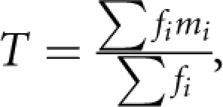where f is the number of four-LDU regions containing m SNPs, with summation over i=1, N regions; Table 1). Under the null hypothesis P-values for random SNPs have expectation χ₂²=2lnP, with an expected variance of four and a mean of two.⁵ For each range we computed, R, the effective number of independent SNPs (Table 1) by regula falsi. Bonferroni correction assumes a corrected P-value: P_c=1−(1−P_n)^R. To correct P-values from single SNPs, we determined the relationship between R and T by regression such that a value R could be assigned to each four-LDU region, given T. Regression through the origin gives R_s=(0.306239 × T)−(0.000248 × T²), (model R²=0.96), which enables Bonferroni corrected values P_c to be computed. The Bonferroni correction greatly reduces the significance of the nominal P-values. Composite likelihood tests do not require this correction as P-values are based on a permutation test.

Following correction of msSNP P-values for the variable number of SNPs in individual four-LDU regions, the means (μ) of the corrected χ_2c² from the msSNPs (μ=2.5 and 2.2 for original and imputation data sets respectively) and the χ₂² from permutation-based P-values in composite likelihood analyses (μ=1.9 for both original and imputation inclusive data sets) were multiplied by 2/μ to correct the deviation from the expected mean of 2.

Results

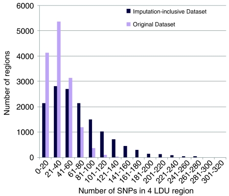
CHROMSCAN analysis yields 14 370 four-LDU regions containing at least one SNP from the original genotype data and 14 380 from the data containing imputed genotypes. The distribution of SNPs in each region is very variable (Table 1, Figure 1). Many regions contain ≤20 SNPs and, as the LDU map describes regions with comparable levels of LD, this suggests that a substantial proportion of the genome may be poorly screened by this set of genotypes. Coverage is increased by imputation of missing genotypes, with the mean number of SNPs per region increasing from 34.7 to 68.6 (Figure 1). However, following imputation ∼15% of the regions still have ≤20 SNPs and may be poorly represented by both single SNP and composite likelihood tests. SNP panels with more uniform coverage of markers on the LDU, rather than kilobase scale, would reduce the possibility of overlooking regions associated with disease. In higher SNP density panels, the magnitude of the Bonferroni correction required for single SNP analysis will be greater. In contrast, more comprehensive genotyping may increase power for composite likelihood tests because one permutation-based P-value is obtained for every region.

Figure 1.

The distribution of SNPs in each four-LDU window in the original and imputed data sets.

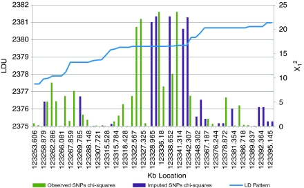
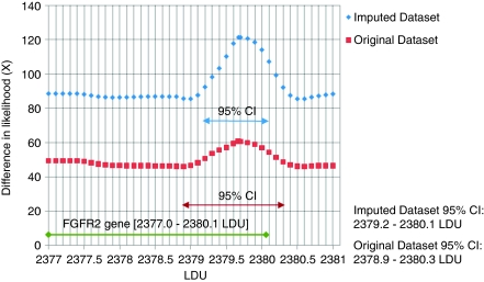
The distribution of nominal single SNPs (χ₁²) in the FGFR2 gene region (Figure 2) show a cluster of SNPs localised in a region with extensive LD represented as a plateau on the underlying LDU map. Composite likelihood mapping in this region (Table 2) indicates that, after imputation adds ∼64% more SNPs, there is an increase in χ₂² from 20.6 to 22.7. The 95% confidence interval for the location of the causal variant decreases by 40% from 1.5 to 0.9 LDUs using the more densely genotyped imputation data set. This reduction in the confidence interval, which spans intron 2 of FGFR2, is reflected in the composite likelihood surface (Figure 3), which shows the difference in X=Λ_A−Λ_D between the A (null) and D (causal variant location) models for the original and imputation inclusive data sets.

Figure 2.

Nominal single SNPs χ² for association and the LDU map of the FGFR2 region.

Table 2. Composite likelihood analysis in the FGFR2 region.

	Number of SNPs	S LDU	W	95% CI in LDU	95% CI in Kb	−2lnP
Original data set	33	2379.66 (0.36)	7.65	2378.9–2380.4 (1.5)	123311.2–123357.4 (46.2)	20.63
Imputation data set	54	2379.67 (0.24)	17.55	2379.2–2380.1 (0.9)	123315.6–123347.9 (32.3)	22.68

Abbreviations: S LDU, maximum likelihood location for disease gene (LDU), SEs in brackets; W, information weight for location S (LDU); 95% CI, 95% confidence interval for disease gene, size in brackets; −2lnP, −2 log P-value for association with disease ∼χ₂².

Figure 3.

The difference X in (composite) likelihood, where X=Λ_A−Λ_D, for null and disease association models for the original and the imputation data sets in the FGFR2 gene region.

Table 3 is ordered by the 10 most significant regions identified using composite likelihood in the imputed data set. The FGFR2 region is highest ranked for both composite likelihood and single SNP tests. Power, as indicated by −2lnP (=χ₂²), appears relatively lower in these data for single SNP tests compared with the composite likelihood-based analysis. There is quite strong correspondence between ranks in the original and imputed data sets for the five highest-ranked regions but less agreement for regions ranked 6–10. There is reduced correspondence between single SNP and composite likelihood tests, although the neurotensin receptor 1 (NTSR1) gene region has relatively high ranks for both tests.

Table 3. Composite likelihood: the ten highest-ranked regions (imputation-inclusive data set).

	Chromsomes
	10	20	2	5	20	19	15	11	1	18
Four-LDU region	2377–2381	1436–1440	1864–1868	2736–2740	1664–1668	1652–1656	1176–1180	1080–1084	812–816	516–520
Original SNPs	33	23	64	45	11	27	36	95	36	13
Imputed SNPsa	54	55	114	130	18	40	66	263	83	18
Composite −2lnP, original (rank)	20.6 (1)	16.7 (4)	18.3 (2)	14.9 (10)	17.3 (3)	11.1 (86)	14.3 (15)	12.9 (31)	15.1 (8)	12.3 (40)
Composite −2lnP, imputed (rank)a	22.7 (1)	18.8 (2)	18.5 (3)	18.1 (4)	17.5 (5)	17.3 (6)	15.4 (7)	15.4 (8)	15.4 (9)	15.3 (10)
msSNP −2lnP, original (rank)	15.9 (1)	8.8 (66)	9.6 (33)	8.7 (70)	11.2 (11)	9.2 (50)	7.3 (190)	7.8 (126)	6.3 (387)	7.8 (124)
msSNP −2lnP, imputed (rank)a	19.9 (1)	10.0 (83)	11.9 (22)	10.4 (68)	14.8 (3)	11.1 (40)	8.4 (224)	8.5 (206)	6.7 (570)	9.5 (113)
MsSNP, imputeda	rs2420946	rs2268924	rs13418293	rs9313772	rs3787521	rs381809	rs8024156	rs11600292	rs2794593	rs9956571
Geneb	FGFR2	VAPB	CNGA3	—	NTSR1	NLRP4	LOC729911	—	CSMD2	—

^a‘Imputed' herein refers to the aggregated data set consisting of both original and imputed SNPs.

^bGene including the msSNP identified.

Discussion

Comparison of composite likelihood and single SNP tests suggest higher power of the former for the FGFR2 association, which is well established as breast cancer-risk gene. Power is further increased with imputation of missing genotypes (Table 2). None of the other genes identified in Table 3 contain well-established breast cancer-risk variants, although it is notable that the NTSR1 gene ranks highly in both composite likelihood and single SNP tests. NTSR1 is a candidate risk factor involved in ductal breast cancer progression.¹³ The authors note that in breast cancer cells functionally expressed NT1 receptor coordinates transforming functions including cellular migration and invasion. High expression of NTSR1 is associated with the tumour grade, size and number of metastatic lymph nodes. Given that the well-established breast cancer genes only account for a small proportion of the familial genetic risk, regions that fail to achieve genome-wide significance, but rank highly, are worthy of examination in larger samples. A worthwhile focus of future analyses includes screening highly ranked variants in breast cancer phenotypic subtypes, including those that describe tumour characteristics.¹⁴

Hunter et al² describe the original analysis of these data and the identification of SNPs in the FGFR2 gene as highly associated with sporadic postmenopausal breast cancer. These findings were confirmed by the authors in a second sample. Although strong evidence for the involvement of FGFR2 is a feature of our analysis, comparison with the results presented by Hunter et al is difficult. Differences in the QC procedures employed (Supplementary Table 1), their use of additional phenotypic data (details of age and hormone replacement therapy use) and differences in analytical methods employed, including their use of logistic regression models, underlie the difficulty of comparison.

In the FGFR2 gene region, the apparent higher power for composite likelihood tests must be achieved partly by modelling association at multiple SNPs simultaneously. Alternative approaches that combine data from multiple SNPs include haplotype-based tests.¹⁵ Such approaches have the advantage of modelling correlations between markers, potentially increasing power, along with the characterisation of genetic effects on different haplotypic backgrounds. The disadvantages include the difficulty in deciding how to define haplotype ‘windows', the heavy computational requirements, lack of a clearly defined disease interval that is refined with accession of data and the difficulty of combining evidence across samples. Imputation of genotypes, which can usefully increase coverage and potentially provide further increases in power, must also increase the computational and multiple-testing burden for haplotype tests, which is in line with single SNP-based analyses.

Some authors have found that imputing genotypes is rather accurate,¹⁶ but note that power increases only slightly as imputation ‘results in modest gain in genetic coverage, but worsens the multiple testing penalties'. This penalty is likely to further erode power when using more comprehensive SNP panels and with imputation at higher densities, as might be achieved (for example) using data from the 1000 genomes project (http://www.1000genomes.org/page.php). Other authors note that the typical imputation error rates of 2–6%¹⁷ may substantially decrease power and so the utility of this technique may be questioned for single SNP-based analyses.

As individual genetic effect sizes are generally low for common variants involved in complex traits, meta-analysis combining evidence across studies, is an important strategy to increase power and identify novel targets for further follow-up.⁴ A composite likelihood-based approach, in which association evidence from different genome-wide association samples is combined across corresponding regions, provides a test in which individual samples are weighted according to their information (W, Table 2). This approach also gives an estimate of disease gene location, which becomes more precise as further evidence is combined.¹⁸ The methods presented here provide a strategy for the analysis of component samples in such a meta-analysis taking advantage of genotype imputation to increase coverage without increasing the multiple-testing penalty.

Polymorphisms in intron 2 of the FGFR2 gene have been implicated as increasing risk of breast cancer in European and Asian populations. Easton et al¹ reported two SNPs, rs2981582 and rs7895676 (at the upstream and downstream boundaries respectively of intron 2), as the most strongly associated and suggested that the latter was most likely to be a causal variant as it showed the strongest association with breast cancer risk. Recently, Boyarskikh et al,¹⁹ studying a West Siberian population, noted that rs2981582 explained association with disease much more strongly than rs7895676. The authors hypothesised that the actual causal variant lies somewhere within the LD block that includes these two SNPs. Although rs7895676 (location 123323.987 kb) is not represented in the imputation-inclusive data set, and rs2981582 does not have the highest single-marker χ² in the sample (Table 3), these markers flank the cluster of associated SNPs in the intron 2 LD block (Figure 2). Given that intron 2 lies within a strong LD block, fine mapping to confirm the location of the causal variant will be facilitated by meta-analysis in which the appropriately weighted accessions of data should enable further reduction of the target confidence interval.

The authors declare no conflict of interest.

References

- Easton DF, Pooley KA, Dunning AM, et al. Genome-wide association study identifies novel breast cancer susceptibility loci. Nature. 2007;447:1087–1093. doi: 10.1038/nature05887. [DOI] [PMC free article] [PubMed] [Google Scholar]
- Hunter DJ, Kraft P, Jacobs KB, et al. A genome-wide association study identifies alleles in FGFR2 associated with risk of sporadic postmenopausal breast cancer. Nat Genet. 2007;39:870–874. doi: 10.1038/ng2075. [DOI] [PMC free article] [PubMed] [Google Scholar]
- Wellcome Trust Case Control Consortium (WTCCC) Genome-wide association study of 14 000 cases of seven common diseases and 3000 shared controls. Nature. 2007;447:661–678. doi: 10.1038/nature05911. [DOI] [PMC free article] [PubMed] [Google Scholar]
- Zeggini E, Scott LJ, Saxena R, et al. Meta-analysis of genome-wide association data and large-scale replication identifies additional susceptibility loci for type 2 diabetes. Nat Genet. 2008;40:638–645. doi: 10.1038/ng.120. [DOI] [PMC free article] [PubMed] [Google Scholar]
- Gibson J, Tapper W, Cox D, et al. A multimetric approach to analysis of genome-wide association by single markers and composite likelihood. Proc Natl Acad Sci USA. 2008;105:2592–2597. doi: 10.1073/pnas.0711903105. [DOI] [PMC free article] [PubMed] [Google Scholar]
- Morton N, Maniatis N, Zhang W, Ennis S, Collins A. Genome scanning by composite likelihood. Am J Hum Genet. 2007;80:19–28. doi: 10.1086/510401. [DOI] [PMC free article] [PubMed] [Google Scholar]
- Maniatis N, Collins A, Xu C-F, et al. The first linkage disequilibrium (LD) maps: delineation of hot and cold blocks by diplotype analysis. Proc Natl Acad Sci USA. 2002;99:2228–2233. doi: 10.1073/pnas.042680999. [DOI] [PMC free article] [PubMed] [Google Scholar]
- Purcell S, Neale B, Todd-Brown K, et al. PLINK: a tool set for whole-genome association and population-based linkage analyses. Am J Hum Genet. 2007;81:559–575. doi: 10.1086/519795. [DOI] [PMC free article] [PubMed] [Google Scholar]
- Collins A, Lau W. CHROMSCAN: genome-wide association using a linkage disequilibrium map. J Hum Genet. 2008;53:121–126. doi: 10.1007/s10038-007-0226-2. [DOI] [PubMed] [Google Scholar]
- Maniatis N, Collins A, Gibson J, Zhang W, Tapper W, Morton NE. Positional cloning by linkage disequilibrium. Am J Hum Genet. 2004;74:846–855. doi: 10.1086/383589. [DOI] [PMC free article] [PubMed] [Google Scholar]
- Collins A, Lau W, De La Vega FM. Mapping genes for common diseases: the case for genetic (LD) maps. Hum Hered. 2004;58:2–9. doi: 10.1159/000081451. [DOI] [PubMed] [Google Scholar]
- Lau W, Kuo T-Y, Tapper W, Cox S, Collins A. Exploiting large scale computing to construct high resolution linkage disequilibrium maps of the human genome. Bioinformatics. 2007;23:517–519. doi: 10.1093/bioinformatics/btl615. [DOI] [PubMed] [Google Scholar]
- Dupouy S, Viardot-Foucault V, Alifano M, et al. The neurotensin receptor-1 pathway contributes to human ductal breast cancer progression. PLoS ONE. 2009;4:e4223. doi: 10.1371/journal.pone.0004223. [DOI] [PMC free article] [PubMed] [Google Scholar]
- Tapper W, Hammond V, Gerty S, et al. The influence of genetic variation in 30 selected genes on the clinical characteristics of early onset breast cancer. Breast Cancer Res. 2008;10:R108. doi: 10.1186/bcr2213. [DOI] [PMC free article] [PubMed] [Google Scholar]
- Huang BE, Amos CI, Lin DY. Detecting haplotype effects in genomewide association studies. Genet Epidemiol. 2007;31:803–812. doi: 10.1002/gepi.20242. [DOI] [PubMed] [Google Scholar]
- Hao K, Chudin E, McElwee J, Schadt E. Accuracy of genome-wide imputation of untyped markers and impacts on statistical power for association studies. BMC Genet. 2009;10:27. doi: 10.1186/1471-2156-10-27. [DOI] [PMC free article] [PubMed] [Google Scholar]
- Huang L, Wang C, Rosenberg NA. The relationship between imputation error and statistical power in genetic association studies in diverse populations. Am J Hum Genet. 2009;85:692–698. doi: 10.1016/j.ajhg.2009.09.017. [DOI] [PMC free article] [PubMed] [Google Scholar]
- Tapper W, Collins A, Morton N. Mapping a gene for rheumatoid arthritis on chromosome 18q21. BMC Proc. 2007;1:S18. doi: 10.1186/1753-6561-1-s1-s18. [DOI] [PMC free article] [PubMed] [Google Scholar]
- Boyarskikh UA, Zarubina NA, Biltueva JA, et al. Association of FGFR2 gene polymorphisms with the risk of breast cancer in population of West Siberia. Eur J Hum Genet. 2009;17:1688–1691. doi: 10.1038/ejhg.2009.98. [DOI] [PMC free article] [PubMed] [Google Scholar]
Associated Data
This section collects any data citations, data availability statements, or supplementary materials included in this article.