Joint two-view information for computerized detection of microcalcifications on mammograms

Abstract

We are developing new techniques to improve the accuracy of computerized microcalcification detection by using the joint two-view information on craniocaudal (CC) and mediolateral-oblique (MLO) views. After cluster candidates were detected using a single-view detection technique, candidates on CC and MLO views were paired using their radial distances from the nipple. Candidate pairs were classified with a similarity classifier that used the joint information from both views. Each cluster candidate was also characterized by its single-view features. The outputs of the similarity classifier and the single-view classifier were fused and the cluster candidate was classified as a true microcalcification cluster or a false-positive (FP) using the fused two-view information. A data set of 116 pairs of mammograms containing microcalcification clusters and 203 pairs of normal images from the University of South Florida (USF) public database was used for training the two-view detection algorithm. The trained method was tested on an independent test set of 167 pairs of mammograms, which contained 71 normal pairs and 96 pairs with microcalcification clusters collected at the University of Michigan (UM). The similarity classifier had a very low FP rate for the test set at low and medium levels of sensitivity. However, the highest mammogram-based sensitivity that could be reached by the similarity classifier was 69%. The single-view classifier had a higher FP rate compared to the similarity classifier, but it could reach a maximum mammogram-based sensitivity of 93%. The fusion method combined the scores of these two classifiers so that the number of FPs was substantially reduced at relatively low and medium sensitivities, and a relatively high maximum sensitivity was maintained. For the malignant microcalcification clusters, at a mammogram-based sensitivity of 80%, the FP rates were 0.18 and 0.35 with the two-view fusion and single-view detection methods, respectively. When the training and test sets were switched, a similar improvement was obtained, except that both the fusion and single-view detection methods had superior test performances on the USF data set than those on the UM data set. Our results indicate that correspondence of cluster candidates on two different views provides valuable additional information for distinguishing FPs from true microcalcification clusters.

I. INTRODUCTION

There is strong evidence that imaging the breast in two views—mediolateral oblique (MLO) and craniocaudal (CC) views—increases the cancer detection sensitivity while decreasing the recall rate.^1,2 The radiologist combines the information from the two views to confirm true positives (TPs) and to reduce false positives (FPs). It is expected that computerized detection could also benefit from the joint two-view information available in a screening study. Our laboratory has been developing image analysis methods to exploit the joint two-view information for FP reduction in computerized detection of masses³ and microcalcifications⁴ on mammograms.

In recent years, a number of research groups have investigated the use of two-view mammograms of the same breast in a given examination to improve computerized lesion analysis. Our group investigated the fusion of information from two mammographic views to improve the performance a CAD system for breast mass detection.^3,5,6 The distance between the nipple and computer-detected objects on the two views was used to geometrically pair the objects, which were then classified using a correspondence classifier. To establish the geometric relationship of the locations of the same object seen in two mammographic views, we used a data set of 116 two-view cases containing masses, microcalcification clusters, and large benign calcifications. The absolute value of the nipple-to-object distance (NOD) difference on the two views was found to be less than 16 mm for 83% of the lesions. Yam et al.⁷ and Kita et al.⁸ developed a method to extract three-dimensional (3D) information about breast lesions from two mammographic views. Their technique was based on a breast model to estimate the deformation of the canonical breast representation under compression from that without compression. The method was applied to 3D reconstruction of microcalcifications, as well as to the prediction of the lesion location on one view from the location on the other view. For a data set of 37 lesions, their method could predict the location in the second view within a band of pixels ±27 mm from an epipolar line.⁸ The average minimum distance from the epipolar line was 6.8 mm, while the average distance using the NOD difference was 8.6 mm. In a different publication,⁷ on a data set of 35 lesions, they reported average distances of 6.5 and 6.9 mm using the epipolar lines and the NOD difference, respectively. Chang et al.⁹ compared two methods for predicting a search region on the MLO view (or the CC view) for a lesion detected on the CC view (or the MLO view). The first method was based on the ratio of the NOD on the two views, and the second method was on a Cartesian straight-line distance. They found that the two methods had essentially similar performance in predicting the lesion location. Despite the efforts by many investigators in studying the geometric correspondence between the lesion locations on two mammographic views, to our knowledge the study by Paquerault et al.³ was the only journal publications to date that used two-view information to improve the single-view detection of masses. Sahiner et al.⁴ performed a preliminary study to investigate the use of joint two-view information to improve computerized microcalcification detection. The current study further improved the two-view fusion scheme and evaluated its performance with an independent data set.

II. METHODS

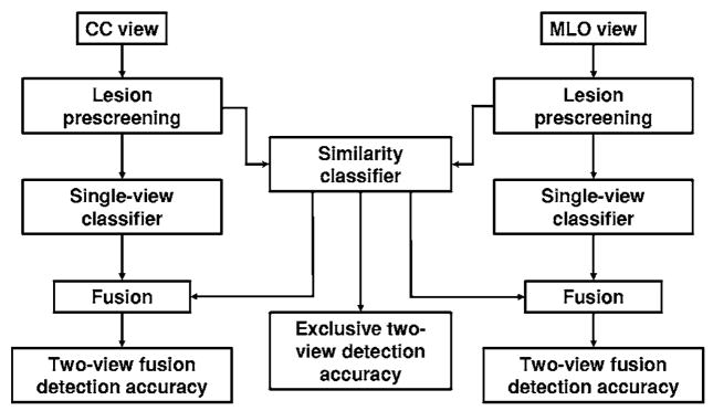
The joint two-view detection method used in this study is based on the assumption that if a single-view detection algorithm detects the corresponding true cluster on the CC and MLO views of the same breast, the TP clusters on the two views will exhibit similarities in their geometric, morphological, and textural features. A FP cluster detected on the CC view is expected to exhibit a lesser degree of similarity with the true cluster on the MLO view, and vice-versa. Similarly, the degree of similarity exhibited by two FP clusters on two different views is expected to be lesser than that between two TPs. In this study, we made use of this assumption by performing similarity analysis between cluster candidates detected on the two views and distinguishing true pairs (TP-TP pairs) from false pairs (FP-TP, TP-FP, and FP-FP pairs). We used the NOD difference to define a limited number of object pairs. The scores resulting from the similarity classifier may not provide adequate sensitivity if used alone. The reasons are twofold. First, some lesions may not be visible on both views. Second, even if a lesion is visible on both views, it may have been missed by the computer on one view. However, we found that by designing a proper strategy in which the two-view pair classification scores are fused with the single-view scores, the overall accuracy of the detection system can be significantly improved. The block diagram of the two-view fusion method is shown in Fig. 1.

Fig. 1.

The block diagram of the relationship between the single-view detection, exclusive two-view detection, and two-view detection methods. The lesion prescreening, single-view classifier, and fusion blocks for the CC and MLO views are identical.

A. Data sets

Two independent data sets collected at different institutions were used for training and testing the two-view detection algorithm. Each data set consisted of a group of two-view mammograms that contained at least one microcalcification cluster (the positive group) and a different group of two-view mammograms that were free of microcalcification clusters (the normal group).

The training data set included mammograms from the publicly available University of South Florida (USF) digitized mammogram database.¹⁰ The positive training group consisted of malignant microcalcification cases in the USF database digitized with a Lumisys 200 laser scanner (volumes: cancer_01, cancer_02, cancer_05, cancer_09, and cancer_15). This group initially contained 124 cases (124 CC and 124 MLO view mammograms). Eight cases (16 mammograms) were excluded from the positive training group because these cases contained diffuse microcalcifications scattered over a large breast area, and the correspondence of the microcalcification locations on two views cannot be established. The positive training group therefore consisted of 232 mammograms. On these positive mammograms, 254 microcalcification locations were identified, of which 235 were proven to be malignant by biopsy. The remaining 19 locations, which were detected on breasts that had undergone biopsy for a different suspicious cluster, did not have biopsy proof. The normal training group consisted of the contralateral mammograms of the patients included in the positive training group, as well as mammograms of patients with a detected breast mass in the contralateral breast. Initially, the pool of normal cases included 494 mammograms. Two MQSA radiologists at our institution examined the cases to confirm that they are free of microcalcification clusters and calcified vessels. Upon this inspection, 44 pairs of mammograms were excluded because at least one view contained a calcified vessel or a microcalcification cluster that was not marked in the USF database. Our normal training group therefore consisted of 406 mammograms (203 cases). The nipple location for each mammogram was manually identified at our institution.

The lesions in the training database were rated for their subtlety by experienced radiologists and provided with the USF database. The distribution of the subtlety ratings for the training data set is shown in Fig. 2, where 1 indicates the most obvious clusters, and 5 indicates the most subtle. Note that in order to be consistent with our rating scale in which a subtle lesion has a higher rating (e.g., Fig. 4), we reversed the original ratings in the USF database for this figure. An assessment that follows the American College of Radiology Breast Imaging Reporting and Data System (BI-RADS) categories was also provided for the clusters. The distribution of the assessment ratings for the training data set is shown in Fig. 3. Most clusters had an assessment rating of 4 (suspicious abnormality, biopsy should be considered), or 5 (highly suggestive of malignancy, appropriate action should be taken). This is consistent with the fact that all mammograms contained at least one biopsy-proven malignant microcalcification cluster.

Fig. 2.

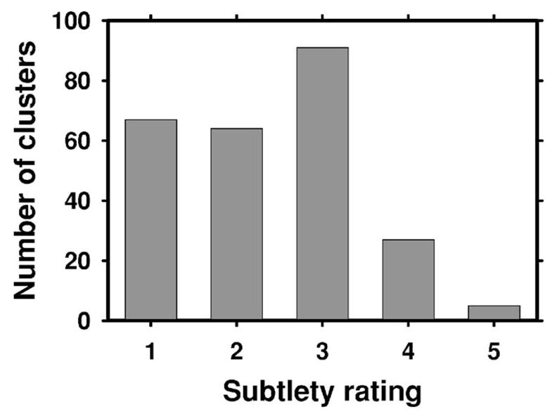
The distribution of the subtlety ratings (1: most obvious, 5: most subtle) for the microcalcification clusters in the training data set. The ratings were provided with the USF database. Note that in order to be consistent with our rating scale in which a subtle lesion has a higher rating (e.g., Fig. 4), we reversed the original ratings (and their interpretation) in the USF database for this figure.

Fig. 4.

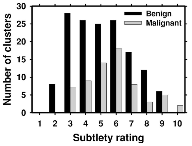
The distribution of the subtlety ratings (1: most obvious, 10: most subtle) for the malignant and benign microcalcification clusters in the test (UM) data set. The ratings were provided by MQSA radiologists at UM.

Fig. 3.

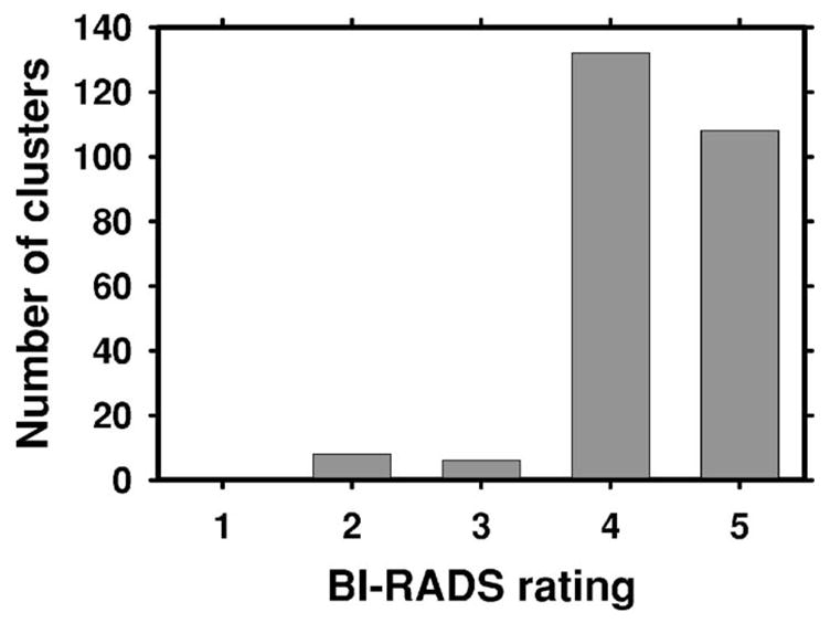
The distribution of the assessment ratings for the microcalcification clusters in the training (USF) data set. The assessment follows the American College of Radiology BI-RADS lexicon and was provided with the USF database. Since all cases had biopsy-proven malignant clusters, there were very few ratings of 2 (benign finding) and 3 (probably benign finding, short-interval follow-up suggested). A majority of the ratings were 4 (suspicious abnormality, biopsy should be considered), or 5 (highly suggestive of malignancy, appropriate action should be taken).

The test data set consisted of mammograms collected with Institutional Review Board approval at the University of Michigan (UM). The positive test group consisted of 96 pairs of mammograms, each of which contained at least one biopsy-proven microcalcification cluster. The cases were collected consecutively from our biopsy-proven mammogram database, with the exception that any case containing diffuse microcalcifications or calcified vessels was excluded. There were 218 microcalcification cluster locations marked by a MQSA radiologist on 192 mammograms. The same radiologist also established the correspondence of the clusters on two views using all the clinical information related to the case. Ten of the clusters were visible only on one mammographic view, and the remaining clusters were seen on both views. We thus had 104 clusters seen on both views, accounting for 208 marked locations. Sixty-six of the marked locations corresponded to biopsy-proven malignant clusters, and 148 locations corresponded to clusters that were benign either by biopsy or follow-up. The remaining four locations (corresponding to two clusters seen on both views) were on biopsy-proven mammograms containing malignant clusters, but their pathology could not be ascertained because these clusters did not undergo biopsy. The normal test group initially contained 100 pairs of mammograms from patients with a detected breast mass in the contralateral breast. Two MQSA radiologists examined these mammograms to confirm that they are free of microcalcification clusters and calcified vessels. The inspection revealed that 29 pairs of mammograms contained a calcified vessel or a microcalcification cluster on at least one view. Our normal test group therefore consisted of 142 mammograms (71 cases) after exclusion of the 29 pairs. The nipple location for each case was manually identified. Table I summarizes the training and test data sets.

Table I.

The positive and normal data groups for the training and test data sets.

	Training (USF data set)		Test (UM data set)
	Positive	Normal	Positive	Normal
Number of two-view cases	116	203	96	71
Number of cluster locations	254		218
Number of malignant cluster locations	235		66
Number of benign cluster			148
Number of locations with unknown status	19		4

The subtlety of the microcalcification clusters in the UM data set was rated by an experienced MQSA radiologist on a scale of 1 (obvious) to 10 (subtle) relative to the visibility range of microcalcifications encountered in clinical practice. The distribution of the subtlety ratings for benign and malignant clusters is shown in Fig. 4. It can be seen that the malignant and benign clusters had similar subtlety ratings, with the malignant clusters slightly more subtle than benign clusters. Since there are no standards or methods for calibration of the subtlety ratings across different institutions, it is not possible to compare the subtlety ratings of the UM cases with those of the USF cases. The same experienced MQSA radiologist also provided a likelihood of malignancy rating for each cluster in the UM data set. The distribution of the likelihood of malignancy ratings for benign and malignant clusters is shown in Fig. 5.

Fig. 5.

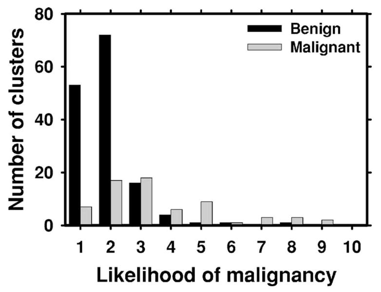
The distribution of the likelihood of malignancy ratings (1: least likely to be malignant, 10: most likely to be malignant) for the malignant and benign microcalcification clusters in the test data set. The ratings were provided by MQSA radiologists at UM.

The USF data set was digitized using a Lumisys 200 laser scanner with an optical density (OD) range of 0–3.6, and the UM data set was digitized using a LUMISCAN 85 laser scanner with an OD range of 0–4.0. Both digitizers were calibrated so that the gray values were linearly and inversely proportional to the OD, with a slope of −0.001 OD unit/pixel value. All mammograms were digitized at a pixel resolution of 0.05×0.05 mm with 4096 gray levels. The image matrix size was reduced by averaging every 2×2 adjacent pixels and down-sampling by a factor of 2, resulting in images with a pixel size of 0.1×0.1 mm for further analysis.

B. Cluster prescreening

The purpose of the lesion prescreening stage in the CAD system is to identify areas containing microcalcification cluster candidates so that these areas can be further analyzed in subsequent stages to determine whether they contain a true cluster or a FP cluster. First, the image is processed using a difference-image technique to enhance the signal-to-noise ratio (SNR) of the microcalcifications.¹¹ Second, potential signals are segmented from the image background using global and locally adaptive segmentation techniques. Rule-based classification is applied to the signal size, contrast and SNR to identify suspected individual microcalcifications.^11,12 A convolution neural network (CNN)¹² is trained to further exclude FPs. Finally, a regional clustering procedure is used to identify clustered microcalcifications. Isolated signals, considered to be either noise points or isolated calcifications are excluded, while signals that are within a neighborhood of other signals are retained as potential microcalcifications within a cluster.

C. Feature extraction

Three types of features were extracted from each cluster or the region enclosing the cluster: Morphological features, texture features, and features derived from the CNN scores of the microcalcifications.

A number of morphological features were extracted for a cluster. First, 11 morphological features related to the size, mean density, shape, and contrast were extracted from each individual microcalcification. The size of a microcalcification was estimated as the number of pixels in the segmented microcalcification region. The mean density was found by averaging the pixel values within the segmented microcalcification region. Three shape features were extracted based on an ellipse fitted to each segmented microcalcification. Figure 6 depicts these features, which were explained in more detail previously.¹³ Six features related to the contrast of the microcalcification were extracted based on the statistics of the gray level values within the segmented microcalcification area and the background surrounding the segmented microcalcification. The extraction of these contrast features is described in Fig. 7. The background surrounding the segmented lesion was obtained by dilating the segmented lesion with a circular structuring element. The radius of this structuring element was defined as R_s =max{2.0,0.6R_eq) pixels, where R_eq is the radius of a circle with the same area as the segmented microcalcification. Let C and S denote the segmented microcalcification and its background region, respectively. Let the average, variance, minimum, and maximum of gray levels within C be denoted by av_C, var_C, min_C, and max_C, and the corresponding quantities within S be denoted by av_S, var_S, min_S, and max_S. The six features related to the contrast of the microcalcification are defined as: fc1=av_C/av_S, fc2 =av_C − av_S, fc3= (av_C +av_S)/(av_C − av_S), fc4=(av_C − av_S)²/(var_C +var_S3, fc5=(av_C − min_C)/(av_S − min_S), and fc6 = (max_C − min_C)/(max_S − min_S).

Fig. 6.

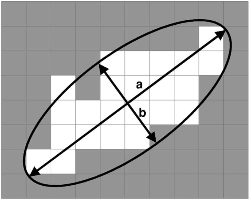
The extraction of the shape features. An ellipse is fitted to the segmented microcalcification using a moment method,¹³ and the lengths of the major axis (a) and the minor axis (b) are determined. The eccentricity feature was defined as $\sqrt{a^2-b^2}/a$, and the axis ratio feature was defined as a/b. The moment ratio feature was defined as the ratio of the smaller second moment of the shape to the larger second moment.

Fig. 7.

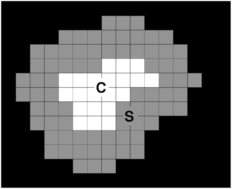
The extraction of the features related to the microcalcification contrast. The white region C at the center represents the segmented microcalcification, and the surrounding gray region S represents the background, obtained by using a dilation operator as described in the text.

After the features were extracted from each microcalcification in a cluster, the mean, standard deviation, maximum, and coefficient of variation of each feature were calculated over each cluster to define cluster features. The number of microcalcifications in a cluster was also defined as a cluster feature. We had 45 morphological features for each cluster.

The texture feature were extracted from regions of interest (ROIs) containing the cluster using the second-order statistics provided by the spatial gray-level dependence (SGLD) matrix.^14,15 The distribution of the SGLD matrix elements reflects the average spatial relationship of pairs of gray-level values with respect to the distance d and direction θ used in SGLD matrix construction. To define the ROI, the bounding box of a detected cluster was enlarged by 5 mm (50 pixels) in each direction so that the background of the surrounding tissue could be included in the analysis. The SGLD matrix was computed in four directions (θ =0°, 45°, 90°, and 135°) and three distances (d=1,2,4) as described in the literature.¹⁵ From each SGLD matrix, 13 texture features related to the distribution of the matrix elements were extracted, namely, energy, correlation, entropy, inertia, inverse difference moment, sum average, sum variance, sum entropy, difference average, difference variance, difference entropy, information measure of correlation 1, and information measure of correlation 2. The formulation of these texture measures has been described in the literature.¹⁶ Two corresponding features in the diagonal direction (θ =45° and 135°) were averaged to yield a single feature. Similarly, two corresponding features in the horizontal and vertical directions (θ =0° and 90°) were also averaged. We thus had a total of 2×3 × 13=78 texture features for each cluster.

The CNN, based on the neocognitron structure of Fukushima,¹⁷ is a backpropagation neural network that operates on images. The input image is filtered by successive nodes in the hidden layers, where each node consists of a group of trainable weights. The output score is a scalar, ideally indicating the likelihood of a true microcalcification in our application. The CNN has been used extensively for the detection of microcalcifications,¹² as well as for detection of lung nodules¹⁸ and mammographic masses.¹⁹ The network architecture and weights were trained previously using a training set that was independent of the data set used in this study.²⁰ In our previous work, the CNN was used for each individual microcalcification before the clustering stage. In this study, we used a low CNN threshold before the clustering stage to exclude only very obvious FPs. After clustering, four CNN score features were extracted for each cluster, namely, the average, standard deviation, maximum, and minimum of the individual microcalcification scores within the cluster. These features were used to define cluster CNN scores to be used for FP reduction.

D. Single-view and similarity classifiers

The above-described features were used in two different classifiers to differentiate true microcalcification clusters from FPs. The first classifier was a single-view classifier that used the features extracted from a cluster on a particular view (CC or MLO). The second classifier was a similarity classifier that jointly used the features of two cluster candidates on two views.

The single-view classifier was trained using stepwise feature selection²¹ and linear discriminant analysis (LDA)²² on the training set. LDA with stepwise feature selection has been previously used in CAD for several applications, including FP reduction for mass detection on mammograms, classification of masses as malignant or benign, classification microcalcification clusters as malignant or benign, and FP reduction for lung nodule detection on CT scans. Stepwise feature selection involves the selection of three parameters, namely, F_in, F_out, and tolerance (tol). A discussion of how these parameters are related to the feature selection process and how they affect the performance can be found in the literature.²¹ In this study, we used a leave-one-case-out method and the area under the receiver operating characteristic curve (A_z) as a figure-of-merit within the training set to determine the best values of these parameters that could provide high classification accuracy with a relatively small number of features. Once they were determined, we used the chosen set of parameters to select a final set of features and LDA coefficients using the entire training set. The feature space available for stepwise selection included 127 features, of which 45 were morphological, 78 were texture, and 4 were CNN score features. Note that only a small subset of the available features will be selected during the classifier design process using the training set.

Our two-view classification algorithm is designed to distinguish between true (TP-TP) pairs and false (FP-TP, TP-FP or FP-FP) pairs by using the similarities between the two objects on different views that constitute the pair. The initial step in this task is to define the object pairs. For a deformable object like the breast under compression, the corresponding locations in the two views cannot be determined exactly based on the two projection mammograms. From the geometry of the mammographic image acquisition, it is known that an object seen on the CC view can appear only in a limited subregion in the MLO view, and vice-versa. Radiologists at our institution routinely use the NOD on the two views to estimate the correspondence between objects seen on different views of the same breast. Based on our previous studies,^3,6 in this work we searched for the member clusters of a pair based on the difference between the NODs on the CC and MLO views. Figure 8 illustrates this geometric pairing procedure. First, the nipple locations N_c and N_m are determined on the CC and MLO views, respectively. Next, the nipple-to-object distance R_c is computed for the cluster candidate C_C1 on the CC view. To find objects on the MLO view to be paired with C_C1, an arc of radius R_c centered at N_m is defined on the MLO view. Next, two concentric arcs, with radii R_c + ΔR and R_c − ΔR are also drawn on the MLO view. Any object that falls within the annular region delineated by these two concentric arcs is paired with the cluster candidate C_C1 on the CC view. In this example, two pairs are defined: C_C1-C_M1 pair and C_C1-C_M2 pair. Although a third cluster candidate C_M3 exists on the MLO view, it is not paired with C_C1 because it falls outside the defined annular region. The half-width of the annular region ΔR is determined using the training data.

Fig. 8.

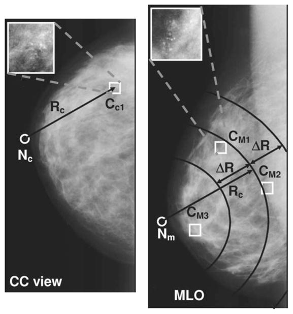
Geometric pairing of the clusters detected on the CC and MLO views. For a cluster C_C1 on the CC view, the nipple-to-object distance R_c is computed. On the MLO view, any object that falls within the annular region delineated by the two concentric arcs R_c + ΔR and R_c − ΔR centered on the nipple location is paired with the cluster candidate C_C1 on the CC view. In this example, two pairs are defined: C_C1-C_M1 pair and C_C1-C_M2 pair. Although a third cluster candidate exists on the MLO view, it is not paired with C_C1 because it falls outside the defined annular region. The half-width ΔR of the annular region is determined using the training data set.

A similarity classifier was designed to score the defined pairs as to their likelihood of being a true pair. For the similarity classifier, two sets of features were generated from the feature set that was used in the single-view classifier. The first set of features consisted of the squared difference of the corresponding features of the two objects in a pair. This set is thus designed to extract the similarity (or dissimilarity) of the features between the detected objects on the two views. For example, one would expect that for a true pair, the average eccentricity of the microcalcifications in the same cluster on the CC and MLO views would be close to each other. For a microcalcification cluster paired with a FP cluster, the difference may be large. The second set of features consisted of the average of the corresponding features. For example, for a true pair, the average CNN score of the individual microcalcifications in the cluster is expected to be large on both views, therefore the corresponding average feature for the pair would also be large. If the microcalcification cluster is paired with a FP cluster, or if two FP clusters are paired, then the CNN score is expected to be small for at least one of the clusters, and therefore the corresponding average feature for the pair would be relatively small. In addition to these two feature sets, we included the NOD difference between the paired clusters as another feature measure. The feature pool for the similarity classifier thus contained a total of 2×127 +1=255 features. The classifier was trained using stepwise feature selection and LDA on the training set, following the same steps described earlier for the single-view classifier.

E. Fusion

The similarity classifier produced a score for each cluster pair. These scores were converted into scores for each individual cluster before being combined with the single-view classifier scores. A cluster on the CC view can be a member of several cluster pairs (paired with more than one cluster on the MLO view), and vice-versa, as illustrated in Fig. 8. The two-view cluster score of a cluster C_i was defined as the maximum of all similarity scores for pairs in which C_i is a member, if that maximum value exceeded a paired-cluster threshold, th_p, determined using the training set. If a cluster C_i was not paired with any cluster on the other view, or if the maximum value was below th_p, then it was assigned a large negative two-view cluster score, chosen arbitrarily as −100 in this study. The idea behind using the paired-cluster threshold th_p is that if a cluster is geometrically paired with a cluster on the other view, but the evidence for the similarity of the two clusters is weak, then it is likely a false pair and may be eliminated.

By using a constant paired-cluster threshold, and varying the decision threshold on the similarity scores, one can obtain a FROC curve for the detection of microcalcification clusters. Since this detection method uses only the paired information from the two mammographic views, it is termed the exclusive two-view detection method in the following discussion. To utilize both the one-view and two-view information, an effective fusion method has to be designed. In this study, we found that good fusion performance could be achieved for a cluster by averaging its single-view score and exclusive two-view detection score.

F. Evaluation

The accuracy of the single-view and similarity classifiers was evaluated using ROC analysis.²³ A cluster was considered to be a TP if its bounding-box overlapped the radiologist-defined microcalcification location by more than 40%. Other detected clusters were considered as FPs. The overall detection accuracy of the two systems was compared using free response ROC (FROC) analysis. The sensitivity axis in FROC analysis was based on the positive data set. The number of FPs per mammogram was estimated using the normal data set. For the test set, we plotted two types of FROC curves, using mammogram-based and cased-based analyses. In the mammogram-based analysis, the same cluster seen on two views are counted independently. A TP was defined as a true microcalcification cluster detected by the computer. Since there were 218 microcalcification cluster locations marked by the radiologist on the test set, the denominator for sensitivity in mammogram-based analysis was 218. If a radiologist-marked cluster was detected as more than one cluster by the computer, they would be counted only as one TP. In the case-based analysis, a TP was defined as a positive case for which a cluster was correctly detected on one or both views. Since we had 96 mammogram pairs in our positive test set, the denominator for sensitivity in case-based analysis was 96. If more than one TP cluster was detected for a case, this was counted as only one TP.

III. RESULTS

The prescreening algorithm detected an average of 3.06 clusters per mammogram in the normal training (USF) group, and 4.11 clusters in the normal test (UM) group. On the positive training (USF) group, 89% (226/254) of the true cluster locations were detected by prescreening, while the corresponding sensitivity for the positive test (UM) group was 93% (202/218).

To determine the parameters to be used in feature selection for the single-view classifier, we used a leave-one-case-out method within the training set. Mammograms corresponding to each case were left out once as a validation sample, feature selection and LDA design were performed on the rest of the training set, and the LDA scores were obtained for the clusters in the validation samples. After the validation scores were obtained for each case, these scores were pooled and an A_z value was derived from ROC analysis. Table II shows the average number of selected features and the validation A_z values obtained using the leave-one-case-out method on the training set for different values of the parameters used in feature selection. It can be seen that the A_z value was not very sensitive to these parameters in the range that we studied. The parameters for feature selection were therefore selected as F_in=9.4, F_out=9.2, and tol=0.01, which provided the highest A_z with the smallest number of features. When these parameters were applied to the entire training set, a total of 8 features were selected. Four of these were CNN features, two were texture features, two were contrast features, and one was the number of microcalcifications.

Table II.

The area A_z under the ROC curve and the number of selected features for different values of stepwise feature selection parameters used in the design of the one-view classifier. The area A_z was obtained from the left-out validation samples in a leave-one-case-out resampling within the training data set. The number of selected features represents the average number of selected features in each cycle of the leave-one-out process.

Fin	Fout	Tol	Az	Number of selected features
9.4	9.2	0.0001	0.89±0.01	8
9.4	9.2	0.01	0.89±0.01	8
11.4	11.2	0.0001	0.88±0.01	7
11.4	11.2	0.01	0.88±0.01	7
7.4	7.2	0.0001	0.89±0.01	9
7.4	7.2	0.01	0.89±0.01	9
5.4	5.2	0.0001	0.87±0.01	12
5.4	5.2	0.01	0.87±0.01	11

Figure 9 shows the NOD differences for the CC and MLO view mammograms for the positive training and test data sets. Based on the histogram of the training data set, we selected ΔR=26 mm for the geometric pairing of the data. As can be observed from Fig. 9, this choice for ΔR resulted in 4 true missed pairs on the training set, and 5 true missed pairs on the test set. On the other hand, a large fraction of false pairs were eliminated. For the training set, there were a total of 2843 pairs that could be defined on the normal mammograms without the geometric constraint. The geometric pairing using ΔR=26 mm eliminated 62% (1750/2843) of these pairs, resulting in 1093 false pairs. Similarly, for the normal test set, the geometric pairing eliminated 61% (1183/1943) of the possible false pairs, resulting in 760 pairs.

Fig. 9.

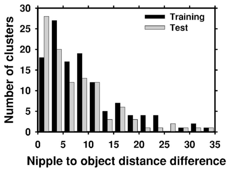
The distribution of the NOD differences for the true cluster centroids on the CC and MLO views. Based on the distribution of the NOD differences for the training data set, the half-width ΔR of the annular region was selected as ΔR=26 mm.

The feature selection parameters for the similarity classifier were also determined using a leave-one-case-out method within the training set. Table III shows the average number of selected features and the validation A_z values obtained using the leave-one-case-out method on the training set for different values of the parameters used in feature selection. Similar to the results for the single-view classifier, the A_z value was not very sensitive to the feature selection parameters in the range that we studied. Based on these results, the parameters for feature selection were chosen as F_in=35.4, F_out=35.2, and tol=0.01. When these parameters were applied to the entire training set, a total of 13 features were selected, of which 8 were squared difference features and 5 were average features. Of the squared difference features, three were from contrast features, two from CNN features, one from a texture feature, one from a shape feature, and one from the number of microcalcifications. Of the average features, two were contrast features, one was a CNN feature, one was a texture feature, and one was the number of microcalcifications.

Table III.

The area A_z under the ROC curve and the number of selected features for different values of stepwise feature selection parameters used in the design of the two-view classifier. The area A_z was obtained from the left-out validation samples in a leave-one-case-out resampling within the training data set. The number of selected features represents the average number of selected features in each cycle of the leave-one-out process.

Fin	Fout	tol	Az	Number of selected features
35.4	35.2	0.0001	0.96±0.003	13
35.4	35.2	0.01	0.96±0.003	13
45.4	45.2	0.0001	0.95±0.003	10
45.4	45.2	0.01	0.95±0.003	9
25.4	25.2	0.0001	0.96±0.003	16
25.4	25.2	0.01	0.96±0.003	16
15.4	15.2	0.0001	0.96±0.003	18
15.4	15.2	0.01	0.96±0.003	18
5.4	5.2	0.0001	0.95±0.003	47
5.4	5.2	0.01	0.95±0.004	37

To select the paired-cluster threshold, the resubstitution FROC curves for the training set were plotted for different selected values of the threshold. Figure 10 shows these FROC curves for five of the selected thresholds. Based on these plots, the paired-cluster threshold was selected as th_p =0.0.

Fig. 10.

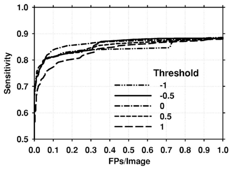
Mammogram-based resubstitution FROC curves for different values of the paired-object threshold th_p. Based on these FROC curves, the paired-cluster threshold was selected as th_p =0.

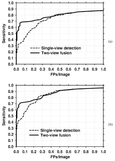
The designed classifiers were applied to the test set. Figure 11 presents the mammogram-based test FROC curves for the single-view and exclusive two-view detection methods. The comparison shows that the exclusive two-view detection method had a very low FP rate for the test set at low sensitivity. However, the highest per-film sensitivity that could be reached by exclusive two-view detection was 69%. In contrast, single-view detection could reach a sensitivity of 93% (not shown in the figure), but at a high FP rate. Figure 12(a) shows the FROC curve when the scores of these two classifiers were fused. The result indicates that at relatively high FP rates, the two-view fusion classifier behaved essentially as the single-view classifier. However, at lower FP rates, the sensitivity of the two-view fusion classifier was much higher. To study whether the improvement was significant, we applied JAFROC analysis.²⁴ The figure-of-merit (FOM) from the output of the JAFROC software was 0.85 and 0.81, respectively, for two-view fusion and single-view detection. The difference between the FOM was statistically significant (p=0.0002). Figure 12(b) compares the case-based FROC curves for the single-view detection and two-view fusion approach. It can be seen again that two-view fusion resulted in a higher FROC curve.

Fig. 11.

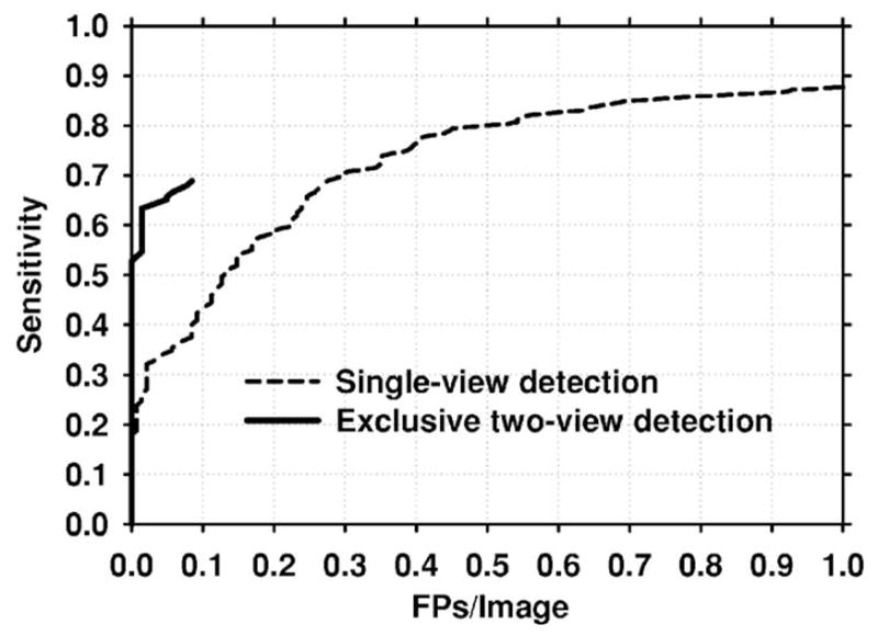
Mammogram-based test FROC curves for the single-view and exclusive two-view detection methods. The exclusive two-view detection method had a very low FP rate, but could only reach a maximum sensitivity of 69%. The single-view detection method had a higher maximum sensitivity, but had a higher FP rate than the exclusive two-view detection method at low sensitivity.

Fig. 12.

FROC curves for the single-view and two-view fusion methods for the entire test data set. (a) Mammogram-based, (b) Case-based.

The improvement with two-view fusion was also analyzed for the subsets of malignant and benign test cases. Figures 13(a) and 13(b) compare the single-view and two-view fusion methods for the malignant cases using mammogram-based and case-based analysis, respectively. Figures 14(a) and 14(b) present the corresponding curves for the benign cases. The detection performance with both single-view detection and two-view fusion is higher for malignant clusters than for benign clusters. Two-view fusion results in a greater improvement in performance for malignant clusters than for benign clusters. The improvement with two-view fusion was found to be significant for both malignant (p=0.0007) and benign (p=0.0013) clusters using JA-FROC analysis. Table IV compares the FP rates for single-view detection and two-view fusion at selected sensitivities for the entire data set, the subset of malignant clusters, and the subset of benign clusters.

Fig. 13.

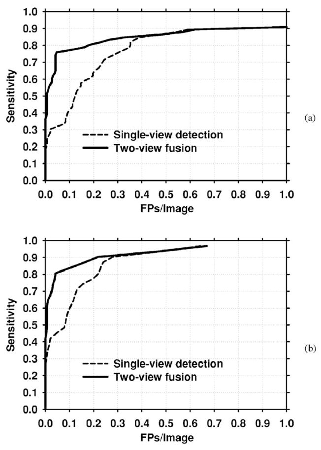
FROC curves for the malignant test set. (a) Mammogram-based, (b) Case-based.

Fig. 14.

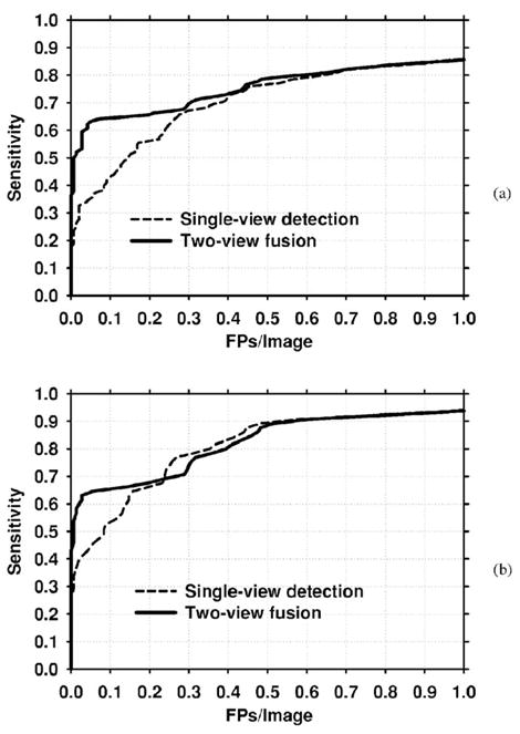
FROC curves for the benign test set. (a) Mammogram-based, (b) Case-based.

Table IV.

The average number of FPs at selected sensitivities for the single-view and two-view fusion detection methods. The average number of FPs is compared for the entire test data set, as well as the malignant and benign subsets. For computing the sensitivity in mammogram-based scoring, the same cluster seen on two views was counted independently. Since there were 218 microcalcification cluster locations marked by the radiologist on the test set, the denominator for sensitivity in mammogram-based analysis was 218. In case-based analysis, a TP was defined as a positive case for which a cluster was correctly detected on one or both views. Since we had 96 mammogram pairs in our data positive test set, denominator for sensitivity in case-based analysis was 96.

Scoring method	Data subset	Average number of FPs per image
		80% sensitivity		70% sensitivity
		Single-view	Fusion	Single-view	Fusion
Mammogram-based	Entire test set	0.53	0.46	0.30	0.18
	Malignant	0.35	0.16	0.24	0.04
	Benign	0.63	0.56	0.37	0.30
Case-based	Entire test set	0.26	0.30	0.17	0.04
	Malignant	0.22	0.04	0.13	0.03
	Benign	0.35	0.39	0.24	0.25

We also studied whether two-view fusion would be effective when the training and test sets were switched. For this purpose, we designed the single-view and similarity classifiers and the paired-cluster threshold using the UM data set, and applied the designed classifiers to the USF data set. The resulting mammogram-based FROC curves are shown in Fig. 15. The FROC curve for the two-view fusion classifier is again higher than that of the single-view classifier. At 80% sensitivity, the single-view and the two-view fusion classifiers had an average FP rate of 0.18 and 0.06 FPs/mammogram, respectively. It is also observed that these FP rates are lower than the corresponding mammogram-based rates obtained using the UM data set as the test set (Table IV).

Fig. 15.

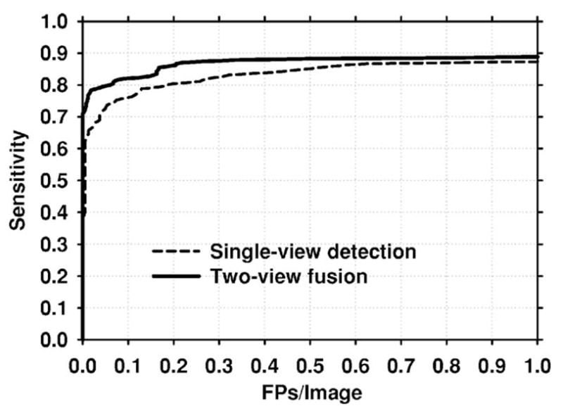
Single-view and two-view fusion mammogram-based test FROC curves when the training and test sets are switched. To obtain these curves, classifiers were trained on the UM data set. The trained classifiers were then applied to the USF data set.

IV. DISCUSSION

Our results indicate that the two-view classifier and the fusion of the two-view scores with single-view scores improved the microcalcification detection accuracy of our CAD system. A significant improvement in the mammogram-based test FROC curves was achieved using two-view fusion compared to single-view detection. Much of this improvement resulted from the lower FP rates of our similarity classifier at lower sensitivities. At high sensitivity (above 80%), the mammogram-based FROC curves of the two-view fusion and single-view detection methods were almost identical. The improvement was also significant for the subsets of malignant and benign clusters of our test data set.

There were 104 microcalcification clusters seen on both views in the abnormal test group. Of these, 90 (87%) were matched with the corresponding cluster after geometric pairing. Of the 14 missed matches, five were caused by the absolute value of the NOD being larger than ΔR=26 mm, and the remaining nine were caused by either one or both of the clusters being missed by the prescreening algorithm. The paired-cluster threshold, th_p, eliminated an additional 16 matches, resulting in a total of 74 correctly matched microcalcification clusters for the exclusive two-view detection. The highest sensitivity of exclusive two-view detection was 69% (150/218), because the scores of two of the true clusters that were matched with false clusters in the corresponding view were above th_p. In return for missing 16 out of a total of 104 true cluster pairs (15% miss), a substantial number of FP pairs were eliminated with the use of the paired-cluster threshold. After geometric pairing, we had a total of 760 false pairs in the normal test group. The use of the paired-cluster threshold eliminated 754 of these, resulting in a total of only 6 false pairs, or an average of 0.08 (12/142) FP clusters/normal image.

The paired-cluster threshold in this study was determined using the training set as th_p =0. To evaluate the effect of this threshold on the test results, we also obtained test FROC curves for different values of th_p. The curves for th_p =0.5, 0, −0.5, −1, and −2 are shown in Fig. 16. It is observed that the FROC curve may be higher if thresholds lower than that obtained by training were used. However, as seen in Fig. 10, a lower threshold than th_p =0 resulted in worse performance for the training set. Since the parameters of a CAD system ought to be selected using the training set, and not by comparing the test performance for different parameters, we maintain that unbiased test results are those found by using th_p =0 (Fig. 12).

Fig. 16.

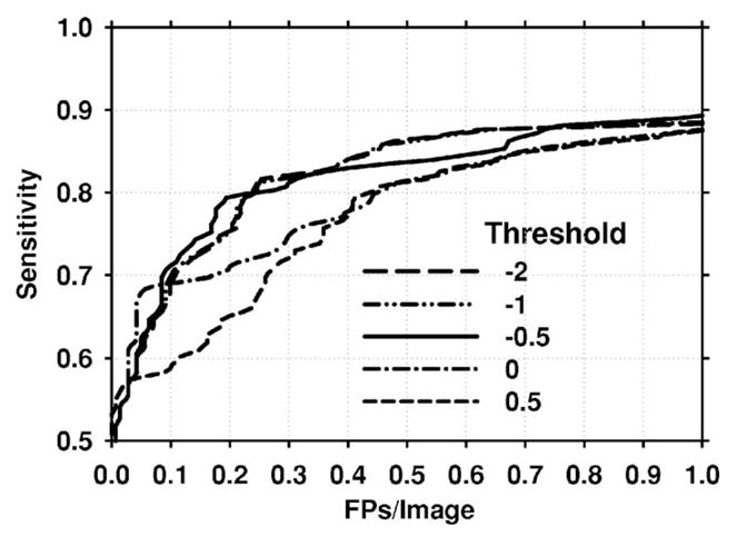
Mammogram-based FROC curves for different values of the paired-clusters threshold th_p. When the value of th_p was set to less than that obtained by training (th_p <0) the FROC curves for the test set were higher than the test FROC curve obtained with th_p =0, which was determined by training.

Comparing mammogram-based test FROC curves with case-based curves, we find that the improvement with two-view fusion is more limited for case-based detection. Figures 12(a) and 14(a) demonstrate that single-view detection may provide slightly lower FP rate for some sensitivity values when case-based scoring is employed. However, at low sensitivity, case-based two-view fusion FROC curves are substantially higher. Since there is currently no accepted method to compare case-based FROC curves, we did not evaluate the statistical significance in the difference between these curves.

Comparing the test FROC curves in Figs. 12(a) and 15, we found that the detection performance for the USF and UM sets are different. For example, at a sensitivity of 85%, the average number of FPs for the USF and UM data sets are 0.17 and 0.71, respectively. Part of this difference may be attributed to the fact that the USF data set contained biopsy-proven malignant cases, whereas the UM data set contained a mixture of malignant and benign clusters. A comparison of the FROC curves for malignant and benign subsets of the UM data set (Figs. 13 and 14) indicates that the CAD system has a higher detection accuracy for malignant microcalcification clusters. However, this does not completely explain the difference between Figs. 12(a) and 15. Figures 13(a) and 15 show that the detection accuracy for the USF data set is higher than that of the malignant UM subset. For example, at a sensitivity of 85%, the average number of FPs for the USF and malignant UM data sets are 0.17 and 0.33, respectively. This indicates that the UM data set may contain more difficult cases than the USF data set. The subtlety ratings of the USF (Fig. 2) and UM (Fig. 4) cases also indicate that the UM cases may be more subtle, although the subtlety rating scales are subjective and may not be easily compared among radiologists. These differences also underscore the difficulty of comparing the performances for algorithms evaluated with data sets collected at different institutions.

Our study had a number of limitations. The nipple locations in our study were hand-extracted. Therefore, the two-view detection process was not entirely automated. We have been developing automated nipple detection methods on mammograms.²⁵ Joint two-view detection with automatically identified nipple locations will be studied in the future. Cases containing diffuse microcalcifications and calcified vessels were excluded from both the training and test data sets because of the difficulty of establishing the correspondence of the clusters on the two views. If the two-view detection method were applied to cases containing diffuse microcalcifications, a large number of TP pairs would be identified. Although it may be impossible to judge which pairs truly correspond to each other, it is quite likely that some of the pairs will attain a high two-view score, and thus result in a correct detection. If the two-view detection method were applied to normal cases containing calcified vessels, again a large number of FP pairs would be detected. A reasonable method to handle cases containing calcified vessels may be to automatically identify such vessels after preprocessing, apply only single-view detection, and mark the detected calcified vessels in a special way (e.g., different color than other detections). In this study, we did not attempt any type of automated detection for calcified vessels.

A number of parameters in this study were optimized based on the training set, such as the feature selection thresholds in the LDA design and the paired-cluster threshold. However, we did not perform a joint optimization of many other parameters, such as the width of the annular region used in geometric pairing, the thresholds used in prescreening, or the weights for fusion of the two classifiers. A methodical optimization of the large number of parameters in the single-view and two-view detection algorithms may improve the final classification accuracy. Any improvement in the geometric pair definition will also improve the joint two-view detection.

V. CONCLUSION

We have developed a joint two-view detection method to improve the computerized detection of microcalcification clusters on two-view mammograms. A geometric method was used to pair the clusters from the two views. A two-view classifier was designed to distinguish between true and false pairs by using the similarities between the two clusters on different views that constitute the pair. The scores of the two-view similarity classifier were fused with the single-view cluster scores obtained from a conventional classifier designed for differentiating true and false clusters on one view. Our results indicate that two-view fusion may significantly reduce FP clusters and improve the FROC curve of microcalcification detection for both malignant and benign clusters. The improvement for malignant clusters was more substantial than that for benign clusters. Directions for future work include automated identification of nipple locations, and optimization of parameters used in single-view and two-view detection.

References

- 1.Thurfjell E, Taube A, Tabar L. One-view versus 2-view mammography screening—A prospective population-based study. Acta Radiol. 1994;35:340–344. [PubMed] [Google Scholar]
- 2.Warren R, Duffy S, Bashir S. The value of the second view in screening mammography. Br J Radiol. 1996;69:105–108. doi: 10.1259/0007-1285-69-818-105. [DOI] [PubMed] [Google Scholar]
- 3.Paquerault S, Petrick N, Chan HP, Sahiner B, Helvie MA. Improvement of computerized mass detection on mammograms: Fusion of two-view information. Med Phys. 2002;29:238–247. doi: 10.1118/1.1446098. [DOI] [PubMed] [Google Scholar]
- 4.Sahiner B, Gurcan MN, Chan HP, Hadjiiski LM, Petrick N, Helvie MA. The use of joint two-view information for computerized lesion detection on mammograms: Improvement of microcalcification detection accuracy. Med Phys. 2002;4684:754–761. [Google Scholar]
- 5.Paquerault S, Petrick N, Chan HP, Sahiner B, Dolney AY. Improvement of mammographic lesion detection by fusion of information from different views. Proc SPIE. 2001;4322:1883–1889. [Google Scholar]
- 6.Paquerault S, Sahiner B, Petrick N, Hadjiiski LM, Gurcan MN, Zhou C, Helvie MA. Prediction of Object Location in Different Views Using Geometrical Models. Vol. 2001. Toronto, Canada: Medical Physics; Madison, WI: 2001. pp. 748–755. [Google Scholar]
- 7.Yam M, Brady M, Highnam R, Behrenbruch C, English R, Kita Y. Three-dimensional reconstruction of microcalcification clusters from two mammographic views. IEEE Trans Med Imaging. 2001;20:479–489. [PubMed] [Google Scholar]
- 8.Kita Y, Highnam RP, Brady JM. Correspondence between different view breast X rays using curved epipolar lines. Comput Vis Image Underst. 2001;83:38–56. [Google Scholar]
- 9.Chang YH, Good WF, Sumkin JH, Zheng B, Gur D. Computerized localization of breast lesions from two views—An experimental comparison of two methods. Invest Radiol. 1999;34:585–588. doi: 10.1097/00004424-199909000-00006. [DOI] [PubMed] [Google Scholar]
- 10.Heath M, Bowyer K, Kopans D, Kegelmeyer P, Moore R, Chang K, Munishkumaran S. In: Digital Mammography. Karssemeijer N, Thijssen M, Hendriks J, van Erning L, editors. Kluwer Academic; Dordrecht: 1998. pp. 457–460. [Google Scholar]
- 11.Chan HP, Doi K, Vyborny CJ, Schmidt RA, Metz CE, Lam KL, Ogura T, Wu Y, MacMahon H. Improvement in radiologists, detection of clustered microcalcifications on mammograms. The potential of computer-aided diagnosis. Invest Radiol. 1990;25:1102–1110. doi: 10.1097/00004424-199010000-00006. [DOI] [PubMed] [Google Scholar]
- 12.Chan HP, Lo SCB, Sahiner B, Lam KL, Helvie MA. Computer-aided detection of mammographic microcalcifications: Pattern recognition with an artificial neural network. Med Phys. 1995;22:1555–1567. doi: 10.1118/1.597428. [DOI] [PubMed] [Google Scholar]
- 13.Chan HP, Sahiner B, Lam KL, Petrick N, Helvie MA, Goodsitt MM, Adler DD. Computerized analysis of mammographic microcalcifications in morphological and texture feature space. Med Phys. 1998;25:2007–2019. doi: 10.1118/1.598389. [DOI] [PubMed] [Google Scholar]
- 14.Haralick RM, Shanmugam K, Dinstein I. Texture features for image classification. IEEE Trans Syst Man Cybern. 1973;SMC-3:610–621. [Google Scholar]
- 15.Chan HP, Sahiner B, Petrick N, Helvie MA, Leung KL, Adler DD, Goodsitt MM. Computerized classification of malignant and benign microcalcifications on mammograms: Texture analysis using an artificial neural network. Phys Med Biol. 1997;42:549–567. doi: 10.1088/0031-9155/42/3/008. [DOI] [PubMed] [Google Scholar]
- 16.Wei D, Chan HP, Petrick N, Sahiner B, Helvie MA, Adler DD, Goodsitt MM. False-positive reduction technique for detection of masses on digital mammograms: Global and local multiresolution texture analysis. Med Phys. 1997;24:903–914. doi: 10.1118/1.598011. [DOI] [PubMed] [Google Scholar]
- 17.Fukushima K, Miyake S, Ito T. Neocognitron: A neural network model for a mechanism of visual pattern recognition. IEEE Trans Syst Man Cybern. 1983;SMC-13:826–834. [Google Scholar]
- 18.Lo SC, Lou SL, Lin JS, Freedman MT, Mun SK. Artificial convolution neural network techniques and applications to lung nodule detection. IEEE Trans Med Imaging. 1995;14:711–718. doi: 10.1109/42.476112. [DOI] [PubMed] [Google Scholar]
- 19.Sahiner B, Chan HP, Petrick N, Wei D, Helvie MA, Adler DD, Goodsitt MM. Classification of mass and normal breast tissue: A convolution neural network classifier with spatial domain and texture images. IEEE Trans Med Imaging. 1996;15:598–610. doi: 10.1109/42.538937. [DOI] [PubMed] [Google Scholar]
- 20.Gurcan MN, Sahiner B, Chan HP, Hadjiiski LM, Petrick N. Selection of an optimal neural network architecture for computer-aided detection of microcalcifications—Comparison of automated optimization techniques. Med Phys. 2001;28:1937–1948. doi: 10.1118/1.1395036. [DOI] [PubMed] [Google Scholar]
- 21.Draper NR. Applied Regression Analysis. Wiley; New York: 1998. [Google Scholar]
- 22.Lachenbruch PA. Discriminant Analysis. Hafner; New York: 1975. [Google Scholar]
- 23.Swets JA. ROC analysis applied to the evaluation of medical imaging techniques. Invest Radiol. 1979;14:109–121. doi: 10.1097/00004424-197903000-00002. [DOI] [PubMed] [Google Scholar]
- 24.Chakraborty DP, Berbaum KS. Observer studies involving detection and localization: Modeling, analysis, and validation. Med Phys. 2004;31:2313–2330. doi: 10.1118/1.1769352. [DOI] [PubMed] [Google Scholar]
- 25.Zhou C, Chan HP, Paramagul C, Roubidoux MA, Sahiner B, Hadjiiski LM, Petrick N. Computerized nipple identification for multiple image analysis in computer-aided diagnosis. Med Phys. 2004;31:2871–2882. doi: 10.1118/1.1800713. [DOI] [PMC free article] [PubMed] [Google Scholar]