Initial Evaluation of Direct 4D Parametric Reconstruction with Human PET Data

Abstract

Previously, we presented a direct EM method for producing kinetic parameter images from list mode PET data, where the time-activity curve for each voxel is described by a one-tissue compartment model (1T). The initial evaluations were performed with simulations, without motion, randoms, or scatter effects included. By extension of our previous frame-based physics correction methods, a practical direct 4D parametric reconstruction algorithm is now proposed and implemented for human data. Initial evaluations were performed using 3 human subjects with the serotonin transporter tracer [¹¹C]AFM. Comparisons with the 2-step approach (frame-based reconstruction followed by voxel-by-voxel parameter estimation) provided encouraging initial results. Regional analysis showed that the 2-step and 4D methods have similar K₁ and V_T values, but with a consistent difference. Visual analysis showed some noise reduction in 4D. These initial results suggest that direct 4D parametric reconstruction can be performed with real data, and offers the potential for improved accuracy and precision over the 2-step frame method.

I. Introduction

Dynamic positron emission tomography (PET) permits quantification of tracer dynamics. The current two-step frame-based approach is to 1) reconstruct a time series of images from measured projection data independently, and 2) fit the voxel time-activity curves to a kinetic model. This process requires selection of the duration of each frame, involving a choice between collecting longer frames with better counting statistics but poor temporal resolution, or shorter frames that are noisier, but preserve the temporal resolution. Optimal use of these dynamic data requires accurate noise estimates for data weighting; this estimation is challenging for nonlinear iterative reconstruction methods because voxel and ROI noise is spatially variant and object dependent.

Many promising direct approaches [1–8] for parametric image creation have been proposed, which directly use full dynamic data in a unified estimation and have the potential to improve statistical quality, resolution uniformity, and reduce bias and variability. Carson and Lange [1] proposed a general EM framework for direct parametric image reconstruction algorithm with nonlinear kinetic model. The method of Reader et al [2] was developed from linear basis functions, whose the temporal model is linear with respect to the parameters. Although such basis functions can represent the TAC, they have no direct physiological meaning and kinetic parameters must still be calculated from the dynamic images, leading again to a two-step process. The application of kinetic compartment models is more biologically based, and is the primary goal of dynamic PET. Wang et al [4] and Tsoumpas et al [6] proposed direct parametric image reconstruction methods, for a compartment model which is linear (Patlak plot), and is thus limited to irreversible tracers such as FDG. Furthermore, Rahmim et al [7] proposed a closed-form direct 4D parametric image estimation method for the reversible tracer with the help of recently published linear graphical analysis model. Kamasak et al [3] developed a direct parametric iterative coordinate descent algorithm for two-tissue compartmental model from sinogram data. Recently, Wang and Qi [5] proposed a generalized direct parametric image reconstruction approach applicable to any kinetic model, which was comprised of two steps for each parameter update (reconstruction of intermediate images and kinetic parameter estimation with accurate weights determined from the derived algorithm). Independently, we presented a new EM-based direct parametric image reconstruction algorithm [8] for list mode data by combining the nonlinear one tissue (1T) compartment model into the physical model and built this algorithm into our MOLAR software [9]. In simulations, we showed accurate estimation with less variance compared to the frame-based method. In this comparison, we carefully selected the weighting of the frames in order to optimize its performance

In quantitative PET, corrections for randoms and scatter are required to produce accurate results. In conventional frame-based reconstruction, these corrections are typically performed on a frame-by-frame basis. However, for 4D reconstruction, a continuous estimate of the randoms and scatter rates is required. In MOLAR, continuous estimates of these values are produced as follows:

Random Correction

Randoms R_i are estimated from the known timing window (τ) and the single rates of the 2 crystals (S₁, S₂) that produce LOR k with the formula R_i=2τS₁S₂. Crystal singles rates are obtained by multiplying block singles rates stored in the list mode file by the ratio of the individual crystal efficiency to the total efficiency of the block; these efficiencies are derived from the component-based normalization. Delayed coincidences in the list mode stream are not used in the reconstruction, except to validate the random estimates. Thus, this approach permits continuous estimates of randoms.

Scatter correction

Scatter estimation was performed using the single-scatter simulation (SSS) method of Watson [10]. This method was implemented iteratively within the reconstruction algorithm, i.e., the scatter estimate was determined three times, each with an updated emission image. For the cluster-based reconstruction, calculations for each scatter point are distributed across different processors.

For scatter estimation, the scatter rate is proportional to the sum of the contributions from scatter points randomly positioned in the attenuation volume, and thus depends on the emission image. In the frame method, each frame’s emission image is static and the LOR scatter rate is time independent. Further, the absolute scatter rate for each LOR is determined by scaling the simulated scatter profiles based on the LOR values immediately outside the object (after randoms correction), so initially the scatter estimation was a frame-based operation. However, in the direct 4D mode, the emission image (and potentially the scatter scale factor) is time-varying, so the frame-based SSS method cannot be employed to produce a continuous scatter estimate. Here, we present a practical SSS method for the 4D method to provide a scatter estimate that is continuous in time. Using this method, we show initial evaluation of the 4D EM method for human data.

II. Theory

A. Direct 4D Parametric Imaging Algorithm

We extend the previous K₁ and k₂ update equations [8] by including attenuation, live time, decay, normalization, motion effects, random and scattered coincidences:

$$H\left(k_{2j}\right)=\frac{{\displaystyle \sum _{i=1}^I}{\displaystyle \sum _{t=0}^T}{\displaystyle \sum _{\tau =0}^t}\mathrm{\Delta }t{c}_{\mathit{ijt}}{L}_{it}{A}_{it}{N}_i{P}_{\tau }{e}^{-k_{2j}(t-\tau )}(t-\tau )}{{\displaystyle \sum _{i=1}^I}{\displaystyle \sum _{t=0}^T}{\displaystyle \sum _{\tau =0}^t}\mathrm{\Delta }t{c}_{\mathit{ijt}}{L}_{it}{A}_{it}{N}_i{P}_{\tau }{e}^{-k_{2j}(t-\tau )}}$$ (1)

$$M_{\mathit{ijt}\tau }^{(n)}=Y_{it}\frac{\mathrm{\Delta }t{c}_{\mathit{ijt}}{L}_{it}{A}_{it}{N}_i{K}_{1j}^{(n)}{P}_{\tau }{e}^{-k_{2j}^{(n)}(t-\tau )}}{\mathrm{\Delta }t\left(\left({\displaystyle \sum _{j^{\prime }=1}^J}{\displaystyle \sum _{{\tau }^{\prime }=0}^t}{c}_{i{j}^{\prime }t}{L}_{it}{A}_{it}{N}_i{K}_{1j^{\prime }}^{(n)}{P}_{{\tau }^{\prime }}{e}^{-k_{2j^{\prime }}^{(n)}(t-{\tau }^{\prime })}\right)+R_{it}+S_{it}\right)}$$ (2)

$$k_{2j}^{(n+1)}=H^{-1}\left(\frac{{\displaystyle \sum _{i=1}^I}{\displaystyle \sum _{t=0}^T}{\displaystyle \sum _{\tau =0}^t}(t-\tau )M_{\mathit{ijt}\tau }^{(n)}}{{\displaystyle \sum _{i=1}^I}{\displaystyle \sum _{t=0}^T}{\displaystyle \sum _{\tau =0}^t}{M}_{\mathit{ijt}\tau }^{(n)}}\right)$$ (3)

$$K_{1j}^{(n+1)}=\frac{{\displaystyle \sum _{i=1}^I}{\displaystyle \sum _{t=0}^T}{\displaystyle \sum _{\tau =0}^t}{M}_{\mathit{ijt}\tau }^{(n)}}{\mathrm{\Delta }t\left({\displaystyle \sum _{i=1}^I}{\displaystyle \sum _{t=0}^T}{\displaystyle \sum _{\tau =0}^t}{c}_{\mathit{ijt}}{L}_{it}{A}_t{N}_i{P}_{\tau }{e}^{-k_{2j}^{(n+1)}(t-\tau )}+R_{it}+S_{it}\right)}$$ (4)

where Eq. 1 defined H(k₂), the nonlinear function relating k₂ and the input function to the measured data. Eq. 2 is the conditional expectation of the spatial-temporal complete data given the current kinetic parameter estimate (K₁⁽ⁿ⁾ and k₂⁽ⁿ⁾) and measured data (Y), Eq. 3 is update equation for k₂, and Eq. 4 is the update equation for K₁. In these equations, i is the LOR index, j is the voxel index, and t is the continuous time index. c_ijt is the probability of an emission from voxel j detected on line of response (LOR) i in time bin t. L_it is product of live time and decay factor. A_it is attenuation factor on LOR i in time bin t. N_i is normalization factor on LOR i. Y_it, R_it and S_it are the counts detected, random and scatter estimates on LOR i in time bin t. P_t is the plasma input function. For list mode, time bins have 1-msec duration, i.e., the time resolution of the list mode data.

In the presence of continuous motion, the direct computation of H(k_2j) is extremely computationally intensive. If motion effects in H(k_2j) are ignored, Eq. 2 can be simplified to:

$$H\left(k_{2j}\right)=\frac{{\displaystyle \sum _{t=0}^T}{\displaystyle \sum _{\tau =0}^t}{D}_t{P}_{\tau }{e}^{-k_{2j}(t-\tau )}(t-\tau )}{{\displaystyle \sum _{t=0}^T}{\displaystyle \sum _{\tau =0}^t}{D}_t{P}_{\tau }{e}^{-k_{2j}(t-\tau )}}$$ (5)

which can be pre-calculated given the blood input function and the decay model (D_t=exp(−ln2*t/t_1/2)), where t_1/2 is half life of tracer.

B. SSS for Direct 4D

For SSS, the expected scatter rate between detectors A and B is estimated as:

$$S^{AB}=\underset{V_s}{\int }d{V}_s\left(\frac{{\sigma }_{AS}{\sigma }_{BS}}{4\pi R_{AS}^2{R}_{BS}^2}\right)\frac{\mu }{{\sigma }_c}\frac{d{\sigma }_c}{d\mathrm{\Omega }}\left[I^A+I^B\right]$$ (6)

where:

$$I^A={\epsilon }_{AS}{\epsilon }_{BS}^{\prime }{e}^{-\left(\underset{S}{\overset{A}{\int }}\mu d_s+\underset{S}{\overset{B}{\int }}{\mu }^{\prime }{d}_s\right)}\underset{S}{\overset{A}{\int }}\lambda (s)ds$$ (7)

$$I^B={\epsilon }_{BS}{\epsilon }_{AS}^{\prime }{e}^{-\left(\underset{S}{\overset{B}{\int }}\mu d_s+\underset{S}{\overset{A}{\int }}{\mu }^{\prime }{d}_s\right)}\underset{S}{\overset{A}{\int }}\lambda (s)ds$$ (8)

In MOLAR’s implementation of SSS, a coarsely-sampled spatial grid of scatter points is used. Likewise, the scatter projection space is also coarsely sampled (after uniform sampling, the number of transaxial crystals is 100 and the number of axial crystals is 17) and the scatter estimate for any LOR is interpolated from this sampled space. In addition, the scatter estimate is scaled with a global factor obtained by matching the calculated scatter estimate to the scatter measured (prompts-delays) outside the attenuation volume. The scatter estimate is not pre-computed but calculated iteratively from the estimate of emission image at several subsets (0, 4 and 10) during the first iteration.

In the direct 4D method, the scatter rate is time dependent, I^A and I^B are replaced by I^A(t) and I^B(t) respectively:

$$\begin{array}{l}{I}^A\left(t\right)={\epsilon }_{AS}{\epsilon }_{BS}^{\prime }{e}^{-\left(\underset{S}{\overset{A}{\int }}\mu d_s+\underset{S}{\overset{B}{\int }}{\mu }^{\prime }{d}_s\right)}\underset{S}{\overset{A}{\int }}\lambda \left(s,t\right)ds\\ ={\epsilon }_{AS}{\epsilon }_{BS}^{\prime }{e}^{-\left(\underset{S}{\overset{A}{\int }}\mu d_s+\underset{S}{\overset{B}{\int }}{\mu }^{\prime }{d}_s\right)}\underset{S}{\overset{A}{\int }}{K}_1\left(s\right)\sum _{\tau }{P}_{\tau }{e}^{-k_2(s)(t-\tau )}ds\end{array}$$ (9)

$$\begin{array}{l}{I}^B(t)={\epsilon }_{BS}{\epsilon }_{AS}^{\prime }{e}^{-\left(\underset{S}{\overset{B}{\int }}\mu d_s+\underset{S}{\overset{A}{\int }}{\mu }^{\prime }{d}_s\right)}\underset{S}{\overset{B}{\int }}\lambda \left(s,t\right)ds\\ ={\epsilon }_{BS}{\epsilon }_{AS}^{\prime }{e}^{-\left(\underset{S}{\overset{B}{\int }}\mu d_s+\underset{S}{\overset{A}{\int }}{\mu }^{\prime }{d}_s\right)}\underset{S}{\overset{B}{\int }}{K}_1\left(s\right)\sum _{\tau }{P}_{\tau }{e}^{-k_2(s)\left(t-\tau \right)}ds\end{array}$$ (10)

Direct estimation of scatter for an arbitrary time is too computationally expensive, even with the coarsely sampled image and detector space. Following the same approach, the time dimension is coarsely sampled, scatter is estimated on this time grid based on the instantaneous value of the emission image from the 1T model. The scatter scaling factor for each time is determined by scaling the simulated scatter profiles at that time based on the LOR values immediately outside the object. Individual scatter estimates are determined by spatiotemporal interpolation from the scaled simulated scatter profiles.

III. Methods

Three 120-min human [¹¹C]AFM studies were performed on the HRRT scanner (~20 mCi injection). Input function was obtained by arterial blood sampling and metabolite correction. A 1T model has previously been found to be appropriate for this tracer [11]. Parametric values (K₁, V_T) were reconstructed with the new algorithm and with the frame based 2-step method following dynamic image reconstruction (6×30 sec, 3×60 sec, 2×120 sec, 22×300 sec). In both cases, 2 iterations and 30 subsets were used. To fairly compare the two methods, for the frame based 2-step method, weighted least square estimation was utilized after the first step reconstruction with weights based on the Noise Equivalent Counts (NEC) of each frame. The same normalization, Vicra-based motion correction, attenuation and randoms estimation methods were employed for both methods. The direct 4D algorithm used the proposed method for scatter correction with cubic polynomial interpolation in the time space.

IV. Results and Discussion

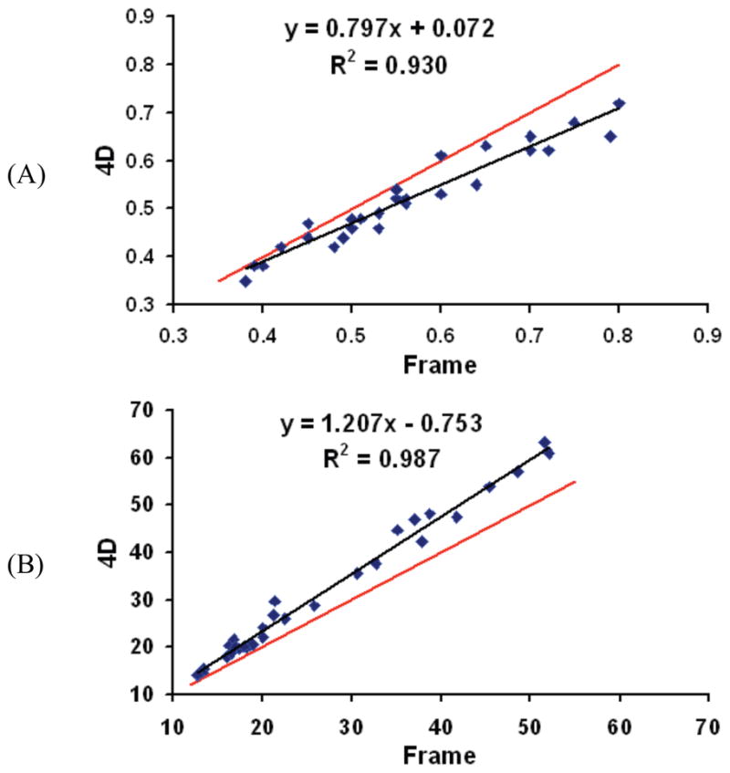
Fig. 1 shows ten typical regional values of three subjects created by 4D and frame method after 2 iterations, which were obtained from a standard template of regions applied based on MR-to-PET registration. There are consistent differences between 4D and frame methods. For K₁, 4D values are lower (mean percent difference is 10%). For V_T, 4D values are higher (mean percent difference is 16%). Some of the potential reasons for these differences are as follows:

Fig. 1.

Ten typical regional values of three subjects for frame and 4D methods. Black line is regression line and red line is identity line (A): K₁, (B): V_T

1) Resolution

Due to the intrinsic properties of iterative reconstruction algorithms, the frame method may have varying resolution across different frames (time), due to dynamic changes in image contrast, which may affect the TACs and thus the TAC fitting of the second step. However, 4D requires that all data over time be consistent with the 1T model, and thus promotes uniform resolution over time.

2) Count statistics

The frame method more likely suffers statistics-induced bias because each frame employs part of whole scan data and has poorer statistics than 4D. Note, however, that in a previous evaluation of MOLAR, low count bias was not detected in human data [12].

3) Data weighting

The optimal weighting of dynamic datasets reconstructed by the frame method requires accurate noise estimates. However it is challenging to deduce these for nonlinear iterative reconstruction algorithms. Currently, a global weight based on NEC was used for TAC fitting.

4) Activity outside brain

The current implementation of 4D enforces the 1T model for all voxels, i.e., including regions outside the brain, which is most likely not true. The frame method decouples reconstruction of emission activity image and fitting of TAC, where activity outside brain does not have impact on the ultimate parametric images. Such an effect would most likely have its largest impact on the edge of the brain, and this was not seen in the 4D results

5) Approximation of motion correction in 4D

The current approximation in the motion correction aspects of 4D could have some influence, however, this is unlikely to produce a consistent bias.

6) Differences in convergence rates

The general image patterns (see below) and the regional values are similar between frame and 4D, so a large difference in convergence is not likely. However, a more thorough evaluation of convergence is important to assess whether the disagreement in values is due, to some extent, to a difference in convergence speed.

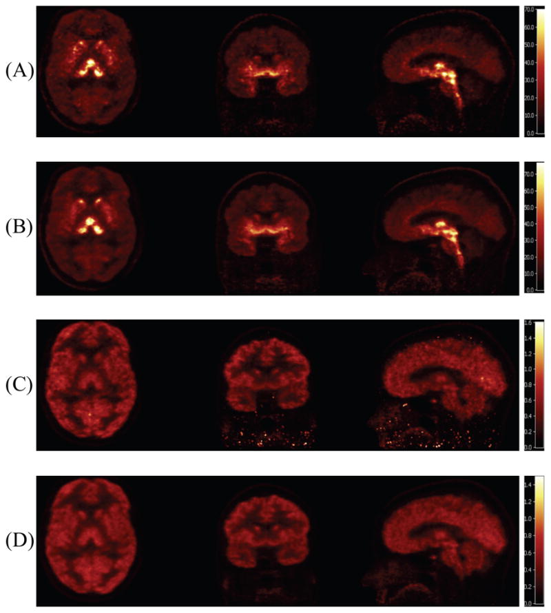
Since there are small but consistent differences between 4D and frame method results, in order to compare them fairly, different image scales were used by matching their mean values; these results are shown in Fig. 2. The distribution patterns in the two sets of images are similar with 4D showing lower noise than the frame method. This is most evident in this image on the sagittal and coronal views below the brain, where voxel data are noisier.

Fig. 2.

Parametric images reconstructed by 4D and frame methods after 2 iterations from different orientations (transverse, coronal and sagittal). (A): V_T of frame method, (B): V_T of 4D method, (C): K₁ of frame method, (D): K₁ of 4D method.

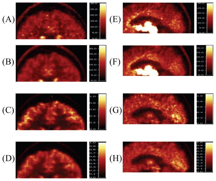
Fig. 3 shows the images zoomed in to cortex and cingulate regions. Many hot spots exist in the cortex region of frame method, with 4D appearing less noisy. This is clearest in the lack of high noise pixels in the low activity region such as white matter region and is also more noticeable in the V_T images. For the zoomed in cingulate images, 4D has clearer structure and less outliers in that region. The fact that the noise differences are most visible in the higher noise regions is consistent with previous simulation results [8].

Fig. 3.

Images zoomed into cortex (left column) and cingulate (right column) from frame and 4D methods. (A) and (E): V_T of frame method, (B) and (F): V_T of 4D method, (C) and (G): K₁ of frame method, (D) and (H): K₁ of 4D method.

V. Conclusions

In this paper, we extended the direct 4D parametric image reconstruction algorithm to include a time-continuous scatter estimate. This method was then applied to human brain data from the HRRT and we compared the resulting parametric images to those created from the conventional 2-step frame method. The initial results are encouraging, in terms of image quality and quantitative accuracy. Clearly, a much more thorough evaluation is required, in terms of the relevant accuracy and precision of the two approaches. Some of the outstanding issues include incorporation of dynamic motion correction in the model equations, evaluation with low count real data, proper modeling for regions outside brain and assessment of convergence.

References

- 1.Carson RE, Lange K. The EM parametric image reconstruction algorithm. J Am Statist Assoc. 1985;80:20–22. [Google Scholar]
- 2.Reader AJ, Sureau FC, Comtat C, Trebossen R, Buvat I. Simultaneous estimation of temporal basis functions and fully 4D PET images. IEEE Nucl Sci Symp Med Im Conf. 2006;4:2219–2223. doi: 10.1088/0031-9155/51/21/005. [DOI] [PubMed] [Google Scholar]
- 3.Kamasak ME, Bouman CA, Morris ED, Sauer K. Direct reconstruction of kinetic parameter images from dynamic PET data. IEEE Trans Med Imaging. 2005;24:636–650. doi: 10.1109/TMI.2005.845317. [DOI] [PubMed] [Google Scholar]
- 4.Wang G, Fu L, Qi J. Maximum a posteriori reconstruction of the Patlak parametric image from sinograms in dynamic PET. Phys Med Biol. 2008;53:593–604. doi: 10.1088/0031-9155/53/3/006. [DOI] [PubMed] [Google Scholar]
- 5.Wang G, Qi J. Generalized algorithms for direct reconstruction of parametric images from dynamic PET data. IEEE Trans Med Imaging. 2009;11:1717–1726. doi: 10.1109/TMI.2009.2021851. [DOI] [PMC free article] [PubMed] [Google Scholar]
- 6.Tsoumpas C, Turkheimer FE, Thielemans K. Study of direct and indirect parametric estimation methods of linear models in dynamic positron emission tomography. Med Phys. 2008;35:1299–1309. doi: 10.1118/1.2885369. [DOI] [PubMed] [Google Scholar]
- 7.Rahmim A, Zhou Y, Tang J. Direct 4D parametric image estimation in reversible tracer binding imaging. J Nucl Med. 2009;50(Supplement 2):528. [Google Scholar]
- 8.Yan J, Planeta-Wilson B, Carson RE. Direct 4D list mode parametric reconstruction for PET with a novel EM algorithm. IEEE Nucl Sci Symp Med Im Conf. 2008;3:3625–3628. doi: 10.1109/NSSMIC.2008.4774103. [DOI] [PMC free article] [PubMed] [Google Scholar]
- 9.Carson RE, Barker WC, Johnson JL. Design of a motion-compensation OSEM list-mode algorithm for resolution-recovery reconstruction for the HRRT. IEEE Nucl Sci Symp Med Im Conf. 2003;5:3281–3285. [Google Scholar]
- 10.Watson CC. New, faster, image-based scatter correction for 3D PET. IEEE Trans Nucl Sci. 2000;47:1587–1594. [Google Scholar]
- 11.Naganawa M, Planeta-Wilson B, Nabulsi N, Ropchan J, Labaree D, Neumeister A, Huang Y, Carson RE. Tracer kinetic modeling of [11C]AFM, a new PET imaging agent for the serotonin transporter. J Nucl Med. 2008;49(Supplement 1):118. [Google Scholar]
- 12.Planeta-Wilson B, Yan J, Mulnix T, Carson RE. Quantitative accuracy of HRRT listmode reconstructions: effect of low statistics. IEEE Nucl Sci Symp Med Im Conf. 2008:5121–5124. doi: 10.1109/NSSMIC.2008.4774388. [DOI] [PMC free article] [PubMed] [Google Scholar]