Radiation doses in cone-beam breast computed tomography: A Monte Carlo simulation study

Abstract

Purpose: In this article, we describe a method to estimate the spatial dose variation, average dose and mean glandular dose (MGD) for a real breast using Monte Carlo simulation based on cone beam breast computed tomography (CBBCT) images. We present and discuss the dose estimation results for 19 mastectomy breast specimens, 4 homogeneous breast models, 6 ellipsoidal phantoms, and 6 cylindrical phantoms.

Methods: To validate the Monte Carlo method for dose estimation in CBBCT, we compared the Monte Carlo dose estimates with the thermoluminescent dosimeter measurements at various radial positions in two polycarbonate cylinders (11- and 15-cm in diameter). Cone-beam computed tomography (CBCT) images of 19 mastectomy breast specimens, obtained with a bench-top experimental scanner, were segmented and used to construct 19 structured breast models. Monte Carlo simulation of CBBCT with these models was performed and used to estimate the point doses, average doses, and mean glandular doses for unit open air exposure at the iso-center. Mass based glandularity values were computed and used to investigate their effects on the average doses as well as the mean glandular doses. Average doses for 4 homogeneous breast models were estimated and compared to those of the corresponding structured breast models to investigate the effect of tissue structures. Average doses for ellipsoidal and cylindrical digital phantoms of identical diameter and height were also estimated for various glandularity values and compared with those for the structured breast models.

Results: The absorbed dose maps for structured breast models show that doses in the glandular tissue were higher than those in the nearby adipose tissue. Estimated average doses for the homogeneous breast models were almost identical to those for the structured breast models(p=1). Normalized average doses estimated for the ellipsoidal phantoms were similar to those for the structured breast models (root mean square (rms) percentage difference=1.7%;p=0.01), whereas those for the cylindrical phantoms were significantly lower (rms percentage difference=7.7%;p<0.01). Normalized MGDs were found to decrease with increasing glandularity.

Conclusions: Our results indicate that it is sufficient to use homogeneous breast models derived from CBCT generated structured breast models to estimate the average dose. This investigation also shows that ellipsoidal digital phantoms of similar dimensions (diameter and height) and glandularity to actual breasts may be used to represent a real breast to estimate the average breast dose with Monte Carlo simulation. We have also successfully demonstrated the use of structured breast models to estimate the true MGDs and shown that the normalized MGDs decreased with the glandularity as previously reported by other researchers for CBBCT or mammography.

INTRODUCTION

Mammography is widely used in the United States for routine screening of women over 40 years old for breast cancer.¹ However, mammography suffers from the overlapping of soft tissue masses and calcifications with background tissue structures on the 2D image. To solve the problem of overlapping tissue, many efforts have been made to develop techniques that produce 3D images, including mainly tomosynthesis and cone-beam breast computed tomography (CBBCT). With tomosynthesis a small number of limited angle projections are used to reconstruct pseudo-3D images. With CBBCT the patient would lie prone on a table with one breast hanging downward through an opening and scanned by an x-ray tube and detector to produce true 3D images. A great advantage of tomosynthesis is that it can be implemented by modifying a conventional digital mammography system.^{2, 3} However, tomosynthesis suffers from poor resolution along the direction of breast compression and artifacts generated from off focal plane objects. CBBCT, in contrast, provides true 3D images, which may provide more accurate and detailed information about tissue structures, lesions, and calcifications in breasts.^{4, 5, 6, 7, 8, 9, 10, 11, 12}

To realize the potential of CBBCT for true 3D breast imaging, the techniques and applications of CBBCT have been actively developed and investigated. These efforts have included feasibility studies, design and construction of prototype systems, development and investigation of new techniques, assessment of image quality, clinical evaluation, and estimation or measurement of doses.^{5, 6, 7, 8, 9, 10} It has been demonstrated with phantoms, mastectomy breast specimens, and patient study that CBBCT can be used to generate true 3D breast images with superior contrast of tissue structures and large lesions (soft tissue masses and large calcifications). Due to the limited spatial resolution, large pixel size of the detector and low exposure level used, CBBCT has yet to be improved in order to image smaller calcifications which are routinely imaged in mammography. Several prototypes have been constructed and used in clinical evaluations to demonstrate and investigate their potential use for screening and diagnosis of breast cancers. Recently clinical research showed that with the injection of contrast agent, it is likely that the compromised microcalcification detection performance of breast CT relative to mammography will become superior to mammography performance.¹³ Breast CT was significantly better than mammography for visualization of masses.^{14, 15, 16}

Despite the potential advantages of CBBCT, it is crucial to consider the radiation risk in using CBBCT for breast cancer screening and diagnosis. According to the American College of Radiology, for a 4.2-cm-thick compressed breast with 50% glandularity or breast density (both defined as the ratio of glandular tissue mass to the total breast mass), the maximum allowed mean glandular dose (MGD) is 6 mGy for two view mammograms.¹⁷ Following this practice, many researchers have considered that the maximum dose at the isocenter should be limited to≤6 mGy.¹⁸ Because of the multiexposure geometry of CBBCT, accurate dose control is very important, and thus the estimation of breast dose for CBBCT has wide interest.^{19, 20, 21, 22}

Two methods are often used to estimate radiation dose: physical measurement and Monte Carlo simulation. For physical measurement, thermoluminescent dosimeters (TLDs) and ion chambers are widely used.²¹ Both are portable and can be placed inside specially designed tissue-equivalent phantoms to estimate radiation doses at various locations in the breast phantoms. However, because the measurements could be performed at a limited number of sampling positions, average breast doses could not be directly measured.

To overcome the limitations of experimental measurements, Monte Carlo simulation has been widely used to mimic the CBBCT system and to estimate the 3D dose variation for various breast sizes, shapes, and compositions. Boone et al. used the SIERRA Monte Carlo code to estimate normalized glandular dose in CT (DgN_CT) for CBBCT by using cylindrical digital phantoms of various diameters and tissue compositions for 30–100 kVp polyenergetic x-rays.²⁰ Glick et al. employed the GEANT3 Monte Carlo code to estimate the doses in cylindrical breast phantoms for various combinations of acquisition geometry, kVp, pixel size, and scintillator thickness.²¹ To better mimic an uncompressed, pendant breast, Ning et al. used three half-ellipsoidal digital phantoms of different sizes to estimate and use mean absorbed exposure-to-dose conversion factor (D_gN) to convert the entrance exposure in a single projection view to the average dose for full scan.⁷

Average doses and spatial dose variation have been estimated and investigated for simple geometric or structured breast phantoms for various mammography techniques.^{23, 24, 25} They have also been estimated and investigated for CBBCT.¹⁹ However, the average dose and spatial dose variation have not been studied for realistic breasts in CBBCT. In this study, we constructed 19 structured breast models derived from segmented CBBCT images of mastectomy specimens to better mimic uncompressed, pendant breasts. We estimated spatial dose variation, average doses, and MGDs by Monte Carlo simulations of CBBCT. We compared the average doses for structured breast models with those for simplified, homogeneous breast models: breast-shaped, cylindrical, and half-ellipsoidal (hereafter referred to as ellipsoidal) phantoms with various breast densities.

METHODS AND MATERIALS

CBBCT system

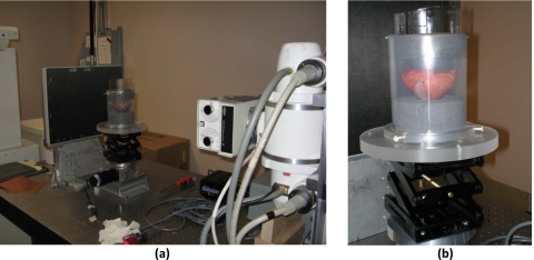
An experimental CBBCT system with a flat-panel digital detector was built on an optical bench in our laboratory [Fig. 1a].²⁶ This system consisted of three components: an x-ray unit, an amorphous silicon∕cesium iodide (a-Si:H∕CsI) flat-panel detector, and a step motor-driven rotary table. The x-ray unit consisted of an x-ray generator (Indico 100 SP, Communications & Power Industries, Georgetown, Canada) coupled to an x-ray tube (G1592BI∕B180, Varian Medical Systems, Salt Lake City, UT) with a nominal focal spot size of 0.6 or 1.2 mm. The flat-panel detector (PaxScan 4030CB, Varian Medical Systems) had a 2048×1536 array of194-μm pixels, resulting in a 40×30 cm² active image area. The phantom or specimen was placed on the rotary table, which was driven by a stepping motor (B4872TS, Velmex, Bloomfield, NY) and rotated during the scan to simulate CBBCT with a rotating gantry. The distances from the x-ray source to the isocenter and to the detector were 75 cm and 100 cm, respectively, resulting in a magnification of 1.33. (Fig. 2) Notice that this acquisition geometry was duplicated in Monte Carlo simulation.

Figure 1.

(a) A bench-top experimental CBCT system with (b) a breast specimen placed on the rotating table.

Figure 2.

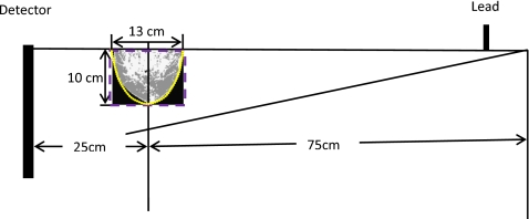
Geometry for Monte Carlo simulations. Structured breast models (grayscale), ellipsoidal phantoms (dotted contour), and cylindrical phantoms (dashed contour) were irradiated. The voxel size was 1.305×1.305×1.305 mm³ for the structured breast models and 1×1×1 mm³ for the geometric phantoms. A 2-mm-thick lead plate was used to form a half-cone-beam. The source-to-object distance was 75 cm. To simplify the Monte Carlo simulation, we assumed that x-rays were generated from a point source.

Digital breast models and phantoms

Structured breast models

To compute and study spatial dose variation and average dose for actual breasts, we used CBCT images of 19 mastectomy breast specimens to construct 19 different digital structured breast models for the Monte Carlo simulation. These images were acquired with breasts removed in the mastectomy operations for patients recruited and consented under an IRB approved protocol (LAB05–0588). Each specimen was placed in a bowl shaped holder on the rotary table for CBCT imaging. During the scan it was rotated for 360° while 300 projection images were acquired with x-rays generated at 80 kVp with a half value layer of 4.08 mm aluminum. Based on mammography performed before the mastectomy, 13 of these breasts were categorized as “heterogeneously dense,” and the rest as “scattered fibroglandular.”

The CBBCT images were first corrected to remove cupping artifacts and then filtered to reduce the noise level. The processed images were then segmented using the threshold method to separate the breast into glandular and adipose tissue regions. Each CBBCT image set consisted of 600–1200 slices of 900×900 images with a voxel size of0.145×0.145×0.145 mm³. To achieve reasonable simulation speed, we binned the images into 100×100×(75–84) matrix sizes with a voxel size of1.305×1.305×1.305 mm³. To compute the attenuation coefficients for Monte Carlo simulation, the elemental composition and density of glandular tissue were adopted from a report by Hammerstein et al.,²⁷ while those of adipose tissue were adopted from a more recent report by the National Institute of Standards and Technology (NIST).²⁸

The glandularity was computed as the ratio of the glandular tissue mass to the total breast mass. The former was computed as the product of number of glandular tissue voxels, the voxel volume, and the density of glandular tissue. The adipose tissue mass was computed in a similar way. The total breast mass was computed as the sum of the glandular tissue mass and the adipose tissue mass. For the 19 breasts studied, the computed breast density was found to range from 18% to 58%.

Homogeneous breast models

To investigate the effects of tissue structures on the average dose, we selected four structured breast models with a range of different glandularities (33%, 36%, 43%, and 48%) and replaced the tissue structures with homogeneous tissue with identical glandularities. These models were referred to as the homogeneous breast models in this paper.

Ellipsoidal and cylindrical phantoms

To investigate the accuracy in using simple, homogeneous geometric phantoms to represent breasts in Monte Carlo simulation and dose estimation, we constructed a series of ellipsoidal and cylindrical digital phantoms. To match the dimensions of the structured breast models used, both the ellipsoidal and cylindrical phantoms were created with a diameter of 13 cm and a height of 10 cm. All the geometric phantoms had a voxel size of1×1×1 mm³, and the glandularity values used were 0%, 20%, 40%, 60%, 80%, and 100%. In Fig. 2, the contours of these two phantoms are drawn along with a structured breast model as aligned with the isocenter in the acquisition layout.

Phantoms for validation

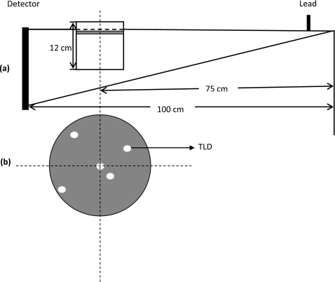
To validate dose estimates using Monte Carlo method, we constructed two polycarbonate cylinder phantoms, one with a diameter of 11 cm and the other with a diameter of 15 cm and both with a height of 12 cm. (Fig. 3) 5-mm-diameter holes were opened at 0, 0.73, 1.76, 3.0, and 5.1 cm from the central axis for the small phantom and 0, 0.73, 1.76, 3.0, 5.1, and 7.1 cm from the central axis for the large phantom to allow the TLDs to be inserted and positioned at 1.25 cm below the top surface for dose measurement. (Fig. 3) Two digital phantoms, both with three different voxel sizes of1×1×10, 1×1×5, and 1×1×115 mm³ from top to bottom, were created to mimic these two cylindrical phantoms and used for Monte Carlo simulation and dose estimation.

Figure 3.

Acquisition geometry for TLD measurements and Monte Carlo simulations for validation. Two 12-cm-high polycarbonate cylinders, one 11 cm and the other 15 cm in diameter, were imaged. The voxel size was 1×1×5 mm³ for the 5-mm-thick layer containing the TLDs, 1×1×10 mm³for the 10 mm thick layer above the TLDs and 1×1×115 mm³ for 115 mm layer below the TLDs. (Upper gray area) A 2-mm-thick lead plate was used to form a half-cone-beam. The source-to-object distance was 75 cm. To simplify the Monte Carlo simulation, we assumed that x-rays were generated from a point source. The positioning of TLDs are illustrated in bellow the geometry.

Monte Carlo simulation

We used the BEAMNRC∕EGSNRC code²⁹ to simulate 10⁸ primary photons emitted from the x-ray source point. The photons were generated at 80 kVp with a 12° tungsten target and filtered by 5-mm-thick aluminum, resulting in a half-value layer (HVL) of 4.08 mm aluminum which matched the measured HVL for the x-ray beam used in our validation measurement. The x-ray spectrum was computed using a previously published program, SRS-78,³⁰ for use with the simulation. Since half-cone-beam is usually used in CBBCT, a 2-mm-thick lead collimator was incorporated in BEAMNRC to collimate the x-rays into a half-cone-beam which consisted of about 5×10⁷ photons at the exit of the collimator (Fig. 2). The energies, positions, and directions of these photons were recorded as a data file, referred to as the phase space file in the code, and used for subsequent image simulation and dose estimation. To verify the intensity variation of the half-cone-beam generated, we used the BEAMDP (Ref. ³¹) (BEAM data processor) code to derive the spatial variation of the photon fluence at the exit of the collimator.

The phase space file was used with the DOSXYZNRC code³² to randomly generate 10⁹ incident photons to simulate x-ray exposure to our digital breast models or phantoms with 300 projection views evenly spread over 360°. The cutoff energies for photon transport and electron transport were set at 1 and 512 keV, respectively, in all components of the codes. All attenuation data were produced with the PEGS4 code as required by EGSNRC code. The included interactions were bremsstrahlung production, Coulomb scattering, Compton scattering, Rayleigh scattering, and the photoelectric effect. The energy deposited by the photons was tallied for each voxel to estimate the dose on a voxel-by-voxel basis. The doses were then averaged over the entire breast volume to compute the average dose $\overline{D}$ as follows:

$$\overline{D}=\frac{{\sum }_{i=1}^{N}D\left(i\right)\times V\times \rho \left(i\right)}{{\sum }_{i=1}^{N}V\times \rho \left(i\right)},$$ (1)

where N is the total number of voxels, D(i)is the dose for the ith voxel, Vis the volume of a voxel, and ρ(i) is the density of the ith voxel. For structured breast models, the MGD was also computed by averaging the doses in all glandular tissue voxels. For normalization, the free air kerma was estimated at the isocenter with Monte Carlo simulation using the same number of photons. All dose estimates were normalized by the free air kerma and presented as dose (mGy) per unit air kerma (mGy) for comparison.

Validation with TLD measurements

To validate our Monte Carlo method for simulating doses, TLDs of lithium fluoride doped with magnesium and titanium (LiF:Mg,Ti) were used to measure doses at selected locations in the two polycarbonate cylindrical phantoms and compared them with the results from Monte Carlo simulation. To ensure the x-ray beam quality was kept the same for the comparison, the HVL was measured to be 4.08 mm aluminum with an ion chamber (10X5–6, Radcal, Monrovia, CA) and type 1100 aluminum sheets and used to determine the filtration of the x-ray spectrum for Monte Carlo simulation. For TLD dose measurements, x-rays were collimated to form a half-cone-beam. With the measurement, each cylindrical polycarbonate phantom was positioned at the isocenter with its top at 8 mm above the upper edge of the half-cone-beam (Fig. 3). The phantom was rotated for 360° during the exposure to simulate CBBCT with a rotating source–detector gantry. 33 msec pulsed exposures were made with tube currents of 25 and 29 mA for the small and large phantoms, respectively.

After the exposures, signals were read out using a TLD reader (Harshaw 3500, Harshaw-Bicron, Newbury, OH). For calibration, signals obtained at various exposure levels were plotted as a function of the absorbed dose calculated from the exposure to obtain a calibration curve. The absorbed doses in this study were then computed using the calibration curve and plotted as a function of the radial distance from the central axis of the phantoms.

For normalization, the free air kerma measured with an ion chamber were 3.2, 7.1, 15.6, 32.4, and 49.2 mGy at the isocenter for 30, 60, 120, 240, and 360 mAs, respectively. As with Monte Carlo dose estimation, all dose measurements were normalized by the free air kerma and presented as dose (mGy) per unit free air kerma (mGy).

Comparison of dose values

All dose estimates or measurements were normalized by the free air kerma at the isocenter before being compared to each other. However, for simplicity of presentation, they are sometimes referred to as the doses only hereafter in this paper. To compare the Monte Carlo estimates and TLD measurements, the percentage difference was individually given for each pair of corresponding estimate and measurement. The root mean square (rms) percentage difference was computed for the two groups of data. Because the data were not normally distributed, the Wilcoxon Signed Rank test was used instead of the paired t-test to compute the p-value. Linear regression was also performed to quantify and study the correlation between the two groups of data. The linear fit values was forced to go through the origin as both the Monte Carlo estimate and TLD measurement would extrapolate to zero with zero x-ray exposure. Similar analysis was performed to compare the average doses of the ellipsoidal and cylindrical phantoms with those of the structured breast models.

RESULTS

Validation of Monte Carlo package

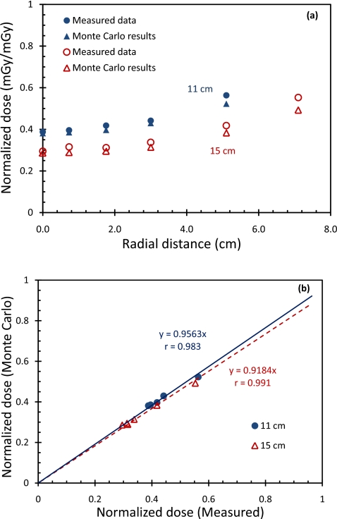
In Fig. 4a, normalized TLD measurements and Monte Carlo estimates are plotted as a function of the radial position for both small and large polycarbonate cylindrical phantoms. The TLD measurements were found to be consistently higher than the Monte Carlo estimates. The percentage differences between the TLD measurements and the Monte Carlo estimate were found to be 1.7%–7.2% (rms percentage difference=4.3%;p=0.06) and 3.0%–10.9% (rms percentage difference=7.5%;p=0.03) for the small and large phantoms, respectively. Following the linear regression, the Monte Carlo dose estimates are plotted against the corresponding normalized TLD dose measurements. The correlation coefficients were calculated to be 0.983 and 0.991 for the small and large phantoms, respectively. The slopes of the fittings were calculated to be 0.956 and 0.918 for the small and large phantoms, respectively.

Figure 4.

(a) Comparison of normalized dose from experimental measurements with Monte Carlo estimates for 11-cm-diam (solid symbol) and 15-cm-diam (hollow symbol) cylindrical phantoms. (b) The Monte Carlo derived doses are plotted against the corresponding TLD measurements and correlation coefficients were given for small and large cylindrical phantoms, respectively.

Estimated dose variation for structured breast models

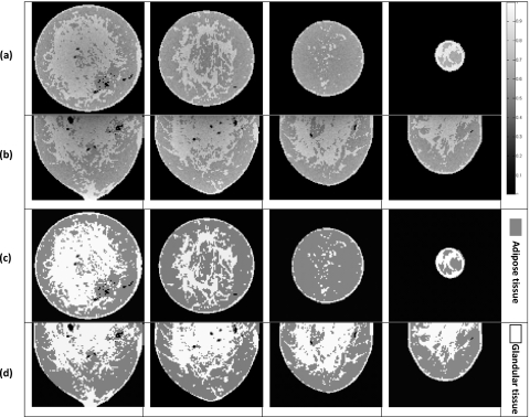
A set of segmented CBBCT images and the corresponding spatial dose variations are shown in Fig. 5. The absorbed dose maps closely mirrored the tissue structures in the segmented CBBCT images, and the estimated doses were higher in the glandular tissue than in the neighboring adipose tissue.

Figure 5.

Monte Carlo dose estimates for structured breast models. (a) Spatial dose variation for coronal slices (6.5, 26.1, 45.7, and 65.3 mm from the chest wall, respectively) and (c) the corresponding structures on CBBCT images. (b) Spatial dose variation for sagittal slices (6.5, 19.6, 32.6, and 45.7 mm from the central axis, respectively) and (d) the corresponding structures on CBBCT images. Dose values are plotted using a gray scale.

Comparison of average doses for structured and homogeneous breast models

Monte Carlo simulation was performed for four homogeneous breast models derived from four structured breast models with glandularities of 33%, 36%, 43%, and 48%. The normalized average doses were estimated to be 0.59, 0.59, 0.61, and 0.60 mGy∕mGy, respectively. There was little difference (p=1.000) between these values and those for the structured breast models.

Comparison of estimated doses for structured breast models, ellipsoidal phantoms, and cylindrical phantoms

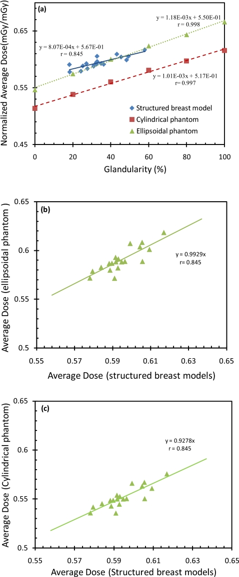
In Fig. 6a, the normalized average doses are plotted as a function of the glandularity for the structured breast models and the ellipsoidal and cylindrical phantoms. The plots show that dose estimates with the ellipsoidal phantoms were close to those with the structured breast models. The dose estimates with the cylindrical phantoms, on the other hand, were found to be consistently lower. Because the ellipsoidal and cylindrical phantoms studied had different glandularities (0% 20%, 40%, 60% 80%, and 100%) from those of the structured breast models (18%–58%), a quantitative comparison could not be directly performed. Linear equations relating the normalized average doses to the glandularity were obtained and then compared with each other (Fig. 6b, 6c). The equations for the ellipsoidal and cylindrical phantoms were also used to compute the normalized average doses for the 19 glandularity values of the structured breast models. The doses for the ellipsoidal phantom were found to agree well with those obtained with the structured breast models (rms percentage difference=1.7%;p=0.01), while those for the cylindrical phantoms significantly lower (rms percentage difference=7.7%;p<0.01). In Figs. 6b, 6c, the dose estimates for the two phantoms were plotted separately against the corresponding dose estimates for the structured breast models. Linear regressions resulted in a correlation coefficient of 0.845 for both phantoms, a slope of 0.993 for the ellipsoidal phantom and 0.928 for the cylindrical phantom.

Figure 6.

(a) Normalized average dose versus glandularity. Normalized average doses were calculated for structured breast models, cylindrical phantoms, and ellipsoidal phantoms, respectively. The rms percentage difference between structured breast models and ellipsoidal phantoms is 1.7% and between structured breast models and cylindrical phantoms is 7.7%. (b) The Monte Carlo derived average doses for ellipsoidal phantoms are plotted against those for structured breast models. (c) The Monte Carlo derived average doses for cylindrical phantoms are plotted against those for structured breast models.

Mean glandular dose for structured breast models

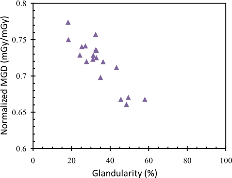
In Fig. 7, normalized MGD is plotted as a function of glandularity for our 19 structured breast models. Normalized MGD was found to decrease with increasing glandularity. This result is similar to the previously reported findings on the variation of MGD with glandularity in mammography.

Figure 7.

Normalized MGD for 19 structured breast models.

DISCUSSION

In this study, we used Monte Carlo simulation to estimate and compare doses for 19 structured breast models, 4 homogeneous breast models, 6 ellipsoidal phantoms, and 6 cylindrical phantoms. Although structured phantoms or models have been previously used to estimate doses^{23, 24, 25} or to investigate image quality^{33, 34} in various digital mammography techniques, no structured models or phantoms have been used to estimate doses in CBBCT. Furthermore, our structured breast models were derived from segmented images of mastectomy breast specimens and contained realistic breast tissue structures with both adipose and glandular tissues. In addition to using these models to estimate the average doses, we also used them to estimate the true MGDs, which cannot be accurately estimated with the commonly used homogeneous phantoms.

To validate the Monte Carlo model, we compared normalized TLD measurements with normalized Monte Carlo estimates at various locations inside two cylindrical phantoms. The Monte Carlo estimates were slightly lower than the TLD measurements with rms percentage differences of 4.3% and 7.5% for the small and large phantoms, respectively. There are several possible causes for this discrepancy. First, although we tried to match the locations and sampling volumes for Monte Carlo dose estimation with those for TLD measurements as accurately as possible, there could still be some deviation. Second, although the x-ray spectrum used for Monte Carlo simulation was selected to result in the same HVL as for the x-ray spectrum used in the TLD measurements, this does not guarantee that the two spectra were identical. Third, the heel effect was not modeled in our simulation for simplicity. This may have resulted in differences in both photon fluences and spectra between Monte Carlo simulation and TLD measurement.

Results with our structured breast models show that the glandular tissue voxels had higher estimated doses than the neighboring adipose tissue voxels and the absorbed dose map closely mirrored the pattern of tissue structures in the segmented CBBCT images. Both results were expected because the energy absorption coefficients of glandular tissue are known to be higher than those of adipose tissue.²⁸

We also investigated the dependence of the average breast dose on the shape, dimensions, and tissue structures of the breasts. Comparison of the linear fit values shows that the average doses estimated for ellipsoidal and cylindrical phantoms correlated well (r=0.998and 0.997) and increased linearly with the glandularity (Fig. 6). The average doses for the 19 structured breast models could also be fitted to a linear relationship with the glandularity but with poorer correlation (r=0.845) as shown by the fluctuations around the fitted line. Comparing the dose estimates for the 19 glandularity values of the structured breast models, the ellipsoidal phantoms resulted in estimates closer to those for the structured breast models (rms percentage difference=1.7%;p=0.01), while that the cylindrical phantoms resulted in significantly lower estimates (rms percentage difference=7.7%;p<0.01). This is also reflected by the different slopes of the plots in Figs. 6b, 6c. This finding indicates that an ellipsoidal phantom of similar dimensions (diameter and height) and identical glandularity may be used to estimate the average dose of a real breast with much better accuracy than the cylindrical phantoms.

We also found that dose estimates for structured breast models fluctuated significantly from their linear fit values while those for ellipsoidal or cylindrical phantoms had little fluctuations from theirs. The fluctuation of dose estimates for the structured breast models could be due to the variation of the breast dimensions, shape, or tissue structures from breast to breast. To investigate whether the tissue structures would influence the estimation of average dose, we computed and compared doses for four structured breast models and four homogenous breast models which were derived from them. No significant difference in estimated doses was found between these two groups of models. (p=1orp⪢0.05). Thus, the fluctuations of the estimated doses for the structured breast models from their linear fit values were probably due to the variation of the breast shape and dimensions rather than differences in tissue structures. In the cases of ellipsoidal and cylindrical phantoms, the doses were estimated for phantoms of the same dimensions and shape but varying glandularity, thus the estimates fluctuated little from their linear fit values. The fluctuation of the dose estimates for the structured breast models from their linear fit values indicates that although an ellipsoidal phantom with similar dimensions and identical glandularity is a good candidate for estimating the average dose with Monte Carlo simulation, it may be subject to small deviation due to the slight differences in the shape and dimensions between the phantom and the breast it represents.

We also estimated the MGDs for structured breast models. Figure 7 shows that the normalized MGD decreased with the glandularity. Table 1 also shows normalized MGDs as for various parameters. This is similar to the previously reported relationships of the normalized MGD and the glandularity in mammography (D_gN) and between that in CBBCT(DgN_CT), estimated with other methods.^{35, 36} It should be noted that although the MGD decreased with the glandularity, the total radiation energy absorbed by the glandular tissue, which has been suggested to be more linked to the cancer risk, actually increased because the total glandular tissue mass increased at a much faster rate with the glandularity. It should also be noted that the estimation of the MGD through the use of Monte Carlo simulation with a structured breast model derived from the CBCT images allowed doses for glandular tissue voxels and thus the MGD to be directly estimated as the voxels of the model contain either pure glandular tissue or pure adipose tissue. In contrast, the use of a homogeneous model or phantom would require the conversion of doses estimated for mixed (partially glandular and partially adipose) tissue into those for pure glandular tissue. Point-by-point estimation of the factors required for such conversion could be tedious and difficult if not impossible.²⁴

Table 1.

Normalized MGDs (mGy∕mGy) of structured breasts for different glandularities and sizes.

Glandularity (%)	Size (cm3)
	13.05×13.05×9.8	13.05×13.05×11.0
18.2	1.01
18.4	0.98
24.3	0.95
25.3	0.96
27.2	0.97
27.7		0.94
31.0	0.94
31.3	0.95
32.4	0.99
32.5	0.96
32.8	0.96	0.94
35.0	0.91
36.3	0.94
43.3	0.93
45.5	0.87
48.4	0.86
49.4		0.87
57.9		0.87

One shortcoming of this study is that since the skin is usually left attached to the chest for sealing the wound in a mastectomy operation, it is absent in our structured breast models. This may result in a slightly inaccurate representation of real breasts. This problem can be resolved in the future by using CBBCT images of normal patients and those obtained prior to the mastectomy operation. Another shortcoming is the lack of heel effect in our modeling of the x-ray source. These shortcomings will be investigated and resolved in our future studies.

CONCLUSIONS

In this study, we used Monte Carlo simulation to estimate and compare normalized average doses for 19 structured breast models, 4 homogeneous breast models, 6 ellipsoidal phantoms, and 6 cylindrical phantoms. Structured breast models derived from real breasts have been used to study the spatial dose variation and average dose over the entire breast in CBBCT therefore true MGD can be studied. Results with our structured breast models show that the glandular tissue voxels had higher estimated doses than the neighboring adipose tissue voxels and the absorbed dose map closely mirrored the pattern of tissue structures in the segmented CBBCT images. The normalized average doses for the structured breast models were found to increase with the glandularity. On the other hand, the normalized MGDs for these models were found to decrease with the glandularity. Results with four homogeneous breast models show that the presence of complex tissue structures had little effect on the estimation of normalized average dose. Normalized average doses estimated for the ellipsoidal phantoms and those for the cylindrical phantoms were both found to increase linearly with the glandularity with little fluctuations. Comparison of the linear fit values shows that doses estimated for the ellipsoidal phantoms were much closer to those for structured breast models while those for the cylindrical phantoms were significantly lower. Thus, an ellipsoidal phantom of similar dimensions (diameter and height) and identical glandularity may be used to estimate the average breast dose with Monte Carlo simulation.

References

- American Cancer Society, Cancer Facts and Figures 2008 (2008).
- Niklason L. T. et al. , “Digital tomosynthesis in breast imaging,” Radiology 205, 399–406 (1997). [DOI] [PubMed] [Google Scholar]
- Glick S. J. and Gong X., “Optimal spectra for indirect detector breast tomosynthesis,” Proc. SPIE 6142, 61421L (2006). 10.1117/12.649547 [DOI] [Google Scholar]
- Madhav P., Crotty D. J., McKinley R. L., and Tornai M. P., “Evaluation of tilted cone-beam CT orbits in the development of a dedicated hybrid mammotomograph,” Phys. Med. Biol. 54, 3659–3676 (2009). 10.1088/0031-9155/54/12/004 [DOI] [PMC free article] [PubMed] [Google Scholar]
- Glick S. J., “Breast CT,” Annu. Rev. Biomed. Eng. 9, 501–526 (2007). 10.1146/annurev.bioeng.9.060906.151924 [DOI] [PubMed] [Google Scholar]
- Boone J. M., Nelson T. R., Lindfors K. K., and Seibert J. A., “Dedicated breast CT: Radiation dose and image quality evaluation,” Radiology 221, 657–667 (2001). 10.1148/radiol.2213010334 [DOI] [PubMed] [Google Scholar]
- Chen B. and Ning R., “Cone-beam volume CT breast imaging: Feasibility study,” Med. Phys. 29, 755–770 (2002). 10.1118/1.1461843 [DOI] [PubMed] [Google Scholar]
- Gong X., Vedula A. A., and Glick S. J., “Microcalcification detection using cone-beam CT mammography with a flat-panel imager,” Phys. Med. Biol. 49, 2183–2195 (2004). 10.1088/0031-9155/49/11/005 [DOI] [PubMed] [Google Scholar]
- Ning R. et al. , “Evaluation of flat panel detector-based cone beam CT breast imaging with different sizes of breast phantoms,” Proc. SPIE 5745, 626–636 (2005). 10.1117/12.596127 [DOI] [Google Scholar]
- Yang W. T. et al. , “Dedicated cone-beam breast CT: Feasibility study with surgical mastectomy specimens,” AJR, Am. J. Roentgenol. 189, 1312–1315 (2007). 10.2214/AJR.07.2403 [DOI] [PMC free article] [PubMed] [Google Scholar]
- Chen L. et al. , “Spatial resolution properties in cone beam CT: A simulation study,” Med. Phys. 35, 724–734 (2008). 10.1118/1.2829867 [DOI] [PMC free article] [PubMed] [Google Scholar]
- Glick S., Vedantham S., and Karellas A., “Investigation of optimal kVp settings for CT mammography using a flat panel detector,” Proc. SPIE 4682, 392–402 (2002). 10.1117/12.465581 [DOI] [Google Scholar]
- Prionas N. D. et al. , “Contrast-enhanced dedicated breast CT: Initial clinical experience,” Radiology 256, 714–723 (2010). 10.1148/radiol.10092311 [DOI] [PMC free article] [PubMed] [Google Scholar]
- Lindfors K. K. et al. , “Dedicated breast CT: Initial clinical experience,” Radiology 246, 725–733 (2008). 10.1148/radiol.2463070410 [DOI] [PMC free article] [PubMed] [Google Scholar]
- O’Connell A. et al. , “Cone-beam CT for breast imaging: Radiation dose, breast coverage, and image quality,” AJR, Am. J. Roentgenol. 195, 496–509 (2010). 10.2214/AJR.08.1017 [DOI] [PubMed] [Google Scholar]
- Boone J. M. et al. , “An x-ray computed tomography∕positron emission tomography system designed specifically for breast imaging,” Technol. Cancer Res. Treat. 9, 29–43 (2010). [DOI] [PMC free article] [PubMed] [Google Scholar]
- Feig S. A., “American College of Radiology guidelines for breast cancer screening,” AJR, Am. J. Roentgenol. 171, 29–33 (1998). [DOI] [PubMed] [Google Scholar]
- Basset L.et al. , ACR Practice Guideline for the Performance of Screening and Diagnostic Mammography (American College of Radiology, Reston, VA, 2008). [Google Scholar]
- Sechopoulos I. et al. , “Monte Carlo and phantom study of the radiation dose to the body from dedicated CT of the breast,” Radiology 247, 98–105 (2008). 10.1148/radiol.2471071080 [DOI] [PMC free article] [PubMed] [Google Scholar]
- Boone J. M., Shan N., and Nelson T. R., “A comprehensive analysis of DgNCT coefficients for pendant-geometry cone-beam breast computed tomography,” Med. Phys. 31, 226–235 (2004). 10.1118/1.1636571 [DOI] [PubMed] [Google Scholar]
- Thacker S. C. and Glick S. J., “Normalized glandular dose (DgN) coefficients for flat-plane CT breast imaging,” Phys. Med. Biol. 49, 5433–5444 (2004). 10.1088/0031-9155/49/24/003 [DOI] [PubMed] [Google Scholar]
- Russo P. et al. , “Dose distribution in cone-beam breast computed tomography: An experimental phantom study,” IEEE Trans. Nucl. Sci. 57, 366–374 (2010). 10.1109/TNS.2009.2036848 [DOI] [Google Scholar]
- Dance D. R. et al. , “Breast dosimetry using high-resolution voxel phantoms,” Radiat. Prot. Dosim. 114, 359–363 (2005). 10.1093/rpd/nch510 [DOI] [PubMed] [Google Scholar]
- Bliznakova K., Kolitsi Z., and Pallikarakis N., “Dual-energy mammography: Simulation studies,” Phys. Med. Biol. 51, 4497–4515 (2006). 10.1088/0031-9155/51/18/004 [DOI] [PubMed] [Google Scholar]
- Ma A. K. W., Gunn S., and Darambara D. G., “Introducing DeBRa: A detailed breast model for radiological studies,” Phys. Med. Biol. 54, 4533–4545 (2009). 10.1088/0031-9155/54/14/010 [DOI] [PubMed] [Google Scholar]
- Lai C. -J. et al. , “Visibility of microcalcification in cone beam breast CT: Effects of x-ray tube voltage and radiation dose,” Med. Phys. 34, 2995–3004 (2007). 10.1118/1.2745921 [DOI] [PMC free article] [PubMed] [Google Scholar]
- Hammerstein G. R. et al. , “Absorbed radiation-dose in mammography,” Radiology 130, 485–491 (1979). [DOI] [PubMed] [Google Scholar]
- Hubbell J. H. and Seltzer S. M., “Tables of x-ray mass attenuation coefficients and mass energy-absorption coefficients from 1 keV to 20 MeV for elements Z=1 to 92 and 48 additional substances of dosimetric interest,” The National Institute of Standards and Technology (1996).
- Nelson W. R., Hirayama A., and Rogers D. W. O., The EGS4 Code System (Stanford Linear Accelerator Center, Menlo Park, CA, 1985). [Google Scholar]
- Cranley K.et al. , “Catalogue of diagnostic x-ray spectra and other data,” IPEM Report No. 78, 1997.
- Ma C. -M. and Rogers D. W. O., “BEAMDP Users Manual, NRCC Report No. PIRS-0509(C)revA, 2006.
- Walters B. R. B. and Rogers D. W. O., “DOSXYZnrc Users Manual, NRCC Report No. PIRS-794revB, 2004.
- Bakic P. R. et al. , “Mammogram synthesis using a 3D simulation. 1. Breast tissue model and image acquisition simulation,” Med. Phys. 29, 2131–2139 (2002). 10.1118/1.1501143 [DOI] [PubMed] [Google Scholar]
- Bakic P. R. et al. , “Mammogram synthesis using a 3D simulation. II. Evaluation of synthetic mammogram texture,” Med. Phys. 29, 2140–2151 (2002). 10.1118/1.1501144 [DOI] [PubMed] [Google Scholar]
- Wu X., Barnes G. T., and Tucker D. M., “Spectral dependence of glandular tissue dose in screen-film mammography,” Radiology 179, 143–148 (1991). [DOI] [PubMed] [Google Scholar]
- Wu X. et al. , “Normalized average glandular dose in molybdenum target-rhodium filter and rhodium target-rhodium filter mammography,” Radiology 193, 83–89 (1994). [DOI] [PubMed] [Google Scholar]