Bayesian ensemble methods for survival prediction in gene expression data

Abstract

Motivation: We propose a Bayesian ensemble method for survival prediction in high-dimensional gene expression data. We specify a fully Bayesian hierarchical approach based on an ensemble ‘sum-of-trees’ model and illustrate our method using three popular survival models. Our non-parametric method incorporates both additive and interaction effects between genes, which results in high predictive accuracy compared with other methods. In addition, our method provides model-free variable selection of important prognostic markers based on controlling the false discovery rates; thus providing a unified procedure to select relevant genes and predict survivor functions.

Results: We assess the performance of our method several simulated and real microarray datasets. We show that our method selects genes potentially related to the development of the disease as well as yields predictive performance that is very competitive to many other existing methods.

Availability: http://works.bepress.com/veera/1/.

Contact: veera@mdanderson.org

Supplementary Information: Supplementary data are available at Bioinformatics online.

1 INTRODUCTION

Gene expression profiling using DNA microarray technology has successfully identified molecular classes of cancer and revealed gene expression patterns that are associated with disease recurrence or prognosis of patient survival (Berchuck et al., 2005). Survival prediction is often formulated in terms of categorical outcomes (e.g. ‘poor’ versus ‘good’ prognosis), which may be useful for guiding decisions about cancer management and treatment (Ross, 2009). However, due to a large degree of heterogeneity observed within prognostic classes, prediction of time to a clinical event/occurrence may not be successful. Improved accuracy of survival prediction can be attained by relating time-to-event measures directly with gene expression profiles, which requires specific survival analysis methods that account for the presence of right censored outcomes, such as the (multivariable) Cox proportional hazards (CPH) model (Cox, 1972) and the accelerated failure time model (AFT; Klein and Moeschberger, 1997). In our context, we define the (uncensored) survival time as the dependent variable of interest representing the time to an event (such as death or recurrence), and a right censored observation is an observation that is lost to follow-up after the period of study.

In spite of their widespread use in other settings, these standard multivariable survival methods cannot be directly applied to clinical outcome prediction using gene expression data because the number of covariates (genes) under investigation is considerably larger than the number of samples (patients)—the ‘large p, small n problem’ (West, 2003). Many different strategies have been employed to solve this high dimensionality problem. For example, clustering techniques have been applied to group-correlated sets of genes, (D'haeseleer, 2005), linear combinations of covariates obtained by the partial least squares method (Nguyen and Rocke, 2002; Park et al., 2002) or the principal components of the design matrix (Li and Gui, 2004) have been used as explanatory variables in survival regression models. In addition, some authors have proposed the use of penalized versions of the CPH model, L1-penalized (Lasso regression) and L2-penalized (ridge regression) versions, for estimating parameters while simultaneously performing variable selection (Gui and Li, 2005; Park et al., 2002; Tibshirani, 1997). Similarly, Datta et al. (2007) developed penalized variants of the AFT model for fitting high-dimensional datasets. Bayesian techniques for variable selection have also been developed for Weibull and CPH models (Lee and Mallick, 2004) as well as for the AFT model (Sha et al., 2006).

Although these strategies address the high-dimensionality problem with some degree of success, they fail to incorporate complex interactions between genes because they model genes in an additive and linear manner. Ensemble methods such as bagging (Breiman, 1996), boosting (Friedman, 2001) and random forests (Breiman, 2001) are flexible alternatives for accommodating variable interactions that are more stable in high-dimensional settings (Breiman, 2001). Because ensemble methods use a linear combination of trees to fit data variations such that each tree fits part of the data, these methods have been shown to have high predictive accuracy (Lee et al., 2005). The ensemble methods were originally developed for modeling binary or continuous responses. Extensions for modeling survival data, often called survival ensembles (Hothorn et al., 2006), address the censoring problem by growing relative risk forests (Ishwaran et al., 2004), by imputing censored observations (Ishwaran et al., 2008) or by using a Kaplan–Meier curve aggregation procedure to predict the survival of a new observation (Hothorn et al., 2004). In general, survival ensemble methods estimate a survival function for each terminal node of the tree, weighing censored observations differently, and then perform predictions by dropping down the tree to a new observation (Hothorn et al., 2006). A different approach proposed by Schmid and Hothorn (2008) estimates the predictor function of the AFT model simultaneously with the estimation of the scale parameter, so that the boosting algorithm can be applied to minimize a predefined loss function. Bayesian estimation has been shown to improve the predictive performance of tree models with nominal or continuous responses (Chipman et al., 1998; Denison et al., 1998; Pittman et al., 2004). The application of Bayesian survival ensembles, however, has been limited to a study by Clarke and West (2008), in which they proposed using a tree-based Weibull model to predict the outcome of advanced stage ovarian cancer.

In this article, we propose a Bayesian ensemble method for survival prediction that is appropriate for high-dimensional data such as gene expression data (Section 2). Our approach is based on the ensemble ‘sum-of-trees’ model (Chipman et al., 2010) and is defined by a likelihood and a prior. We specify a fully Bayesian hierarchical approach with uncertainty in estimation being propagated at each stage of the hierarchy to make predictions. We illustrate our methodology using three popular survival models: the CPH (Section 2.1), Weibull (Section 2.2) and AFT models (Section 2.3). Our approach is unique as we overcome the lack of conjugacy by using a latent variable formulation to model the covariate effects, which not only allows stochastic deviations from the parameteric model but also results in efficient and computationally less expensive model fitting. Our approach is non-parametric and incorporates additive and interaction effects between genes, which results in high predictive accuracy as compared with other methods. In addition, our method provides model-free variable selection of important predictive prognostic markers that is based on controlling the false discovery rates (Section 2.5). We compare the predictive accuracy of our method with baseline reference survival methods that were reviewed by van Wieringen et al. (2009) using a benchmark breast cancer dataset (Section 3.1). We also apply our methodology to a brain tumor dataset (Section 4) and conclude with a brief discussion (Section 5). Additional technical and computational details as well as simulation results are available via Supplementary Materials.

2 METHODS

We denote the observed data for the i-th patient (i=1,…, n) as t_i, the survival time, along with δ_i, the event indicator function, where δ_i=0 if the data are right censored and δ_i=1 if they are not. In addition to the survival response, the p-dimensional vector of the covariates (genes/probes) potentially associated with the i-th patient survival time, X_i, is also available. Let t=(t₁,…, t_n) denote the vector of the survival times and let X_n×p denote the matrix of the gene expression data. In the following sections, we develop the survival distribution, which aids to predict the survival time of a new patient with covariates X_new.

Modeling the survival data usually proceeds in two steps: (i) specification of a sampling distribution p(t|f(X)), conditional on a function of the covariates f(X), such as modeling either the hazard function (as in CPH models) or directly modeling the survival time (as in Weibull and AFT models) and (ii) specification of the regression function f(X), which models the covariate effects. For computational convenience, the covariates are usually assumed to be linear and independently related to survival, such that f(X)=X^′β where β is a vector of p unknown regression coefficients that captures the covariate effects on the survival time or hazard. There are two drawbacks to this approach. First, the linear and independent assumption is a restrictive one. Second, and more importantly, in high-throughput studies such as those based on gene expression data, the problem becomes much more complex when p, the dimension of X, is very large, possibly larger than the sample size n. This makes the estimation of β unstable and exacerbates the high dimensionality problem if interactions between covariates are considered. Dimension reduction approaches such as feature selection or partial least squares methods alleviate this problem to a certain degree. However, these methods are based on a linear relationship between the response and the covariate, which may not be very realistic. If the actual f is non-linear, these models may fail to produce a reasonable prediction due to a lack of flexibility. We propose to model f(X) in a flexible manner using ensemble methods that not only accommodate non-linear effects but which also incorporate the interactions of the covariates to estimate the effects on survival time. The non-parametric representation of f(X) is introduced in the context of three alternative established survival time models in the following.

2.1 Ensemble-based proportional hazards regression

The Cox proportional hazards model (CPH; Cox, 1972), one of the most popular survival models in the statistical literature, does not model the time-to-event measures directly; rather, it models the hazard function h(t), at any time t as

where h_o(t) is the baseline hazard function and ω is an unknown function modeling the associated latent covariate effect. The joint conditional survival function of t in the CPH model can then be written as

where Λ represents the cumulative hazard function. The associated complicated form of the likelihood makes it impossible to express conditional distributions of the parameters (ω, Λ) in closed forms (Ibrahim et al., 2001). As a result, the drawing of posterior distributions requires the sampling of all model parameters using complex Markov chain Monte Carlo (MCMC) procedures at each iteration, which makes the process computationally intensive and potentially leads to poor mixing, especially in high-dimensional settings.

We simplify the joint likelihood in two ways. First, for the cumulative hazard function, we follow the approach of Kalbfleisch (1978) by specifying a Gamma process prior for Λ, such that

where Λ* is the mean process and a is a weight parameter about the mean with Λ(t) ~ G(aΛ*(t), a). The use of the Gamma process prior allows us to analytically integrate out the Λ vector, such that the marginal likelihood, conditional on ω, can be written as

where δ_i is the indicator for the event, V_i=∑_l∈R(ti)exp(ω_l), i=1,…, n, R(t_i) is the set of individuals at risk at time t_i, and W_i=−log{1 − exp(ω_i)/(a + V_i)}.

Second, we modify the model by treating the ω_i's as random latent variables, conditional on the t_i's being independent of the X_i's by the following factorization: p(t_i|ω_i)p(ω_i|X_i). This latent variable construction has the following advantages: (i) allows deviations from the fixed parameteric survival models by including a latent error term (ϵ) and (ii) preserves the conjugacy of the ensemble structure which enables us to employ efficient MCMC algorithms such as Gibbs sampler that greatly aids computations for such large datasets. Specifically, we assume a Gaussian process on p(ω|X_i), such that ω_i=f(X_i)+ϵ_i, where f(X_i) is the regression function and ϵ_i are residual random effects assumed to be distributed Normal(0, σ²). The residual random effects, ϵ_i, account for the unexplained sources of variation in the data, most probably due to explanatory variables (genes) not included in the study (Lee and Mallick, 2004).

We approximate f(•) using a tree-based ensemble method in order to model the non-linearity effects of the genes and also to account for the high dimensionality of the data. We use the ‘sum-of-trees’ approach of Chipman, George and McCulloch (2010; hereafter referred to as CGM), which they called the Bayesian additive regression trees (BARTs) model, as our candidate choice due to its excellent predictive performance on a variety of datasets. Compared with other ensemble methods, BART is preferable because it is explicitly defined in terms of a full probability model, i.e. with likelihoods and priors, and, therefore, can be used to implement a full Bayesian hierarchical approach for the estimation of all relevant uncertainties. BART as developed by CGM only considered continuous and categorical outcome variables, and in the following we extend it to survival models in the presence of censoring in high-dimensional settings using a fully Bayesian hierarchical framework. We present a brief review of BART; see CGM for more details.

Let T represent a single decision tree containing both internal and terminal nodes. Internal nodes of the tree are grown through recursive partitions of the data using splitting rules. Splitting rules produce binary splits of the data and are defined in terms of splitting variables and cutoff values. Dropping an individual with covariates x_i down the tree assigns it to a terminal node according to the tree splitting rules. Let each tree be indexed by B terminal nodes and define μ=(μ₁,…, μ_B) as the vector of averages μ_b of individuals assigned to the same node b, where b=1,…, B. Thus, each observation can be mapped by a function f such that f(x_i)=g(x_i, T, μ). Since BART is a ‘sum-of-trees’ model, f can be approximated by

where M is the total number of trees. Compared to single tree models, BART is more flexible since several trees incorporate the additive effects and, consequently, improve estimation. However, a large number of trees can increase the computation time. We discuss the computational trade-offs related to the size of M in later sections.

To complete the full Bayesian hierarchical formulation of our ensemble-based proportional hazards regression model, we need to specify the following priors: p(ω|f(X), σ²), p(σ²|Φ) and p(f|Φ) where Φ=(T₁, μ₁,…, T_m, μ_m) represents the tree-specific parameters. Our prior for p(f) is of the form

where the second equality is obtained by recursively conditioning on the terminal nodes.

We follow CGM and define p(T_m) by three factors: (i) the distribution on the splitting variable assignments at each interior node is a uniform prior over all available variables; (ii) the distribution on the splitting rule assignment in each interior node, conditional on the splitting variable, is a uniform distribution over the set of available splitting values; and (iii) the probability that a node at depth d is non-terminal is given by c(1 + d)^−e, where c∈(0, 1) and e∈[0, ∞) are fixed parameters controlling the size of the tree. Following CGM, we set c=0.95 and e=2 to give prior probabilities of (0.05, 0.55, 0.28, 0.09 and 0.03) for trees to have (1, 2, 3, 4, ≥5) terminal nodes, respectively. As in CGM, we assume i.i.d conjugate normal priors for p(μ_n|T_n). Assigning prior distributions for the set of tree parameters T and μ constrains the size of the trees, which avoids having the model populated by noninformative covariates. This imposed variation in the tree size grants BART the flexibility to accommodate the main effects as well as the interactions of different orders (more than one splitting rule). This results in a better predictive performance from BART compared with competing methods such as random forest and boosting algorithms. To complete the prior formulations, we assume a conjugate inverse chi-squared distribution on σ² as [σ²]~νη/χ²_ν, where ν is a data-determined fixed hyperparameter. The full conditional posterior distributions for sampling can be accessed via the Supplementary Material.

The complete hierarchical Bayesian model for the ensemble-based CPH model can be concisely written as

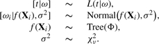where Tree(•) encompasses all the priors and distributional assumptions detailed in the above paragraph.

2.2 Ensemble-based Weibull regression

The Weibull model is parametric and used extensively to describe lifetimes, and can be reparameterized as both a CPH and an AFT model (Klein and Moeschberger, 1997). The Weibull distribution is indexed by a shape parameter τ and scale parameter ψ_i, and models the probability of survival at time t_i for patient i as

Reparametrizing the scale parameters as ω_i=log(ψ_i), the Weibull likelihood can be written as

and the survival function as S(t_i|τ, ω_i)=exp(−exp(ω_i)t_i^τ). Letting Δ=∑δ_i represent the number of censored observations, the joint likelihood function for the parameter τ and the vector of parameters ω=(ω₁,…, ω_n) becomes

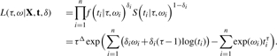As in the previous section, we model the covariate effects using a latent variable formulation, as ω_i~Normal(f(X_i), σ²), and use BART to model f. We complete our hierarchical model by assigning a conjugate gamma prior on τ as Gamma(τ_o, k_o), with fixed but vague hyperparameters. Thus, our ensemble-based Weibull regression model can be concisely written (following the above notations) as,

2.3 Ensemble-based accelerated failure time model

The AFT model is a parametric survival model that assumes that the individual survival time t_i depends on the multiplicative effect of an unknown function of covariates f(X_i) over a baseline survival time α. The AFT model (on log scale) can be written as,

where f captures the covariate effects affecting the (log) survival time directly.

We assume that the random errors, ϵ's, are normally distributed; however, we can easily adopt other distributions such as an extreme value or t distribution (Klein and Moeschberger, 1997). Note that under an extreme value distribution, the AFT model is equivalent to the Weibull model described previously.

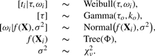
As before, let ω be a latent variable such that ω_i=f(X_i)+ϵ_i, where the ϵ_i's are i.i.d Normal(0, σ²). The AFT model can then be expressed using the data augmentation approach of Tanner and Wong (1987) to impute the censored values as,

where α is assigned a conjugate normal prior distribution as Normal(α_o, α_c), where α_o and α_c are fixed hyperparameters.

Thus, our ensemble-based AFT model can be succinctly written as

2.4 Model fitting via MCMC

We use MCMC (Gilks et al., 1996) algorithms to generate samples from the posterior distributions. The full conditionals for all three models, CPH, Weibull and AFT, as well as some examples of MCMC chains and computation times can be accessed via the Supplementary Materials. In addition, the algorithm for the proposed models is made available in R language at http://works.bepress.com/veera/1/. The specific drawing scheme for the CPH model uses a Gibbs sampler to estimate the set of parameters (ω, Φ, σ²). Gibbs sampling iterates k=1,…, K times through the following steps:

1. update Φ using the Bayesian backfitting MCMC algorithm described in CGM;

2. update σ²|Φ using a Gibbs sampler;

3. update [ω_i|Φ, σ²], where i=1,…, n, using for each ω_i a Metropolis–Hastings procedure with a proposal density q(ω_i, ω_i^*) that generates moves from the current state ω_i to a new state ω_i^*. The probability of accepting the change is given by

   

The posterior distributions of the Weibull model parameters (ω, Φ, τ, σ²) are obtained in a similar manner:

1. update Φ using the Bayesian backfitting MCMC algorithm described in CGM;

2. update σ²|Φ using a Gibbs sampler;

3. update [ω_i|Φ, τ, σ²] componentwise, where i=1,…, n, using for each ω_i a similar Metropolis–Hastings procedure with the probability of accepting the change given by

   
4. update [τ|ω, Φ, σ²] using the Metropolis–Hastings procedure with the acceptance probability given by

   

The drawing scheme for the AFT model parameters ω, α, σ² follows five steps:

1. update Φ using the Bayesian backfitting MCMC algorithm described in CGM;

2. update σ²|Φ using a Gibbs sampler;

3. obtain [α|Φ, σ², t];

4. update ω_i if δ_i=1;

5. sample from a Normal(α+ω_i, σ²) truncated at t_i if δ_i=0.

2.5 FDR-based variable selection for Ensemble-based models

One of the key goals of gene expression data analysis is selection of important predictive genes. As stated previously, BART offers a model-free mechanism for variable/gene selection. Once we apply the MCMC methods described in Section 2.4, we are left with posterior samples of the model parameters that we can use to perform Bayesian inference. The MCMC samples explore the distribution of possible tree configurations suggested by the data, with each configuration leading to a different sets of genes. Some gene configurations that are strongly supported by the data may appear in most of the MCMC samples, while others with less evidence may appear less often. There are different ways to summarize this information in the samples. One could choose the most likely (posterior mode) configuration and conduct conditional inference on this particular gene set. The benefit of this approach would be the yielding of a single set of defined genes, but the drawback is that the most likely configuration might still only appear in a very small proportion of MCMC samples. Alternatively, one could use all of the MCMC samples and, using Bayesian model averaging, mix the inference over the various configurations visited by the sampler. This approach better accounts for the uncertainty in the data, leads to estimators with the smallest prediction error and should lead to better predictive performance. We will use this Bayesian model averaging approach.

Suppose from our MCMC, we have K posterior samples of the corresponding parameter set. Let p_j denote the posterior probability of the inclusion of the j-th gene, represented by γ_j, in the model with j=1,…, p. We approximate p_j based on the relative frequency of occurrence, ø_ik, of the i-th gene across the k MCMC samples as

where ø_ik is the indicator function I(γ_j ∈ X^(k)), and X^(k) is the set of covariates used to the build the tree model in the k-th MCMC iteration. Note that (1 − p_j) can be interpreted as Bayesian q-values, or estimates of the local false discovery rate (FDR; Newton et al. 2004; Storey 2003) as they measure the probability of a false positive if the j-th gene is called a discovery or is significant. Given a desired global FDR bound α ∈ (0, 1), we can determine a threshold ϕ_α to flag a set of genes 𝒳_ϕα={j:p_j > ϕ_α} as significant. The significance threshold ϕ_α can be determined based on classical Bayesian utility considerations, such as in Müller et al. (2004), based on the elicited relative costs of false positive and false negative errors or can be set to control the average Bayesian FDR as in Morris et al. (2008), which we follow here. For example, suppose we are interested in finding the value ϕ_α that controls the overall average FDR at some level α, meaning that we expect only 100α% of the genes to be declared as significant are in fact false positives. For all genes γ_j, j=1,…,p, we sort p_j in descending order to yield p_(j), j=1,…, p. Next, ϕ_α=p_(ξ), where ξ=max[j*:(j*)⁻¹ ∑^j*_j=1 {1 − ∑ p_(j)}≤α]. Then we can claim the set of genes 𝒳_ϕα to be significant corresponding to an expected Bayesian FDR of α.

3 PERFORMANCE ASSESSMENT

We assess the performance of our method using cross-validation, i.e. we randomly split the data into mutually exclusive training and test sets in a fixed proportion, build the predictor using the training set, and then predict survival for the test set and compare it with the observed survival. In the absence of a single standard measure of prediction performance in survival models, we use three measures that assess multiple characteristics of the goodness of fit and provide our clinical collaborators meaningful outcome interpretations: the Brier score (BS), the coefficient of determination (R²) and the concordance index (CI). Several studies have shown that that these metrics are very good descriptors of predictive performance. (Harrell, 2001; Schumacher et al., 2007; van Wieringen et al., 2009). We discuss each of these measures in detail. The BS is a specialized measure of goodness-of-fit for survival models (Graf et al., 1999) that compares the observed and estimated survival functions. The BS is given by

where is the Kaplan–Meier estimate of the survival distribution for the observations (t₁,…, t_n) and I denotes an indicator function. For the BS, we utilize the training data t and X to fit a model p(t|X), and employ it to obtain the survival distribution for a future patient with covariate X_*. The BS ranges from 0 to 1; the smaller the score, the better the fit.

The R² measure is the usual coefficient of determination of the fitted model and quantifies the proportion of variability observed in the test set that can be explained by the predictor. R² is estimated as

where L(•) denotes the log-likelihood function evaluated at a particular value. In order to obtain the R², we use the median of the posterior distribution to estimate , the vector of the latent covariate effects and then we use it as a predictor in the univariable version of the specific underlying model. For example, the vector estimated from the ensemble version of the AFT model is used as the predictor vector in a univariable AFT. R² also ranges from 0 to 1 and a predictor that explains a high proportion of variability in the survival data will have R² values close to 1.

The CI can be expressed in the form

where if or 0 if otherwise, is based on pairwise comparisons between the prognostic scores and for patients i and j, respectively, and Ω consists of all the pairs of patients {i, j}. The close the CI is to 1, the better is the fit.

3.1 Breast cancer data

We compared the performance of our method with other survival prediction methods tailored for gene expression data as recently reviewed by van Wieringen et al. (2009) and other popular survival methods. We used the breast cancer dataset of Van't Veer et al. (2002; http://www.rii.com/publications/2002/vantveer.html), which contains gene expression profiles for 295 breast cancer patients and 5057 gene expression values, along with patient survival outcomes. Around 73% of these observations are right censored. Patient age ranges from 26 to 53 years and the percentage of patients with tumor grade I is 34%, grade II is 40% and grade III is 26%. We reapplied the ‘best’ methods found by van Wieringen et al. (2009): multivariable linear CPH model (CPH), L1-penalized Cox regression (CPH-L1) of Tibshirani (1997) and the L2-penalized Cox regression (CPH-L2) of Gui and Li (2005). We replicate the same setup used by van Wieringen et al. (2009) to allow comparisons across studies, i.e. we use the multivariable linear CPH model, in which the top 10 genes were obtained using a univariable Cox regression. In addition, we ran a multivariable linear Weibull model, in which the top 10 most significant genes were obtained by univariable Weibull models. We also used a multivariable linear AFT model, in which the top 10 genes were pre-selected by using a univariable AFT analysis. We also included conditional inference tree ensemble methods as Bagging, Random Forest (Hothorn et al., 2006) and Random Survival Forests (ntree=2000; Ishwaran et al., 2008) as well as CoxBoost (Binder & Schumacher, 2009). Bagging and Random Forest models were also studied by van Wieringen et al. (2009). Similarly to van Wieringen et al. (2009), we used the top 200 most significant genes obtained by the underlying univariable model to run our ensemble versions of the accelerated failure time model (AFT-TREE), the Weibull model (WEI-TREE) and the CPH model (CPH-TREE). We used a long single chain of K=10 000 iterations for each survival model with a burn-in of the first 5000 samples. In addition, we ran several chains with different initial values and found that our results are robust to these convergence checks. We repeated the cross-validation procedure 50 times with the data randomly split into training and test sets in a 2:1 ratio and with the number of censored observations kept balanced between training and test sets. We used the training set to build the predictor and then used the test set to assess the performance of the competing methods.

Based on the BS, our proposed ensemble-based methods outperformed most of the competing methods. The median BS for the ensemble method is roughly 10% smaller than those for the CPH-L1 and CPH-L2 methods, which were reported to be the best performing methods by van Wieringen et al. (2009). The best median BS is for the AFT-TREE model (0.158), followed by WEI-TREE (0.160). The median BS for CPH-TREE (0.164) model is also small and close to the medians of CoxBoost (0.162) and Bagging (0.165) methods. In terms of R², the AFT-TREE (0.141) model seems to have performance equivalent to CoxBoost (0.145) and RSF (0.146) methods while CPH- and Weibull-TREE methods did not perform as well. For the CI, all methods seem to have equivalent performance leaded by AFT (0.603) and CoxBoost (0.600) methods. The performance of some or all proposed tree-based models (0.582–0.598) is better than the performance of RSF (0.571), CPH-L1 (0.582) and RF (0.583) (see Supplementary Material for detailed information). Based on these three evaluation measures, our proposed method improves survival prediction accuracy in some cases or is, at least, equivalent in performance to competing methods. We believe that this improvement may be attributable to added flexibility when accounting for additive and non-linear effects.

We use a Bayesian FDR cutoff of 0.1 to select significant covariates for survival prediction (explained in Section 2.5) and, as a result, we found that a total of 9 variables were significant in the CPH-TREE, 7 in the WEI-TREE and 12 in the AFT-TREE. One gene (BCL2) was simultaneously listed for the AFT-TREE and the WEI-TREE. Genes identified by the models represent promising targets for further biological investigation as, for example, BCL2 gene which is one of the strongest predictors of shorter survival among breast cancer patients and was also reported by Van't Veer et al. (2002) or STK12 gene which is located in a region frequently deleted in tumors, which contains tumor-related genes such as p53 (Tatsuka et al., 1998). More details and results are presented in the Supplementary Material.

4 APPLICATION TO BRAIN TUMOR DATA

We applied the proposed method to a dataset containing gene expression profiles of brain tumors in order to identify molecular and genetic signatures that could be of prognostic value. The dataset contains gene expression measurements and survival information for 734 patients that were obtained from nine different cancer treatment centers (Broom et al., 2010). The post-diagnosis survival time of the patients with brain tumors ranges from 1 to 698 weeks, with 15% of the observations censored. Patient age ranges from 14 to 86 years and the percentage of patients with tumor grade II is 6%, grade III is 16% and grade IV is 78%. The gene expression data were obtained using three different Affymetrix microarray chips (HT-U133A, U133A and U133Plus2) and was pre-processed using a customized CDF file (Brain Array Lab, University of Michigan, see brainarray.mbni.med.umich.edu), which combines in a single expression measure the signal intensities of probesets targeting a particular gene. A total of 11 911 genes common to these three platforms was then selected and batch normalized (JMP Genomics SAS^®) to remove batch effects.

In practice, we are often interested in clusters containing correlated genes with very similar measurements in all samples. One use of these clusters is to infer the relatedness of individual genes from their membership in a common cluster. A second use is to suggest possible functions for individual genes of interest, based on the functions of other variables in the cluster, and to suggest additional related genes that might also be of interest. A third use is to calculate a cluster metagene for each sample by averaging the individual genes in the cluster. The cluster metagenes might yield more robust measurements and tests of sample characteristics than the individual variables. Converting the individual genes into metagenes also reduces the number of variables, and makes searching high dimensional spaces for interaction effects more tractable. Since our main interest is in finding prognostic groups of correlated genes, we focus our analysis on a set of metagenes that we obtained by applying an unsupervised clustering algorithm, gene shaving (Hastie et al., 2000). Gene shaving is an established method for generating such clusters. Gene shaving identifies the largest principal component, clusters the genes highly correlated with it and shaves out the less correlated genes. After finding the largest principal component, the procedure repeats until it has obtained a maximum number of clusters chosen a priori. The metagenes are then constructed from the clusters, which are assigned according to the (signed) average gene expression of their members. Using this procedure, we found 142 metagenes for downstream analysis via our ensemble-based method. In addition to the metagenes, we added clinical covariates to the survival model that included patient age and histopathological tumor grade (coded as II, III or IV). All our inferences are based on one long run of 10 000 MCMC samples, discarding the first 5000 as burn-in.

The median BS calculated for the proposed tree-based models are similar to the median BS for other models, all of them around 0.11, which indicates a good model fit. In terms of medians of R², the tree-based method CPH-TREE (0.218) and CoxBoost (0.218) figure as the best models followed by RF (0.214) and AFT-TREE and SRF (both with median 0.212). For the CI, all methods seem to have equivalent performance leaded by AFT-TREE (0.618). In general, the performance of the proposed tree-based models (0.608–0.618) is better than the performance of other tree-based methods as SRF (0.609), RF (0.614) and Bagging (0.601) (see Supplementary Material for detailed information).

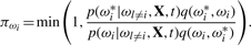
The posterior probabilities of the covariates used by our models are shown in Figure 1 along with the BFDR cut-off at α=0.1. The significant covariates for what are above this cut-off are shown in Table 1. There is a significant overlap in the metagenes and clinical covariates found by all three methods. In addition, the top five covariates mostly used by the AFT-TREE and WEI-TREE models are the same (although in different order). Tumor grade, one of the most important clinical factors for predicting survival of patients with brain tumors (The Cancer Genome Atlas Network, 2008), was confirmed in our results as one of the covariates more frequently used by all the models. Patient age, another important clinical covariate (The Cancer Genome Atlas Network, 2008), is also among the top covariates for the AFT-TREE and WEI-TREE models. In all the models, we found metagenes 52 and 99 had the highest posterior probabilities of inclusion. A search of the OMIM database (http://www.ncbi.nlm.nih.gov/omim/) revealed that these metagenes include genes known to be associated with the development and progression of tumors, including many associated with brain tissue. For example, metagene 52 includes four genes that are associated with glioma phenotypes: PHLPP, GRIPE, PIK3R1 and BAI3. PHLPP is known for its capacity to dephosphorylate Akt, triggering apoptosis and suppressing tumor growth via the p53 and RTK mitogenic pathways. PHLPP appears downregulated in several colon cancer and glioblastoma cell lines (Gao et al., 2005). Upregulation of GRIPE induces neuronal differentiation (Heng and Tan, 2002) and, therefore, prevents cells going through migration or invasion processes, resulting in good prognosis gliomas. Further, alterations of the PIK3R1 signaling pathway are present in close to 90% of glioblastomas (Cancer and Genome Atlas Network, 2008). Likewise, BAI3 is an inhibitor of angiogeneses and its downregulation is linked to an increasing of tumor vascularization, a marked characteristic of high-grade gliomas as Glioblastoma Multiforme (Shiratsuchi et al., 1997). In addition, metagene 82 includes the gene MXI1, which negatively regulates the MYC oncoprotein, an important glioblastoma tumor inductor (Albarosa et al., 1995). The downregulation of MXI1 causes the overexpression of MYC that activates cell proliferation, deactivates apoptosis (controls the death receptor Bcl-2) and triggers the mesenchymal phenotype in high-grade gliomas (Albarosa et al., 1995). In addition, metagene 70 includes the EGFR gene, which is one of the most important genes related to the development of gliomas (The Cancer Genome Atlas Network, 2008) and its upregulation triggers cell proliferation and migration processes, noticeable characteristics of poor prognosis gliomas (Wang et al., 2004).

Fig. 1.

Posterior probability of a variable appearing in the CPH-TREE (top), WEI-TREE (center) and AFT-TREE (bottom) survival ensemble methods as applied to the brain tumor data. Variables with posterior probability above the horizontal gray line are considered to be significantly used; controlled by 10% FDR. High-resolution version of this figure can be viewed in the supplementary materials.

Table 1.

Covariates significantly used in the ensemble-tree models controlling the BFDR at 10% sorted by their posterior probabilities of inclusion in the model

AFT	Weibull	CPH
metagene99a	Tumor grade	Tumor grade
Tumor grade	metagene99a	metagene52b
Patient age	metagene82b	metagene99a
metagene82b	metagene52b
metagene52b	Patient age

^aContains cancer-related genes.

^bContains glioma-related genes.

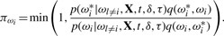
In addition to selecting relevant covariates, one of the by-products of BART are partial dependence functions (Friedman, 2001), which summarize the marginal effect of the relevant covariate s on the response. One can partition f(x) into f(x)=f(x_s, x_c) where x_s represents the predictor of interest and x_c its complement. The marginalization is obtained as where x_ic is the i-th observation of x_c in the data. The posterior distribution (post burn-in) of f(x_s) can then be used to estimate the marginal effect of s as well as its confidence intervals. Partial dependence plots are particularly useful to illustrate the marginal effect of a relevant covariate directly on survival outcome, especially in the AFT-TREE model. A plot of the partial dependence functions (Fig. 2) shows that relative upregulation of metagene 82 (variation in the x-axis) increases the survival of patients with brain tumors to roughly 170 weeks or 3.3 years (variation in the y-axis). Nomograms are another important tool fairly used by clinicians to identify the individual contributions of the covariates on patient survival. Nomograms are two-dimensional plots designed to show marginal effects of a relevant unfixed covariate while the other 1 − p non-relevant covariates remain fixed. In Figure 2, we show a nomogram of the most important variables in the AFT-TREE model. The nomogram is interpreted as follows: (i) identify the patient's age and draw a vertical line to the ‘Points’ scale at the top of the nomogram. Repeat this process for the remaining variables; (ii) sum the points for each individual variable and locate the sum on the ‘Total Points’ scale at the bottom of the nomogram. The width of a variable scale represents how much it affects the overall survival time; (iii) to calculate the survival time in weeks, draw a vertical line from the ‘Total Points’ spot on the linear predictor scale.

Fig. 2.

Marginal effects of significant covariates. Left panel: partial dependence function plots for metagene 82 with y-axis in weeks. Right panel: nomogram of the most important variables in the AFT-TREE model. High-resolution version of this figure can be viewed in the supplementary materials.

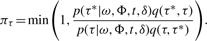
To evaluate the predictive accuracy of our methods, we used the same setup designed for the breast cancer data, i.e. we performed a cross-validation procedure with the data randomly split 50 times into training and test sets at a 2:1 ratio. First, we built the predictor using the training set. Then, we assessed and compared the performance of different methods using evaluation measures calculated for the test set. To evaluate the predictive ability of the proposed models, we conducted a time-dependent area under the curve (AUC) analysis (Fig. 3) that compares the prognostic capacity of the survival models across different binary splits of the survival response. The clinical literature reports frequent use of the time-dependent AUC analysis (Cerhan et al., 2007) to help physicians better categorize patients in terms of survival classes. In our study, the proposed ensemble methods performed better than the competing methods and demonstrated higher sensitivity.

Fig. 3.

Time-dependent AUC analysis. The plots compare the performance of the proposed tree-ensemble methods with their multivariable linear versions, as applied to the brain tumor data. Dots represent the medians across splits of training/test sets; lines depict the interquartile limits. Left plot: CPH (dashed lines) and CPH-TREE (solid lines); center plot: Weibull (dashed) and WEI-TREE (solid); right plot: AFT (dashed) and AFT-TREE (solid). High-resolution version of this figure can be viewed in the supplementary materials.

In conclusion, our results show that the clinical covariates and the expression values of few (meta)genes impact the overall survival of patients with brain tumors. We believe that these genes might be worthy of further scientific investigation, especially as potential therapeutic targets.

5 DISCUSSION

We propose Bayesian ensemble methods for survival prediction for high-throughput data such as gene expression data. Using a powerful predictive tool, BART, we model the covariate effects via a latent variable scheme, that not only allows stochastic deviations from the parameteric model but also greatly reduces the computational complexity. We chose BART because it has the flexibility to accommodate a high number of covariates and their interactions. In addition, our primary reason of working under a Bayesian paradigm is that the uncertainty in estimation is propagated at each stage of the hierarchy, thus the credible intervals on all our model parameters are in some sense exact by conditioning on all sources of variation. Thus, using the selected gene expression profile one can estimate the median survival time and credibility intervals for a given patient using the posterior distributions of the process parameters obtained with the AFT-TREE model or, alternatively, survival curves along with confidence bounds for the population using the WEI-TREE and CPH-TREE methods. Although our method is based on the BART formulation, our framework can be extended to allow for the use of any other ensemble method.

Our primary motivation of using gene sets for the brain tumor dataset was that we were more interested in groups of common genes that predict survival rather than individual genes. These genesets can be derived in various ways either using prior pathway knowledge [e.g. gene ontololgy (GO) or Kyoto Encyclopedia of Genes and Genomes (KEGG) databases] or using data-driven methods for finding clusters of correlated genes with very similar measurements in all samples, such as gene shaving. Although our methods can accommodate both scenarios, we choose the latter since it allows to infer the relatedness of individual genes from their membership in a common cluster as well as to suggest possible functions for individual genes of interest, based on the functions of other variables in the cluster, and to suggest additional related genes that might also be of interest.

The screening ability of the BART identifies important predictors across trees and training test splits of data, which allowed the model to reveal the impact of many important genes and clinical covariates on the survival of cancer patients. The application of our method to two different datasets showed that the prediction accuracy of our model outperforms that of many available models. In addition, the variable selection procedure, partial dependence functions and nomogram techniques imbue the final model with a high level of interpretability. We have a highly efficient R package available at http://works.bepress.com/veera/1/. A limitation of our proposed method is the lack of interpretability as compared to simpler regression models which is, at least, counterbalanced by gains in prediction accuracy and the ability to incorporate complex interaction effects among the covariates.

We note that the number of regression trees M set for the tree-ensemble methods dictates how often a covariate will be selected to be part of the model. Chipman et al. (2010) showed that setting a relatively small number of trees benefits the variable selection procedure since variables compete with each other to improve fit and therefore, relevant predictors should appear more frequently in the tree model. Because we were interested in exploring the BART variable selection feature, we set the number of trees M=40, which also reduces computation time without losing predictive performance. A more detailed study of the adequate number of trees can be found in the Supplementary Material.

Although motivated by a gene expression dataset, our methodology can be applied to other genomic data as well such as array-based comparative genomic hybridization and SNP data. This is so, since we do not assume any structure on the covariate space—via a ensemble formulation that accommodates complex combination of continuous and categorical predictors. We leave this task for future consideration.

REFERENCES

- Albarosa R, et al. Redefinition of the coding sequence of the MXI1 gene and identification of a polymorphic repeat in the 3-prime non-coding region that allows the detection of loss of heterozygosity of chromosome 10q25 in glioblastomas. Hum. Genet. 1995;95:709–711. doi: 10.1007/BF00209493. [DOI] [PubMed] [Google Scholar]
- Berchuck A, et al. Patterns of gene expression that characterize long-term survival in advanced stage serous ovarian cancers. Clin. Cancer Res. 2005;11:3686–3696. doi: 10.1158/1078-0432.CCR-04-2398. [DOI] [PubMed] [Google Scholar]
- Binder H, Schumacher M. Incorporating pathway information into boosting estimation of high-dimensional risk prediction models. BMC Bioinformatics. 2009;10:18. doi: 10.1186/1471-2105-10-18. [DOI] [PMC free article] [PubMed] [Google Scholar]
- Breiman L. Bagging predictors. Mach. Learn. 1996;24:123–140. [Google Scholar]
- Breiman L. Random forests. Mach. Learn. 2001;45:5–32. [Google Scholar]
- Broom BM, et al. Bagged gene shaving for the robust clustering of high-throughput data. Int. J. Bioinformatics Res. Appl. 2010;6:326–343. doi: 10.1504/IJBRA.2010.035997. [DOI] [PMC free article] [PubMed] [Google Scholar]
- The Cancer Genome Atlas Research Network. Comprehensive genomic characterization defines human glioblastoma genes and core pathways. Nature. 2008;455:1061–1068. doi: 10.1038/nature07385. [DOI] [PMC free article] [PubMed] [Google Scholar]
- Cerhan JR, et al. Prognostic significance of host immune gene polymorphisms in follicular lymphoma survival. Blood. 2007;109:5439–5446. doi: 10.1182/blood-2006-11-058040. [DOI] [PMC free article] [PubMed] [Google Scholar]
- Chipman HA, et al. Bayesian CART model search (with discussion) J. Am. Stat. Assoc. 1998;93:935–960. [Google Scholar]
- Chipman HA, et al. BART: Bayesian Additive Regression Trees. Ann. Appl. Stat. 2010;4:266–298. [Google Scholar]
- Clarke J, West M. Bayesian Weibull tree models for survival analysis of clinico-genomic data. Stat. Methodol. 2008;5:238–262. doi: 10.1016/j.stamet.2007.09.003. [DOI] [PMC free article] [PubMed] [Google Scholar]
- Cox D. Regression models and life tables. J. R. Stat. Soc. B. 1972;34:187–220. [Google Scholar]
- Datta S, et al. Predicting patient survival from microarray data by accelerated failure time modeling using partial least squares and LASSO. Biometrics. 2007;63:259–271. doi: 10.1111/j.1541-0420.2006.00660.x. [DOI] [PubMed] [Google Scholar]
- Denison D, et al. A Bayesian CART algorithm. Biometrika. 1998;85:363–377. [Google Scholar]
- D'haeseleer P. How does gene expression clustering work? Nat. Biotechnol. 2005;23:1499–1501. doi: 10.1038/nbt1205-1499. [DOI] [PubMed] [Google Scholar]
- Friedman JH. Greedy function approximation: a gradient boosting machine. Ann. Stat. 2001;29:1189–1232. [Google Scholar]
- Gao T, et al. PHLPP: a phosphatase that directly dephosphorylates Akt, promotes apoptosis, and suppresses tumor growth. Mol. Cell. 2005;18:13–24. doi: 10.1016/j.molcel.2005.03.008. [DOI] [PubMed] [Google Scholar]
- Gilks WR, et al. Markov Chain Monte Carlo in Practice: Interdisciplinary Statistics. New York: Chapman & Hall; 1996. [Google Scholar]
- Graf E, et al. Assessment and comparison of prognostic classification schemes for survival data. Stat. Med. 1999;18:2529–2545. doi: 10.1002/(sici)1097-0258(19990915/30)18:17/18<2529::aid-sim274>3.0.co;2-5. [DOI] [PubMed] [Google Scholar]
- Gui J, Li H. Penalized Cox regression analysis in the high-dimensional and low-sample size settings, with applications to microarray gene expression data. Bioinformatics. 2005;21:3001–3008. doi: 10.1093/bioinformatics/bti422. [DOI] [PubMed] [Google Scholar]
- Harrell FE. Regression modeling strategies, with applications to linear models, survival analysis and logistic regression. New York: Springer; 2001. 2001. [Google Scholar]
- Hastie T, et al. ‘Gene shaving’ as a method for identifying distinct sets of genes with similar expression patterns. Genome Biol. 2000;1 doi: 10.1186/gb-2000-1-2-research0003. RESEARCH0003. [DOI] [PMC free article] [PubMed] [Google Scholar]
- Heng JI, Tan S-S. Cloning and characterization of GRIPE, a novel interacting partner of the transcription factor E12 in developing mouse forebrain. J. Biol. Chem. 2002;277:43152–43159. doi: 10.1074/jbc.M204858200. [DOI] [PubMed] [Google Scholar]
- Hothorn T, et al. Bagging survival trees. Stat. Med. 2004;23:77–91. doi: 10.1002/sim.1593. [DOI] [PubMed] [Google Scholar]
- Hothorn T, et al. Survival ensembles. Biostatistics. 2006;7:355–373. doi: 10.1093/biostatistics/kxj011. [DOI] [PubMed] [Google Scholar]
- Ibrahim JG, et al. Bayesian Survival Analysis. New York: Springer; 2001. [Google Scholar]
- Ishwaran H, et al. Relative risk forests for exercise heart rate recovery as a predictor of mortality. J. Am. Stat. Assoc. 2004;99:591–600. [Google Scholar]
- Ishwaran H, et al. Random survival forests. Ann. Appl. Stat. 2008;2:841–860. [Google Scholar]
- Kalbfleisch JD. Non-parametric Bayesian analysis of survival time data. J. R. Stat. Soc. B. 1978;40:214–221. [Google Scholar]
- Klein JP, Moeschberger ML. Survival Analysis - Techniques for Censored and Truncated Data. New York: Springer; 1997. [Google Scholar]
- Lee KE, Mallick BK. Bayesian methods for variable selection in survival models with application to DNA microarray data. Sankhya. 2004;66:756–778. [Google Scholar]
- Lee JW, et al. An extensive comparison of recent classification tools applied to microarray data. Comput. Stat. Data Anal. 2005;48:869–885. [Google Scholar]
- Li H, Gui J. Partial Cox regression analysis for high-dimensional microarray gene expression data. Bioinformatics. 2004;20:i208–i215. doi: 10.1093/bioinformatics/bth900. [DOI] [PubMed] [Google Scholar]
- Morris JS, et al. Bayesian analysis of mass spectrometry data using wavelet-based functional mixed models. Biometrics. 2008;64:479–489. doi: 10.1111/j.1541-0420.2007.00895.x. [DOI] [PMC free article] [PubMed] [Google Scholar]
- Müeller P, Parmigiani G, Robert C, Rousseau J. Optimal sample size for multiple testing: the case of gene expression microarrays. J. Am. Stat. Assoc. 2004;99:990–1001. [Google Scholar]
- Newton MA, et al. Detecting differential gene expression with a semiparametric hierarchical mixture method. Biostatistics. 2004;5:155–176. doi: 10.1093/biostatistics/5.2.155. [DOI] [PubMed] [Google Scholar]
- Nguyen DV, Rocke DM. Partial least squares proportional hazard regression for application to DNA microarray survival data. Bioinformatics. 2002;18:1625–1632. doi: 10.1093/bioinformatics/18.12.1625. [DOI] [PubMed] [Google Scholar]
- Park PJ, et al. Linking gene expression data with patient survival times using partial least squares. Bioinformatics. 2002;18:S120–S127. doi: 10.1093/bioinformatics/18.suppl_1.s120. [DOI] [PubMed] [Google Scholar]
- Pittman J, et al. Bayesian analysis of binary prediction tree models for retrospectively sampled outcomes. Biostatistics. 2004;5:587–601. doi: 10.1093/biostatistics/kxh011. [DOI] [PubMed] [Google Scholar]
- Ross JS. Multigene classifiers, prognostic factors, and predictors of breast cancer clinical outcome. Adv. Anat. Pathol. 2009;16:204–215. doi: 10.1097/PAP.0b013e3181a9d4bf. [DOI] [PubMed] [Google Scholar]
- Schmid M, Hothorn T. Flexible boosting of accelerated failure time models. BMC Bioinformatics. 2008;9:269. doi: 10.1186/1471-2105-9-269. [DOI] [PMC free article] [PubMed] [Google Scholar]
- Schumacher M, et al. Assessment of survival prediction models based on microarray data. Bioinformatics. 2007;23:1768–1774. doi: 10.1093/bioinformatics/btm232. [DOI] [PubMed] [Google Scholar]
- Sha N, et al. Bayesian variable selection for the analysis of microarray data with censored outcomes. Bioinformatics. 2006;22:2262–2268. doi: 10.1093/bioinformatics/btl362. [DOI] [PubMed] [Google Scholar]
- Shiratsuchi T, et al. Cloning and characterization of BAI2 and BAI3, novel genes homologous to brain-specific angiogenesis inhibitor 1 (BAI1) Cytogenet. Cell Genet. 1997;79:103–108. doi: 10.1159/000134693. [DOI] [PubMed] [Google Scholar]
- Storey JD. The positive false discovery rate: a Bayesian interpretation and the q-value. Ann. Stat. 2003;31:2013–2035. [Google Scholar]
- Tanner T, Wong W. The calculation of posterior distributions by data augmentation. J. Am. Stat. Assoc. 1987;82:528–549. [Google Scholar]
- Tatsuka M, et al. Multinuclearity and increased ploidy caused by overexpression of the aurora- and Ipl1-like midbody-associated protein mitotic kinase in human cancer cells. Cancer Res. 1998;58:4811–4816. [PubMed] [Google Scholar]
- Tibshirani R. The Lasso method for variable selection in the Cox model. Stat. Med. 1997;16:385–395. doi: 10.1002/(sici)1097-0258(19970228)16:4<385::aid-sim380>3.0.co;2-3. [DOI] [PubMed] [Google Scholar]
- Van't Veer LJ, et al. Gene expression profiling predicts clinical outcome of breast cancer. Nature. 2002;415:530–536. doi: 10.1038/415530a. [DOI] [PubMed] [Google Scholar]
- van Wieringen WN, et al. Survival prediction using gene expression data: a review and comparison. Comput. Stat. Data Anal. 2009;53:1590–1603. [Google Scholar]
- Wang K, et al. Epidermal growth factor receptor-deficient mice have delayed primary endochondral ossification because of defective osteoclast recruitment. J. Biol. Chem. 2004;279:53848–53856. doi: 10.1074/jbc.M403114200. [DOI] [PMC free article] [PubMed] [Google Scholar]
- West M. Bayesian factor regression models in the “large p, small n” paradigm. In: Bernardo JM, et al., editors. Bayesian Statistics 7. New York: Oxford University Press; 2003. pp. 733–742. [Google Scholar]
Associated Data
This section collects any data citations, data availability statements, or supplementary materials included in this article.