

Abstract
Recently-proposed dynamic magnetic resonance (MR) inverse imaging (InI) is a novel parallel imaging reconstruction technique capable of improving the temporal resolution of blood-oxygen-level-dependent (BOLD) contrast functional MRI (fMRI) to the order of milliseconds at the cost of moderate spatial resolution. Volumetric InI reconstructs spatial information from projection data by solving ill-posed inverse problems using simultaneous acquisitions from a RF coil array. Previously a spatial filtering technique based on linearly constrained minimum variance (LCMV) beamformer was suggested to localize the hemodynamic changes of dynamic InI data with improved spatial resolution and sensitivity. Here we report an advancement of the spatial filtering method, which combines the eigenspace projection of the measured data and the ℓ1-norm minimization of the spatial filters’ output noise amplitude, to further improve the detection power of BOLD-contrast fMRI data. Using numerical simulation and in vivo data, we demonstrate that this eigen-space linearly constrained minimum amplitude (eLCMA) beamformer can reconstruct spatiotemporal hemodynamic signals with high statistical significance values and high spatial resolution in event-related two-choice reaction time visuomotor experiments.
Keywords: event-related, fMRI, InI, visual, motor, MRI, neuroimaging, L1 norm minimization, L2 norm minimization, eigenspace projection, beamformer, spatial filter, LCMV, Maximized SNR, dSPM, inverse solution, MEG, rapid imaging
INTRODUCTION
Functional Magnetic Resonance Imaging (fMRI) has been widely adopted for noninvasive human hemodynamic brain imaging in recent years (Belliveau, Kennedy et al. 1991; Kwong, Belliveau et al. 1992). Conventional fMRI time series are measured by echo-planar imaging (EPI) (Mansfield 1977), which encodes the spatial information by fast switching of gradients leading to spatial modulation of spin precession frequencies. Subsequently, Fourier analysis of the EPI signals maps the weights of spectral components onto spatial locations to accomplish the image reconstruction. The total scan time per image is thus closely related to the time needed to complete the traversal of the k-space. Most fMRI studies use single-shot echo-planar imaging (EPI) to achieve a temporal resolution of approximately one to three seconds with the whole brain coverage, suitable for estimating hemodynamic response in the human brain. The temporal resolution for the single-shot EPI can be moderately improved by exploiting the symmetry in k-space (Noll, Nishimura et al. 1991) and the redundancy in the repetitive measurements to further accelerate the data acquisition (Jones, Haraldseth et al. 1993; van Vaals, Brummer et al. 1993; Madore, Glover et al. 1999). Alternatively, incorporating echo shifting pulse sequences with multislice EPI can also shorten the TR to 27 ms and improve fMRI temporal resolution to 250 ms for the whole head coverage (Gibson, Peters et al. 2006). Independently, parallel imaging techniques, such as image space sensitivity encoding (SENSE) (Pruessmann, Weiger et al. 1999), k-space simultaneous acquisition of spatial harmonics (SMASH) (Sodickson and Manning 1997), and generalized autocalibrating partially parallel acquisitions (GRAPPA) (Griswold, Jakob et al. 2002), have been introduced to achieve another two- to three-fold temporal acceleration based on the spatial information among channels of an RF coil array at the cost of SNR reduction. At fixed field strength, the temporal acceleration capability of parallel MRI is closely related to the number of receiving coils in an array. Without reaching the theoretical bound (Ohliger, Grant et al. 2003; Wiesinger, Boesiger et al. 2004), the number of RF coils in head coil arrays has increased from 8 to 32 and then 96 channels (de Zwart, Ledden et al. 2002; de Zwart, Ledden et al. 2004; Wiggins GC 2005a; Wiggins GC 2005b; Wiggins, Triantafyllou et al. 2006). Inspired by the similar geometric arrangement of coils in magnetoencephalography (MEG) (Hamalainen, Hari et al. 1993) and a highly parallel MR signal detection array, single-shot volumetric MR inverse imaging (InI), which was also known as MR-encephalography (MREG) (Hennig, Zhong et al. 2007), was proposed to achieve a time resolution of 100 ms and a spatial resolution of 5 – 10 mm with whole head coverage (Lin, Wald et al. 2006; Lin, Witzel et al. 2008a). Rather than employing the standard gradient switching to explicitly encode spatial information, InI uses the spatial information among channels of an RF coil array to solve a set of ill-posed inverse problems in order to achieve high temporal acceleration with sufficient signal localization.
In InI, the inverse problems are mostly ill-posed due to the limited spatial information offered by the minimally gradient-encoded acquisitions, the number of channels in an RF coil array, and the maximal spatial frequencies that can be reconstructed from the B1 profiles of different channels in a coil array at a given field strength. Previously, we have presented methods of InI reconstruction with a constraint of minimizing the power of the reconstructed image (Lin, Wald et al. 2006; Lin, Witzel et al. 2008a) and k-space data (Lin, Witzel et al. 2010). Instead of directly solving a reconstructed image, it is possible to design individual spatial filters to project data from multiple RF coil channels onto individual volumetric image voxel in order to localize the dynamic MRI signal (Lin, Witzel et al. 2008b). Historically, a spatial filter technique also known as beamforming was first developed in applications of wireless communications systems. The goal of using a beamformer is to localize measurements from an array by designing a high spatial resolution filter such that it generates a sharp pencil-like energy beam at the antenna front end pointing to the source or the destination of interest (Van Veen and Buckley 1988). Many different spatial filtering techniques have been developed for long distance wireless communications (Liberti and Rappaport 1999; Van Trees 2002; Sarkar 2003; Allen and Ghavami 2005). Linearly constrained minimum variance (LCMV) beamformer (Frost 1972) is one of the most popular spatial filtering algorithms applied to the receiver side to minimize the antenna array’s output variance with linear constraints. In addition to fMRI reconstruction (Lin, Witzel et al. 2008b), LCMV also has been extensively applied to EEG and MEG signal localization (Van Veen, Van Drongelen et al. 1997; Ishii, Shinosaki et al. 1999; Sekihara, Nagarajan et al. 2001; Sekihara, Nagarajan et al. 2002).
The LCMV spatial filter design uses the data covariance matrix estimated from the measurements of all channels. Considering the measurements include the deterministic signal part and the stochastic noise part, the variance, and thus the performance, of the spatial filter’s output is closely related to the measurement noise. If it is possible to separate “signal” and “noise” components from the measurements, it might be beneficial to design a spatial filter to localize the source with higher SNR at the output of the spatial filter. Eigenspace projection is one such method separating measurements into signal and noise components by projecting the data on to empirically estimated signal and noise eigenspaces, respectively (Van Trees 2002). The projection eigenvectors are derived from the eigenvalue decomposition of the data correlation matrix. Two orthogonal subspaces corresponding to signal and noise can then be constructed. Specifically, eigenvectors with magnitude-sorted eigenvalues higher than a pre-defined threshold constitute the signal subspace and the rest of eigenvectors span the noise subspace. The eigenspace beamformer can then be designed based on the covariance matrix of measurements projected on either signal or noise subspace. Various eigenspace beamformers have been applied to functional brain imaging over the last twenty years. Multiple Signal Classification (MUSIC) algorithm has been introduced (Schmidt 1986) and used in MEG source localization (Mosher, Lewis et al. 1992; Sekihara, Poeppel et al. 1997; Sekihara, Nagarajan et al. 1999) as well as fMRI time-course signal analysis (Sekihara and Koizumi 1996). Alternatively, it is possible to design eigenspace spatial filters to specifically minimize the output variance of the projected measurements onto the signal subspace (Sekihara 2008). It has been shown that both types of beamformers can improve SNR significantly at the receiver side with low computational cost (Van Trees 2002).
Aforementioned LCMV and eigenspace beamformers are mathematically based on minimizing the output variance of the spatial filters. This is equivalent to minimizing the ℓ2-norm least square error between the estimated and true source signals (Sekihara 2008). While source localization methods based on the constraint of minimizing the ℓ1-norm of the sources have been explored in both wireless communications (Barroso and Moura 1989; Barroso and Moura 1994) and MEG source analysis (Barroso and Moura 1989; Barroso and Moura 1994; Uutela, Hamalainen et al. 1999; Huang, Dale et al. 2006), designing a spatial filter for minimal output disturbance quantified by the ℓ1-norm, to our best knowledge, has not been discussed yet in neuroimaging analysis.
This study focuses on the development of spatial filtering of InI data using the eigenspace projection and the ℓ1-norm minimization constraint. In the following, we first review the principle of LCMV and the eigenspace LCMV (eLCMV) spatial filtering techniques (Van Veen and Buckley 1988) to reconstruct dynamic InI data for fMRI studies. Subsequently, we introduce linearly constrained minimum amplitude (LCMA) and eigenspace linearly constrained minimum amplitude (eLCMA) beamformers by replacing the minimum ℓ2-norm constraint with the ℓ1-norm constraint. We used numerical simulations to quantify the performance of the four spatial filters: LCMV, eLCMV, LCMA, and eLCMA beamformers. We also used all four spatial filters to reconstruct in vivo dynamic BOLD contrast InI during a visuomotor task. Our results demonstrate the feasibility of applying the eLCMA beamformer to localize task-related active brain areas with the advantage of high statistical t-values and less source spread.
MATERIALS AND METHODS
The data used in this study have been reported in our previous paper (Lin, Witzel et al. 2010). For the completeness of the readership, we briefly describe the experimental information here again.
Subjects
Nine (n = 9) healthy subjects, with either normal or corrected normal vision, participated in the in vivo experiment. Experiments for all subjects were under the approved condition by the Institutional Review Board of our institutes. Written consent forms were also obtained from each subject before the experiment.
Task
Our visuomotor task required the subjects to flex right hand fingers upon perceiving a high-contrast hemi field (right field) visual checkerboard reversing at 8 Hz. The motor task was sequential finger flexion between D1-D3, D1-D5, D1-D2, and D1-D4 (D1: thumb, D2: index finger, D3: middle finger, D4: ring finger, D5: little finger). The purpose of this rather complicated motor task is to elicit a stronger hemodynamic response. The checkerboard subtended 8° of visual angle and was generated from 24 evenly distributed radial wedges (15° each) and eight concentric rings of equal width. The stimuli were generated using the Psychtoolbox (Brainard 1997; Dale 1999a). The reversing checkerboard stimuli were presented in 500 ms epochs and the onset of each presentation epoch was randomized with a uniform distribution of inter-stimulus intervals varying between 3 and 16 s (average inter-stimulus-interval: 10 seconds). Twenty-four stimulation epochs were presented during four 240 s runs, resulting in a total of 96 stimulation epochs per participant. The choice for the inter-stimulus intervals varying between 3 and 16 s was made by the consideration of the duration of the HRF and practical concerns on accommodating 24 stimulus events within a 240 s run.
Image data acquisition
MRI data were collected with a 3T MRI scanner with a 32-channel coil array (Tim Trio, Siemens Medical Solutions, Erlangen, Germany). The InI reference scan was collected using a single-slice echo-planar imaging (EPI) readout, exciting one thick coronal slab covering the entire brain (FOV 256 mm × 256 mm × 256 mm; 64 × 64 × 64 image matrix) with the flip angle set to the Ernst angle of 30° for the gray matter (considering the T1 of the gray matter is 1 second at 3T). 3D phase encoded EPI acquisition was used to obtain the spatial information along the anterior-posterior axis. The EPI readout had frequency and phase encoding along the superior-inferior and left-right axes respectively. We used TR=100 ms, TE=30 ms, bandwidth=2604 Hz and a 12.8 s total acquisition time for the reference scan, consisting of 64 TRs and two repetitions allowing the coverage of a volume comprising 64 partitions. For the InI functional scans, we used the same volume prescription, TR, TE, flip angle, and bandwidth as for the InI reference scan. The principal difference was that the 3D phase encoded EPI acquisition was removed so that the full volume was excited, and the spins were spatially encoded by a single-slice EPI trajectory, resulting in a coronal X/Z projection image with spatially collapsed projection along the anterior-posterior direction. The InI reconstruction algorithm was then used to estimate the spatial information along the anterior-posterior axis. In each run, we collected 2,400 measurements after collecting 32 measurements in order to reach the longitudinal magnetization steady state. A total of 4 runs of data were acquired from each participant. In addition to the InI reference and functional scans, structural MRI data for each participant were obtained in the same session using a high-resolution T1-weighted 3D sequence (MPRAGE, TR/TE/flip = 2530 ms/3.49 ms/7°, partition thickness = 1.33 mm, matrix = 256 × 256, 128 partitions, FOV = 21 cm × 21 cm). Using these data, the location of the gray-white matter boundary for each participant was estimated with an automatic segmentation algorithm to yield a triangulated mesh model with approximately 340,000 vertices (Fischl, Sereno et al. 1999; Dale, Fischl et al. 1999b; Fischl, Liu et al. 2001). This mesh model was then used to facilitate mapping of the structural image from native anatomical space to a standard cortical surface space (Fischl, Sereno et al. 1999; Dale, Fischl et al. 1999b). To transform the functional results into this cortical surface space, the spatial registration between the InI reference and the native space anatomical data was calculated by FSL (http://www.fmrib.ox.ac.uk/fsl), estimating a 12-parameter affine transformation between the volumetric InI reference and the MPRAGE anatomical space. The resulting spatial transformation was subsequently applied to each time point of the reconstructed InI hemodynamic estimates to spatially transform the signal estimates to a standard cortical surface space (Fischl, Sereno et al. 1999; Dale, Fischl et al. 1999b).
fMRI Reconstruction
The fMRI analysis of the InI data set across all channels in an RF coil array and across all time points can be considered as two separate processing steps: 1) estimation of the hemodynamic responses from the projection data for each channel in the RF coil array, and 2) performing the volumetric reconstruction by solving the inverse problem based on the multi-channel hemodynamic response data. As discussed in our previous study, we first process the time-domain data by deconvolving the InI time series measurements with the design matrix to compute the coefficients of the HRF basis functions. Subsequently, the spatial inverse reconstruction of these basis function coefficients from all channels in the coil array is performed at each individual time frame. Under the assumption of linearity in the BOLD fMRI responses (Boynton, Engel et al. 1996), this strategy can greatly improve the computational efficiency since the time domain processing can reduce the size of the data by 8-30 folds (Lin, Witzel et al. 2010). Specifically, we used Finite-Impulse-Response (FIR) basis function of 30 s duration (6 second pre-stimulus interval) and General Linear Model (GLM) to allow a high degree of freedom in characterizing dynamic responses. Given TR=100 ms and the assumed 30 s as the duration for HRF, we had 300 unknown coefficients for the FIR basis functions. With the estimates of the coefficients of HRF basis on each channel of the coil array and at each time point, we then used the spatial filters introduced in the following section to estimate the HRF and the associated dynamic statistical parametric maps at each voxel in the brain.
InI RECONSTRUCTION THEORY
LCMV Beamformer
For the completeness of the presentation, here we briefly review the theory of linearly constrained minimum variance beamfomer and InI reconstruction. Considering the InI acquisition from a RF coil array with nR channels, we denote by y(tk) the InI measurement for one pixel in the projection image acquired by leaving out nS partition encoding steps in one volumetric field of view (FOV) at the kth time frame tk :
| (1) |
In the above equation y(tk) is a nR-by-1 measurement vector, x(tk) is a nS-by-1 source vector to be reconstructed, and n(tk) is the contaminating nR-by-1 noise vector, and A is an nR-by-nS forward matrix, which can be empirically measured from the InI reference scan (Lin, Wald et al. 2006; Lin, Witzel et al. 2008b). Each row of the forward matrix A represents one fully gradient encoded volumetric image measured at one channel of the RF coil array. Each column of A represents the measured MR signals from different channels of the coil array at one particular image voxel. Specifically in the context of InI reconstruction, the forward matrix A is different for each Fourier encoded location and each row of A corresponds to the “voxel” intensities along the omitted direction at a specific Fourier encoded location. The reference scan uses full partition encoding steps and measures the spatial sensitivity maps from all channels of the coil array in 3D. In summary, Aij indicates the jth voxel intensity of the reference scan at the ith receiving coil and a specified gradient encoded location.
The contaminating noise n(tk) can be spatially correlated among channels of a coil array. Before designing spatial filters, such spatial correlation can be first removed by a whitening process. The whitening matrix C-1/2 can be obtained by decomposing the noise covariance matrix C:
| (2) |
The whitened measurement yw(tk) then becomes:
| (3) |
, where yw(tk)= C-1/2 · y(tk), Aw= C-1/2 · A, and ⟨nw(tk) · nw(tk)T⟩ = C−1/2 · C · C−1/2 = InR. Here ⟨ · ⟩ represents the time ensemble average and InR is an nR-by- nR identity matrix.
The standard linearly constrained minimum variance (LCMV) spatial filter W with the size of nR-by-nS is then designed to minimize the output source variance:
| (4) |
Each row of WT was subject to the linear constraint:
| (5) |
, where and represent the ith row of WT and the ith column of AW, respectively.
An nR-by-nR data correlation matrix D can be empirically measured from a time interval [t1, tm]:
| (6) |
, where yw(tk) is the spatially whitened measurements defined in Eq. (3). The rank of the generated data correlation matrix should be sufficient to span a space of possible source signals. The temporal window for correlation matrix can be determined analytically if the bandwidth of the interested signal is known (Brookes, Vrba et al. 2008), or empirically by choosing a window three times longer than the number of sensors (Van Veen, van Drongelen et al. 1997). Since the bandwidth of our interested sources are not known prior to the experiment, we determine the size of the temporal window practically, which our previous InI LCMV paper used the range of [0s 8s] after stimulus onset (Lin, Witzel et al. 2008b). We choose the same duration in this experiment for the consistency of data analysis.
By introducing a Lagrange multiplier, the optimized spatial filter W can be derived analytically (Van Veen, Van Drongelen et al. 1997):
| (7) |
In practice, the duration of the whitened measurements yw may not be long enough, rendering the data correlation matrix D rank deficient. To remedy this problem, we proposed a regularization procedure (diagonal loading) to improve the condition of D (Lin, Witzel et al. 2008b):
| (8) |
Note that we are using the noise-whitened measurements, so, C = Ireg, where Ireg is an nR-by- nR identity matrix. The scalar ε can be specified by the measurement SNR (Lin, Belliveau et al. 2006; Lin, Wald et al. 2006):
| (9) |
The LCMV spatial filter then becomes:
| (10) |
The dynamic statistical parametric maps (dSPM) T(tk) for InI reconstruction value for each reconstructed pixel in the image at each time frame can be estimated from the noise-normalized spatial filter , which is derived from the ratio between the LCMV spatial filter in (10) and the estimated baseline noise. Since the measurements are already noise-whitened, C is now an identity matrix, i.e.:
| (11) |
, and
| (12) |
Eigenspace LCMV (eLCMV) Beamformer
The data correlation matrix after whitening (Eqs. (2) and (3)) ensures that the measurements are contaminated by a multivariate spatially white noise of zero mean and unit variance. However, the measurements can still be spatially correlated due to the signal part. Here we further assume that the noise-whitened measurements can be separated into orthogonal “signal” and “noise” components. Such separation can be practically done by projecting measurements into “signal” and “noise” subspaces, whose bases can be derived from the Singular Value Decomposition (SVD) of the symmetric data correlation matrix D:
| (13) |
| (14) |
| (15) |
, where λk denotes the kth magnitude sorted (in a descending order) singular values of D at the kth diagonal entry of Σ. Uk is the kth singular vector at the kth column of the matrix U. In this study, the singular vectors with singular value greater than 1.0 are considered to form the basis for the signal subspace, and singular vectors with singular value smaller than 1.0 are assumed to span the noise subspace. Namely, p is the largest number such that λp>1 (Sekihara 2008).
Since the goal of spatial filtering is to minimize the output variance, we specifically look for a spatial filter operating on the noise with minimal output. This rationale leads to the eLCMV spatial filter as the solution of the following optimization problem:
| (16) |
Each row of WT was subject to the linear constraint:
| (17) |
, where and represent the ith row of WT and the ith column of AW, respectively.
The regularized spatial filter can be derived in a similar fashion from Eq. (7)-(10):
| (18) |
, where
| (19) |
, and the scalar ε is defined in Eq. (9).
Accordingly, the baseline-normalized spatial filter can be calculated:
| (20) |
, and the InI data are reconstructed similar to Eq. (12).
Linearly Constrained Minimum Amplitude (LCMA) Beamformer
We propose a new beamformer based on the ℓ1-norm minimization of the amplitude of source output. The objective function below is used to derive the LCMA spatial filter WLCMA:
| (21) |
Each row of WT was subject to the linear constraint:
| (22) |
, where and represent the ith row of WT and the ith column of AW, respectively.
Here ∥ ■ ∥1 denotes the ℓ1-norm, and
| (23) |
Since the solution to the cost function in (21) does not have an analytical form, we solve WLCMA by using linear programming (LP). Accordingly, noise-normalized LCMA beamformer can be derived similar to Eq. (11):
| (24) |
Given the , we can reconstruct InI data time point by time point using this time-invariant spatial filter.
Eigenspace Linearly Constrained Minimum Amplitude (eLCMA) Beamformer
Following the rationale of eigenspace projection, we now propose the eLCMA spatial filter WeLCMA as the solution to minimize the following objective function:
| (25) |
Each row of WT was subject to the linear constraint:
| (26) |
, where and represent the ith row of WT and the ith column of AW, respectively, and
| (27) |
, where UN is the matrix consisting of noise subspace singular vectors and is a diagonal matrix whose diagonal entries are the square roots of the noise subspace singular values.
After solving WeLCMA numerically by linear programming (LP), the noise-normalized eLCMA beamformer can be derived similar to Eq. (11):
| (28) |
The reconstructed InI data for each time frame are obtained by multiplying the whitened measurements yw(tk) by .
Simulation
We used simulation to test the localization accuracy and the spatial resolution of the designed spatial filters. Specifically, we simulated two regions of interest (ROIs): one at the visual cortex around the Calcarine fissure, and the other one at the sensorimotor cortex across the central sulcus. The locations of these two ROIs were based on the realistic anatomy from high resolution MRI data. The simulated source vector x had a unit amplitude in all voxels within the ROI and zero otherwise. The noiseless measurement yorig was then computed by multiplying x by the forward solution A. To account for the spatial correlation among receiving coils, the “colored” additive noise n was then simulated from the white Gaussian noise nw multiplied by a “coloring matrix” C1/2, where C is the noise variance matrix. C1/2 = U · Σ1/2, U and Σ have been defined in equation (2). The magnitudes of the noiseless measurement yorig and the contaminating noise n received at each receiving coil need to be scaled properly to match the pre-assumed SNR in our simulation. The signal power at each coil was calculated by the diagonal entries in the correlation matrix , while the power of noise at each coil was calculated by the diagonal entries in the noise covariance matrix C. The estimated SNR of each coil is then the square root of the ratio between the signal power and the noise power in each coil. The noiseless measurements yorig were scaled by the assumed SNR coil by coil, with SNR varied parametrically from 1,5,10, to 30. The scaled noiseless measurements and the noise were then added together to simulate the data y contaminated by spatially correlated noise. The source reconstruction using spatial filters with noise normalization were then implemented by the procedures and equations described in the sections above.
The reconstruction performance for LCMV, eLCMV, LCMA, and eLCMA beamformers were then analyzed and compared. We used the averaged point spread function (APSF) and the SHIFT metrics reported in our previous study (Lin, Witzel et al. 2008b) to quantify the spatial resolution and the localization accuracy of different spatial filters. Specifically,
| (29) |
where |di(ρ̄)| indicates the distance between source location i and source location ρ̄. xi represents the source vector entry in the beamformer reconstruction x̄(ρ̄) whose magnitude exceeds 0.5.
| (30) |
where W is the designed spatial filter. l is the number of voxels to be spatially resolved by the InI reconstructions. This procedure allows estimation of the full-width-half-maximum (FWHM) of the point spread function. Quantification of localization accuracy was done by calculating the shift between the center of mass of InI reconstruction and the simulated source:
| (31) |
The data processing and image reconstruction for both simulated and empirical data analysis were implemented in Matlab (Mathworks, Natick, MA), and the solution to WLCMA and WeLCMA for ℓ1-norm minimization was estimated by a software called CVX, a Matlab-based modeling toolbox for discipline convex programming. Specifically, WLCMA and WeLCMA are obtained by the interior point method implemented in the CVX program (Grant and Boyd 2009).
RESULTS
The spatial distributions of the simulated sources and the reconstructed values for different noise normalized spatial filters at different simulated SNR’s are shown in Figure 1.
Figure 1.

Spatial distribution for simulated sources and reconstructed InI for the eLCMA, LCMA, eLCMV, and LCMV beamformers for different SNR’s in the sensorimotor and visual area. The display threshold for t-value was 5 (Bonferroni corrected p < 0.01).
Figure 1 shows that the eLCMA beamformer can reconstruct most sources within the visual and sensorimotor cortex ROIs with higher statistical values than the sources reconstructed by the LCMV, eLCMV and LCMA spatial filters across different SNR’s. The ratio between the peak reconstruction statistics from spatial filters and that from the LCMV are listed in Table 1. The peak of eLCMA beamformer is about 30% higher than the peak of LCMV, while both the peaks of LCMA and the eLCMV beamfomers have approximately 10% higher than the peak of LCMV reconstructions.
Table 1.
Simulated quantitative analysis for reconstructed sources: Averaged peak signal gain ratio comparison for the eLCMA, LCMA, eLCMV, and LCMV beamformers.
| Motor area: | ||||
|---|---|---|---|---|
| Averaged Peak Signal Gain Ratio | ||||
| SNR | eLCMA | LCMA | eLCMV | LCMV |
| 1 | 1.3 | 1.1 | 1.0 | 1.0 |
| 5 | 1.2 | 1.1 | 1.1 | 1.0 |
| 10 | 1.3 | 1.1 | 1.1 | 1.0 |
| 30 | 1.2 | 1.2 | 1.2 | 1.0 |
| Average | 1.3 | 1.1 | 1.1 | 1.0 |
| Visual area: | ||||
| Averaged Peak Signal Gain Ratio | ||||
| SNR | eLCMA | LCMA | eLCMV | LCMV |
| 1 | 1.3 | 1.0 | 1.0 | 1.0 |
| 5 | 1.4 | 1.1 | 1.1 | 1.0 |
| 10 | 1.3 | 1.2 | 1.2 | 1.0 |
| 30 | 1.3 | 1.2 | 1.2 | 1.0 |
| Average | 1.3 | 1.1 | 1.1 | 1.0 |
The location accuracy of the reconstructed sources was quantified by the APSF and SHIFT metrics, which were both calculated from the linearly scaled InI reconstruction between 0 and 1. Maps of APSF and SHIFT for simulated sources at the visual and sensorimotor cortex ROIs were shown in Figure 2. Across different SNR’s in both visual and sensorimotor cortex ROIs, we found that sources reconstructed by the eLCMA and LCMA beamformers have lower APSFs which indicate less signal spread than the sources reconstructed by LCMV and the eLCMV beamfromers which are spatial filters based on the minimum ℓ2-norm cost functions. Sources estimated by the eLCMA and LCMA beamformers, however, have slightly larger shift than other two beamformers in terms of the location of the center-of-mass in ROI. Nevertheless, the combined averaged signal spreads and shifts reconstructed by our proposed eLCMA and LCMA beamformer across different SNR’s are about half of the voxel size (4 mm). This implies that the localization for the reconstructed sources using the ℓ1-norm minimization is still fairly accurate with modest localization uncertainty. The localization uncertainty for the sources reconstructed by LCMV and the eLCMV spatial filters is about one voxel. Considering those two factors jointly, it can be argued that the eLCMA and LCMA spatial filters outperform other two ℓ2-norm based beamformers in terms of the accuracy of the source localizations. The APSF and SHIFT metrics for all four spatial filters under different SNR’s were reported in Table 2. Intuitively, a smaller APSF metric is expected at a higher SNR for all spatial filters. However, considering the noise sensitivity of the L1-minimization procedure, we did not observe monotonic decrease in APSF at a higher SNR in, for example, eLCMA. Such variability was actually observed in APSF for LCMA filters at different SNRs, too. We found that as SNR varied between 1 and 30, APSF in LCMA filters can vary between 1.0 and 1.6 (Table 2). Considering such variability, it might not be straight-forward to conclude that the APSF was significantly larger at higher SNR.
Figure 2.
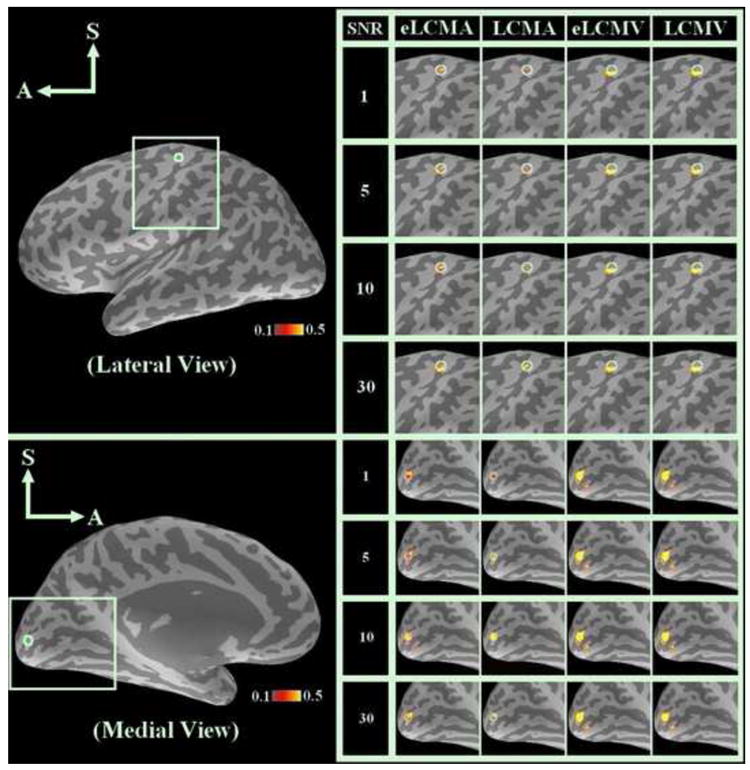
Spatial distribution for the simulated sources and scaled reconstructed InI for the eLCMA, LCMA, eLCMV, and LCMV beamformers for different SNR’s in the sensorimotor and visual cortex areas.
Table 2.
Simulated spatial distribution quantitative analysis for reconstructed sources: APSF and SHIFT for the eLCMA, LCMA, eLCMV, and LCMV beamformers.
| Motor area: | ||||||||
|---|---|---|---|---|---|---|---|---|
| APSF (mm) | SHIFT (mm) | |||||||
| SNR | eLCMA | LCMA | eLCMV | LCMV | eLCMA | LCMA | eLCMV | LCMV |
| 1 | 1.54 | 1.60 | 3.44 | 3.30 | 0.42 | 0.58 | 0.27 | 0.29 |
| 5 | 1.68 | 1.01 | 3.36 | 3.38 | 0.50 | 0.29 | 0.23 | 0.22 |
| 10 | 1.63 | 1.01 | 3.39 | 3.32 | 0.26 | 0.25 | 0.25 | 0.24 |
| 30 | 2.00 | 1.61 | 3.66 | 3.15 | 0.37 | 0.38 | 0.23 | 0.23 |
| Average | 1.71 | 1.31 | 3.47 | 3.29 | 0.39 | 0.37 | 0.25 | 0.25 |
| Visual area: | ||||||||
| APSF (mm) | SHIFT (mm) | |||||||
| SNR | eLCMA | LCMA | eLCMV | LCMV | eLCMA | LCMA | eLCMV | LCMV |
| 1 | 1.19 | 1.02 | 3.31 | 3.15 | 0.54 | 0.26 | 0.21 | 0.23 |
| 5 | 1.25 | 1.57 | 3.25 | 3.17 | 0.66 | 0.35 | 0.31 | 0.23 |
| 10 | 1.55 | 1.49 | 3.26 | 3.15 | 0.31 | 0.31 | 0.30 | 0.29 |
| 30 | 1.87 | 1.18 | 3.29 | 3.12 | 0.56 | 0.48 | 0.25 | 0.23 |
| Average | 1.46 | 1.32 | 3.28 | 3.14 | 0.52 | 0.35 | 0.27 | 0.24 |
Moreover, we found that there were “ghost” blobs at the other side of the Calcarine sulcus in Figures 1 and 2. These artifacts can be due to the rendering of volumetric reconstruction onto cortical surface. All reconstructions of four spatial filters generated such a “ghost” blob. However, Figure 1 shows results thresholded at a t statistics (t = 5) common to all reconstructions, while Figure 2 shows individually scaled reconstructions. Taken Figures 1 and 2 together, the sources reconstructed by our proposed eLCMA spatial filter, therefore, has higher statistical values and better localization accuracy than other three spatial filters explored in this study.
To examine the spatial resolution along the InI encoding axis for our proposed reconstruction methods, two temporally uncorrelated point sources with unit amplitudes around the motor area are placed along the InI encoding direction (anterior-posterior direction in this study) and separated by one, two, and three voxels, respectively. We choose SNR=5, and sources reconstructed by eLCMA, LCMA, eLCMV, and LCMV are shown in Figure 3. It can be observed in our simulation that eLCMA/LCMA can identify two separated sources as long as two point sources are located two voxels away or farther, while eLCMV/LCMV can only identify two sources when they are separated by three or more voxels. This result, therefore, shows that eLCMA and LCMA offer better spatial resolution than eLCMV/LCMV along the InI encoding direction.
Figure 3.
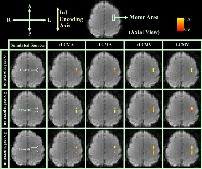
Spatial resolution simulation for two point sources with unit amplitudes (SNR=5) along InI encoding axis separated by one voxel (1st row), two voxels (2nd row), and three voxels (3rd row): (from left to right) eLCMA (1st column), LCMA (2nd column), eLCMV (3rd column), and LCMV beamformer (4th column).
Spatiotemporal localization of visuomotor hemodynamic responses
The functional areas on the cortical surface in response to the visuomotor task were examined after choosing a critical threshold for the t-statistics of 5 (Bonferroni corrected p-value < 0.01). The Bonferroni correction is a rather conservative correction for the t statistics considering the spatial smoothness of the reconstruction. Specifically, this correction was made by inflating the p values by 64, since each InI inverse problems involves 64 unknowns. The lateral view of the spatiotemporal reconstructed InI t statistic maps from the group analysis (n = 9) is shown in Figure 4. Figure 4 clearly demonstrates that the BOLD response estimated by eLCMA beamformer has a higher t statistic peak than those estimated by LCMV, eLCMV, and LCMA beamformers. Especially, reconstructed sources around the central sulcus by the eLCMA spatial filter have higher statistical values.
Figure 4.

Group analysis for InI reconstruction data around the sensorimotor area on the left hemisphere (lateral view): (from left to right) eLCMA (1st column), LCMA (2nd column), eLCMV (3rd column), and LCMV beamformer (4th column), and InI reconstruction data around the visual area on the left hemisphere (medial view): eLCMA (5th column), LCMA (6th column), eLCMV (7th column), and LCMV beamformer (8th column).
The medial view of the reconstructed spatiotemporal InI t statistic map from the group analysis (n = 9) for rendering the BOLD activity in the visual cortex is also shown in Figure 4. Similar to the results in the sensorimotor area, the source estimated by eLCMA beamformer have a higher t statistic peak than the peak t statistics estimated by the LCMA, LCMV, and eLCMV beamformers.
The group-averaged sources within the visual and sensorimotor cortex ROIs can be further compared. Sources reconstructed by four different spatial filters were linearly scaled between 0 and 1. To be consistent between simulation (Figure 2) and in vivo data analysis, we used the same threshold to render results. The spatial distributions of the scaled InI reconstructions at the time reaching maximal value are shown in Figure 5. It can be observed that sources reconstructed by the eLCMA and LCMA beamformers have less spread than the sources reconstructed by the other two beamformers. Importantly, the visual cortex activity estimated by the eLCMA and LCMA beamformers show good alignment with the Calcarine sulcus, while the reconstructions by LCMV and eLCMV beamformers report significant hemodynamic responses covering the two adjacent banks of the calcarine sulcus. Similarly, the BOLD responses at the sensorimotor area estimated by the beamformers using the ℓ1 norm minimizations are more spatially focal than those estimated by the beamformers using the ℓ2 norm minimizations. Consistent with our simulations, these results support that the eLCMA beamformer offers a higher spatial resolution.
Figure 5.

Scaled spatiotemporal reconstruction within ROI at the maximum activation time point for all spatial filters (from left to right): eLCMA (1st column), LCMA (2nd column), eLCMV (3rd column), and LCMV beamformer (4th column).
The time-courses for all four spatial filters in the sensorimotor and visual cortex areas are shown in Figure 6. In the sensorimotor and visual cortex ROIs, Figure 6a and 6b show that the peak t-value reconstructed by the eigenspace minimum ℓ1-norm beamformer are about 20-30% higher than the peak t-values reconstructed by other three beamformers. This is consistent with the simulations shown in Figure 5.
Figure 6.

A: averaged time-course result for group analysis around the sensorimotor area: eLCMA (red), LCMA (magenta), eLCMV (green), and LCMV (blue). B: averaged time-course result for group analysis around the visual area: eLCMA (red), LCMA (magenta), eLCMV (green), and LCMV (blue).
The visual and motor average response reconstructed by eLCMA beamformer can be analyzed further. The averaged hemodynamic responses of motor and visual areas were first linearly scaled between 0 and 1 and then fitted by the model proposed in (Glover 1999), respectively. The scaled and fitted BOLD time courses in both visual and sensorimotor cortex areas are shown in Figure 7. We are interested in inferring the relative timing between these two BOLD time courses and used the time reaching 0.5 (time-to-half, TTH) and the time reaching the peak (time-to-peak, TTP) as the relevant latency indices. We found the TTH is 2.0s for the visual cortex area and 2.9s for the motor cortex area, and TTPs is 3.8s and 4.7s for the visual and sensorimotor cortex areas, respectively.
Figure 7.

Normalized averaged and fitted time-course plots for both motor and visual cortex response reconstructed by eLCMA beamformer: Fitted normalized motor cortex hemodynamic response (red), and fitted normalized visual cortex hemodynamic response (blue).
To compare beamformer results with fully gradient encoded data, we report results of a separate experiment using photic stimulation with traditional multi-slice EPI and InI reconstructed by four beamformers in this revision. This data set was previously used in our InI study (Lin, Witzel et al. 2008a). The group average results (n = 6) are shown in Figure 8. Figure 8a shows the linearly scaled hemodynamic responses within the visual ROI. The normalized time course for the EPI and InI are qualitatively similar in onset, time to peak, and post-stimulus undershoot. Based on Figure 8a, Figure 8b shows the temporally averaged hemodynamic responses within [2s 8s] for EPI and InI reconstructed by different beamformers around the posterior part of the Calcarine sulcus. Quantitatively, the center of mass of LCMV, eLCMV, LCMA, and eLCMA shifted away from the center of mass of EPI results by 8.9, 8.2, 3.3, and 5.6 mm respectively. This demonstrates that the InI data reconstructed by beamformers are close to the EPI spatiotemporally.
Figure 8.

A. Normalized group averaged time course plots within ROI for EPI and InI reconstructed by four spatial filters: EPI (black), eLCMA (red), LCMA (magneta), eLCMV (green), LCMV (blue). B. Normalized spatiotemporal reconstruction for EPI and InI averaged between 2 s and 8 s for all spatial filters (from left to right): EPI (1st column), eLCMA (2nd column), LCMA (3rd column), eLCMV (4th column), and LCMV beamformer (5th column).
The selection of the threshold for separating the signal and noise subspaces has been discussed in detail previously in the context of signal processing (Van Trees 2002) and brain imaging (Sekihara 2008). As explained above, we chose this threshold to be equal to one, because the baseline “noise” has a unit power after spatial whitening. Subjectively, we considered the whitened data eigenvectors with power higher than one to be “signal”. Different eigenspace thresholds may affect the performance of the spatial filtering. Figure 9a and 9b show the average time courses of the visual and sensorimotor cortices using the eLCMA beamformer at different eigenspace thresholds. We found that the performance of the eLCMA beamformer is only marginally affected by the chosen threshold as long as the threshold is set to one or larger. To further support this observation, we plotted the descending-order eigenvalues of the data correlation matrix from the measurements for a subject in Figure 10. It can be observed from Figure 10 that eigenvalues did not change dramatically around the chosen (λ>=1) threshold. Importantly, a large proportion of eigenvalues and eigenvectors were preserved even at a high threshold, i.e. λ>=9. A higher threshold also ensures a larger rank of the noise subspace. When using a smaller threshold (for example, λ = 0.5), the rank of the noise subspace is too small to generate versatile spatial filters tailored for localizing distinct sources accurately. This is illustrated in the time course with a smaller peak t statistic using λ = 0.5 in Figure 9.
Figure 9.

A: group averaged time course plots for different thresholds (λ=0.5, 1, 4, and 9) in the motor cortex area. B: group averaged time course plots for different thresholds (λ=0.5, 1, 4, and 9) in the visual cortex area.
Figure 10.

Eigenvalue plot of the data correlation matrix for a single subject with the line indicating the threshold is set to one.
DISCUSSION
Our paper presents two features of processing the dynamic InI data using spatial filtering: eigenspace projection and the ℓ1-norm minimization. Our simulations and in vivo fMRI data analysis consistently show that the eigenspace projection can lead to higher reconstructed values statistically, while the ℓ1-norm minimization can offer better spatial resolution compared with the spatial filters using the ℓ2-norm minimization. Considering the alternatives of either minimizing the ℓ1-norm or the ℓ2-norm of the spatial filter output and the flexibility of employing eigenspace projection or not, the sources reconstructed by the eLCMA beamformer have the highest t statistics and spatial resolution among the studied spatial filters.
The basic concept behind spatial filtering using a multi-channel array is to pass the desired signals through the filters with unit gain while rejecting other unwanted disturbances. To achieve more accurate localization of the unknown sources, the total number of receiving channels in a coil array is required to be larger than the total number of the desired sources (Van Trees 2002). This requirement is explicitly expressed in the required data correlation matrix inversion in Eq. (7). The design of LCMV spatial filters can be potentially problematic when the data correlation matrix is ill-conditioned. Regularized LCMV beamformer with a diagonal loading (Eq. (8)) can remedy such a degenerated case using a static SNR. Realistically, the SNR is a dynamic parameter in time series measurements. Thus it is difficult to justify any choice of SNR to provide the most appropriate regularization. On the contrary, using the minimum ℓ1-norm in the cost function can avoid this necessity of choosing a regularization parameter, since no matrix inversion is needed in the minimization of the cost function (see Eqs. (21) and (25)). Given the fact that the measurement SNR is dynamic, it is possible to develop the optimal strategy of time-varying regularization in order to obtain the higher localization accuracy and/or sensitivity of detecting brain activity. This will be explored in the future work.
Different from the beamformers based on ℓ2-norm minimization suppressing the output noise power, such as LCMV and eLCMV, the eLCMA beamformer aims to suppress the output noise amplitude. In reality, noise amplitudes are unknown and we propose to use the square root of the correlation matrix as the noise estimation. For comparison, we also investigated the performance of the LCMA beamformer based on D1/2. Simulation and in vivo data analysis both show that the ℓ 1-norm minimization can also reconstruct functional imaging spatiotemporally with the similar sensitivity and provide better spatial resolution than using spatial filters based on the ℓ 2-norm minimization.
Intuitively, one may contemplate the possibility of replacing the noise subspace data matrix DN with the noise covariance matrix C in designing the LCMA beamformer. Therefore, it is perhaps useful to clarify the difference of spatial whitening by C and the eigenspace projection by DN. The spatial whitening by C ensures that the measurements are contaminated by spatially uncorrelated unit-variance noises. After spatial whitening, the measurements still contain the contaminating noises, but in a different coordinate system. The subsequent eigenspace projection aims to separate the measurements into “signal” and “noise” components. In fact, the whitening procedure motivates the choice of threshold λ = 1 between the signal and noise subspaces, stemming from the whitening of the measurement noise to unit variance.
The regularization can affect the performance of LCMV reconstruction. Similarly, the selection of the threshold for separating the signal and noise subspaces can alter the performance of eLCMA and LCMA outputs. Our previous paper on LCMV has studied the effect of regularization parameters: either amplifying or diminishing the regularization parameter by 10 fold changes the LCMV results marginally (Lin, Witzel et al. 2008b). In Figures 9 and 10 we specifically investigated the effect of different thresholds for separating signal and noise subspaces. Our results suggest that the eLCMA is rather insensitive to λ, as long as the rank of the noise subspace is large enough to generate versatile spatial filters tailored for localizing distinct sources accurately.
Compared to the spatial filter derived from the ℓ2-norm minimization, the spatial filter obtained from the eLCMA and LCMA will be sparser due to the nature of the ℓ1-norm minimization. Since InI reconstruction is the product between the whitened measurements and the spatial filter, it is likely to have a sparse characteristic accordingly. This is different from other approaches targeting at minimizing the ℓ1-norm of the unknown and thus getting a sparse estimate. Hypothetically, constructing a spatial filter subjected to the minimal ℓ1-norm constraint can prune more noisy channels and hence obtain better SNR. In fact, our simulation and in vivo data analysis support this hypothesis.
In summary, a new eigenspace beamformer based on the ℓ1-norm minimization is proposed in this paper. The simulation and group data analysis all demonstrate that this spatial filter produces accurate spatiotemporal reconstructions of InI data probing fast functional tasks. Moreover, the source estimates reconstructed by our newly proposed linearly constrained minimum amplitude (eLCMA) beamformer has high statistical values during the periods of the functional activations, and both eLCMA and LCMA beamformers can provide accurate source localization. With dynamic InI acquisitions, this tool can offer high spatiotemporal resolution characterization of hemodynamic responses in functional brain mapping experiments.
Acknowledgments
We thank MRI resources in National Yang-Ming University and National Taiwan University Hospital, Taipei, Taiwan. This work was supported by National Institutes of Health Grants by R01DA14178, R01HD040712, R01NS037462, P41RR14075, R01EB006847, R01EB000790, R01MH083744, R21EB007298, National Center for Research Resources, NSC 97-2320-B-002-058-MY3, NSC 98-2320-B-002-004-MY3 (National Science Council, Taiwan), and NHRI-EX98-9715EC (National Health Research Institute, Taiwan), and Academy of Finland (127624).
Footnotes
Publisher's Disclaimer: This is a PDF file of an unedited manuscript that has been accepted for publication. As a service to our customers we are providing this early version of the manuscript. The manuscript will undergo copyediting, typesetting, and review of the resulting proof before it is published in its final citable form. Please note that during the production process errors may be discovered which could affect the content, and all legal disclaimers that apply to the journal pertain.
References
- Allen B, Ghavami M. Adaptive array systems : fundamentals and applications. Chichester, West Sussex, England ; Hoboken, NJ: John Wiley & Sons; 2005. [Google Scholar]
- Barroso VA, Moura JMF. Adaptive beamforming as an inverse problem. Acoustics, Speech, and Signal Processing, 1989; ICASSP-89., 1989 International Conference on.1989. [Google Scholar]
- Barroso VAN, Moura JMF. l2 and l1 beamformers: recursive implementation and performance analysis. Signal Processing, IEEE Transactions on. 1994;42(6):1323–1334. [Google Scholar]
- Belliveau JW, Kennedy DN, Jr, et al. Functional mapping of the human visual cortex by magnetic resonance imaging. Science. 1991;254(5032):716–9. doi: 10.1126/science.1948051. [DOI] [PubMed] [Google Scholar]
- Boynton GM, Engel SA, et al. Linear systems analysis of functional magnetic resonance imaging in human V1. J Neurosci. 1996;16(13):4207–21. doi: 10.1523/JNEUROSCI.16-13-04207.1996. [DOI] [PMC free article] [PubMed] [Google Scholar]
- Brainard DH. The Psychophysics Toolbox. Spat Vis. 1997;10(4):433–6. [PubMed] [Google Scholar]
- Brookes MJ, Vrba J, et al. Optimising experimental design for MEG beamformer imaging. Neuroimage. 2008;39(4):1788–802. doi: 10.1016/j.neuroimage.2007.09.050. [DOI] [PubMed] [Google Scholar]
- Dale AM. Optimal experimental design for event-related fMRI. Hum Brain Mapp. 1999a;8(2-3):109–14. doi: 10.1002/(SICI)1097-0193(1999)8:2/3<109::AID-HBM7>3.0.CO;2-W. [DOI] [PMC free article] [PubMed] [Google Scholar]
- Dale AM, Fischl B, et al. Cortical surface-based analysis. I. Segmentation and surface reconstruction. Neuroimage. 1999b;9(2):179–94. doi: 10.1006/nimg.1998.0395. [DOI] [PubMed] [Google Scholar]
- de Zwart JA, Ledden PJ, et al. Design of a SENSE-optimized high-sensitivity MRI receive coil for brain imaging. Magn Reson Med. 2002;47(6):1218–27. doi: 10.1002/mrm.10169. [DOI] [PubMed] [Google Scholar]
- de Zwart JA, Ledden PJ, et al. Signal-to-noise ratio and parallel imaging performance of a 16-channel receive-only brain coil array at 3.0 Tesla. Magn Reson Med. 2004;51(1):22–6. doi: 10.1002/mrm.10678. [DOI] [PubMed] [Google Scholar]
- Fischl B, Liu A, et al. Automated manifold surgery: constructing geometrically accurate and topologically correct models of the human cerebral cortex. IEEE Trans Med Imaging. 2001;20(1):70–80. doi: 10.1109/42.906426. [DOI] [PubMed] [Google Scholar]
- Fischl B, Sereno MI, et al. Cortical surface-based analysis. II: Inflation, flattening, and a surface-based coordinate system. Neuroimage. 1999;9(2):195–207. doi: 10.1006/nimg.1998.0396. [DOI] [PubMed] [Google Scholar]
- Frost OL., III An algorithm for linearly constrained adaptive array processing. Proceedings of the IEEE. 1972;60(8):926–935. [Google Scholar]
- Gibson A, Peters AM, et al. Echo-shifted multislice EPI for high-speed fMRI. Magn Reson Imaging. 2006;24(4):433–42. doi: 10.1016/j.mri.2005.12.030. [DOI] [PubMed] [Google Scholar]
- Glover GH. Deconvolution of impulse response in event-related BOLD fMRI. Neuroimage. 1999;9(4):416–29. doi: 10.1006/nimg.1998.0419. [DOI] [PubMed] [Google Scholar]
- Grant M, Boyd S. CVX: Matlab software for disciplined convex programming. 2009 http://stanford.edu/~boyd/cvx.
- Griswold MA, Jakob PM, et al. Generalized autocalibrating partially parallel acquisitions (GRAPPA) Magn Reson Med. 2002;47(6):1202–10. doi: 10.1002/mrm.10171. [DOI] [PubMed] [Google Scholar]
- Hamalainen M, Hari R, et al. Magnetoencephalography - Theory, Instrumentation, and Applications to Noninvasive Studies of the Working Human Brain. Reviews of Modern Physics. 1993;65(2):413–497. [Google Scholar]
- Hennig J, Zhong K, et al. MR-Encephalography: Fast multi-channel monitoring of brain physiology with magnetic resonance. Neuroimage. 2007;34(1):212–9. doi: 10.1016/j.neuroimage.2006.08.036. [DOI] [PubMed] [Google Scholar]
- Huang MX, Dale AM, et al. Vector-based spatial-temporal minimum L1-norm solution for MEG. Neuroimage. 2006;31(3):1025–37. doi: 10.1016/j.neuroimage.2006.01.029. [DOI] [PubMed] [Google Scholar]
- Ishii R, Shinosaki K, et al. Medial prefrontal cortex generates frontal midline theta rhythm. Neuroreport. 1999;10(4):675–9. doi: 10.1097/00001756-199903170-00003. [DOI] [PubMed] [Google Scholar]
- Jones RA, Haraldseth O, et al. K-space substitution: a novel dynamic imaging technique. Magn Reson Med. 1993;29(6):830–4. doi: 10.1002/mrm.1910290618. [DOI] [PubMed] [Google Scholar]
- Kwong KK, Belliveau JW, et al. Dynamic magnetic resonance imaging of human brain activity during primary sensory stimulation. Proc Natl Acad Sci U S A. 1992;89(12):5675–9. doi: 10.1073/pnas.89.12.5675. [DOI] [PMC free article] [PubMed] [Google Scholar]
- Liberti JC, Rappaport TS. Smart antennas for wireless communications : IS-95 and third generation CDMA applications. Upper Saddle River, NJ: Prentice Hall PTR; 1999. [Google Scholar]
- Lin FH, Belliveau JW, et al. Distributed current estimates using cortical orientation constraints. Hum Brain Mapp. 2006;27(1):1–13. doi: 10.1002/hbm.20155. [DOI] [PMC free article] [PubMed] [Google Scholar]
- Lin FH, Wald LL, et al. Dynamic magnetic resonance inverse imaging of human brain function. Magn Reson Med. 2006;56(4):787–802. doi: 10.1002/mrm.20997. [DOI] [PubMed] [Google Scholar]
- Lin FH, Witzel T, et al. K-space reconstruction of magnetic resonance inverse imaging (K-InI) of human visuomotor systems. Neuroimage. 2010;49(4):3086–98. doi: 10.1016/j.neuroimage.2009.11.016. [DOI] [PMC free article] [PubMed] [Google Scholar]
- Lin FH, Witzel T, et al. Event-related single-shot volumetric functional magnetic resonance inverse imaging of visual processing. Neuroimage. 2008a;42(1):230–47. doi: 10.1016/j.neuroimage.2008.04.179. [DOI] [PMC free article] [PubMed] [Google Scholar]
- Lin FH, Witzel T, et al. Linear constraint minimum variance beamformer functional magnetic resonance inverse imaging. Neuroimage. 2008b;43(2):297–311. doi: 10.1016/j.neuroimage.2008.06.038. [DOI] [PMC free article] [PubMed] [Google Scholar]
- Madore B, Glover GH, et al. Unaliasing by fourier-encoding the overlaps using the temporal dimension (UNFOLD), applied to cardiac imaging and fMRI. Magn Reson Med. 1999;42(5):813–28. doi: 10.1002/(sici)1522-2594(199911)42:5<813::aid-mrm1>3.0.co;2-s. [DOI] [PubMed] [Google Scholar]
- Mansfield P. Multi-Planar Image-Formation Using Nmr Spin Echoes. Journal of Physics C-Solid State Physics. 1977;10(3):L55–L58. [Google Scholar]
- Mosher JC, Lewis PS, et al. Multiple dipole modeling and localization from spatio-temporal MEG data. Biomedical Engineering, IEEE Transactions on. 1992;39(6):541–557. doi: 10.1109/10.141192. [DOI] [PubMed] [Google Scholar]
- Noll DC, Nishimura DG, et al. Homodyne detection in magnetic resonance imaging. IEEE Trans Med Imaging. 1991;10(2):154–63. doi: 10.1109/42.79473. [DOI] [PubMed] [Google Scholar]
- Ohliger MA, Grant AK, et al. Ultimate intrinsic signal-to-noise ratio for parallel MRI: electromagnetic field considerations. Magn Reson Med. 2003;50(5):1018–30. doi: 10.1002/mrm.10597. [DOI] [PubMed] [Google Scholar]
- Pruessmann KP, Weiger M, et al. SENSE: sensitivity encoding for fast MRI. Magn Reson Med. 1999;42(5):952–62. [PubMed] [Google Scholar]
- Sarkar TK, et al. Smart antennas. Hoboken, NJ: Wiley-Interscience; 2003. [Google Scholar]
- Schmidt R. Multiple emitter location and signal parameter estimation. Antennas and Propagation, IEEE Transactions on. 1986;34(3):276–280. [Google Scholar]
- Sekihara K. Adaptive spatial filters for electromagnetic brain imaging. New York: Springer; 2008. [Google Scholar]
- Sekihara K, Koizumi H. Detecting cortical activities from fMRI time-course data using the MUSIC algorithm with forward and backward covariance averaging. Magn Reson Med. 1996;35(6):807–13. doi: 10.1002/mrm.1910350604. [DOI] [PubMed] [Google Scholar]
- Sekihara K, Nagarajan S, et al. Time-frequency MEG-MUSIC algorithm. Medical Imaging, IEEE Transactions on. 1999;18(1):92–97. doi: 10.1109/42.750262. [DOI] [PubMed] [Google Scholar]
- Sekihara K, Nagarajan SS, et al. Reconstructing spatio-temporal activities of neural sources using an MEG vector beamformer technique. IEEE Trans Biomed Eng. 2001;48(7):760–71. doi: 10.1109/10.930901. [DOI] [PubMed] [Google Scholar]
- Sekihara K, Nagarajan SS, et al. Application of an MEG eigenspace beamformer to reconstructing spatio-temporal activities of neural sources. Hum Brain Mapp. 2002;15(4):199–215. doi: 10.1002/hbm.10019. [DOI] [PMC free article] [PubMed] [Google Scholar]
- Sekihara K, Poeppel D, et al. Noise covariance incorporated MEG-MUSIC algorithm: a method for multiple-dipole estimation tolerant of the influence of background brain activity. Biomedical Engineering, IEEE Transactions on. 1997;44(9):839–847. doi: 10.1109/10.623053. [DOI] [PubMed] [Google Scholar]
- Sodickson DK, Manning WJ. Simultaneous acquisition of spatial harmonics (SMASH): fast imaging with radiofrequency coil arrays. Magn Reson Med. 1997;38(4):591–603. doi: 10.1002/mrm.1910380414. [DOI] [PubMed] [Google Scholar]
- Uutela K, Hamalainen M, et al. Visualization of magnetoencephalographic data using minimum current estimates. Neuroimage. 1999;10(2):173–80. doi: 10.1006/nimg.1999.0454. [DOI] [PubMed] [Google Scholar]
- Van Trees HL. Detection, estimation, and modulation theory. New York: Wiley; 2002. [Google Scholar]
- van Vaals JJ, Brummer ME, et al. “Keyhole” method for accelerating imaging of contrast agent uptake. J Magn Reson Imaging. 1993;3(4):671–5. doi: 10.1002/jmri.1880030419. [DOI] [PubMed] [Google Scholar]
- Van Veen BD, Buckley KM. Beamforming: a versatile approach to spatial filtering. ASSP Magazine, IEEE. 1988;5(2):4–24. [Google Scholar]
- Van Veen BD, van Drongelen W, et al. Localization of brain electrical activity via linearly constrained minimum variance spatial filtering. IEEE Trans Biomed Eng. 1997;44(9):867–80. doi: 10.1109/10.623056. [DOI] [PubMed] [Google Scholar]
- Van Veen BD, Van Drongelen W, et al. Localization of brain electrical activity via linearly constrained minimum variance spatial filtering. Biomedical Engineering, IEEE Transactions on. 1997;44(9):867–880. doi: 10.1109/10.623056. [DOI] [PubMed] [Google Scholar]
- Wiesinger F, Boesiger P, et al. Electrodynamics and ultimate SNR in parallel MR imaging. Magn Reson Med. 2004;52(2):376–90. doi: 10.1002/mrm.20183. [DOI] [PubMed] [Google Scholar]
- Wiggins GC, P A, Triantafyllou C, Lin F-H, Benner T, Wiggins CJ, Wald LL. A 96-channel MRI system with 23- and 90-channel phase array head coils at 1.5 Tesla. Proceedings of the 13th Annual Meeting of ISMRM; Miami Beach, FL, USA. 2005a. p. 671. [Google Scholar]
- Wiggins GC, T C, Potthast A, Reykowskim A, Nittka M, Wald LL. A 32 channel receive-only phased array head coil for 3T with novel geodesic tiling geometry. Proceedings of the 13th Annual Meeting of ISMRM; Miami Beach, FL, USA. 2005b. p. 671. [Google Scholar]
- Wiggins GC, Triantafyllou C. 32-channel 3 Tesla receive-only phased-array head coil with soccer-ball element geometry. Magn Reson Med. 2006;56(1):216–23. doi: 10.1002/mrm.20925. [DOI] [PubMed] [Google Scholar]