A Definitive Haplotype Map as Determined by Genotyping Duplicated Haploid Genomes Finds a Predominant Haplotype Preference at Copy-Number Variation Events

Abstract

The majority of complete hydatidiform moles (CHMs) harbor duplicated haploid genomes that originate from sperm. This makes CHMs more advantageous than conventional diploid cells for determining haplotypes of SNPs and copy-number variations (CNVs), because all of the genetic variants in a CHM genome are homozygous. Here we report SNP and CNV haplotype structures determined by analysis of 100 CHMs from Japanese subjects via high-density DNA arrays. The obtained haplotype map should be useful as a reference for the haplotype structure of Asian populations. We resolved common CNV regions (merged CNV segments across the examined samples) into CNV events (clusters of CNV segments) on the basis of mutual overlap and found that the haplotype backgrounds of different CNV events within the same CNV region were predominantly similar, perhaps because of inherent structural instability.

Introduction

Copy-number variations (CNVs) are common in the human genome.^1,2 Many are shared across populations, with some differences in frequency,^3,4 and may be involved in the etiology of disease.^5,6 For example, causative involvement of CNVs that alter the dosage of genes related to neurodevelopment has been reported in neurological diseases such as autism and schizophrenia.⁷ Thus, further refinement of CNV profiles in various populations and the use of such information in GWAS of various complex diseases is a promising, but not yet fully exploited, area of study.⁶

Here we evaluated CNVs and SNPs in complete hydatidiform moles (CHMs), using a high-density DNA array hybridization system. The advantages of CHMs over conventional diploid cells for determining haplotype structures marked with SNPs and CNVs are as follows: (1) their haplotypes can be read directly by genotyping, and no phase determinations are needed; (2) they uniformly display genome-wide homozygosity, which allows CNVs to be detected with a greater signal-to-noise ratio; and (3) they do not have heterozygous sites of overlapping CNVs, which are often problematic to resolve from diploid data.³

The definitive haplotype map of Asian genomes presented here should complement the HapMap Project, in which Asian haplotypes were inferred from the genotypes of randomly collected individuals with the use of an assumed population model. The phasing accuracy of these haplotypes was shown to be lower than that for those of European descent or Africans, which were determined mainly with the use of a Mendelian inheritance rule of trios.^8,9 We also found a haplotype preference for recurrent CNV events; this was in contrast to SNPs, another type of genome diversity, which can be viewed as independent random mutational events.

Material and Methods

Samples

CHM tissues and leukocytes were collected from the mother, with the informed consent of each donor in a nationwide (24 prefectures) effort supported by the Japan Association of Obstetricians & Gynecologists and approved by the institutional review board (Ethical Committee of Kyushu University). Genomic DNA was extracted with a QIAamp DNA Mini Kit (QIAGEN) and diluted to 50 ng/μL with TE (10 mM Tris-HCl, 0.1 mM EDTA, pH 7.6). The DNA concentration was determined with the use of a PicoGreen dsDNA Assay Kit (Molecular Probes). All DNA samples were examined by electrophoresis on 1% agarose gels to confirm a lack of significant degradation. Samples were prescreened with the use of 17 microsatellite loci, and those that showed genome-wide homozygosity and were essentially free from contamination by the maternal genome were subjected to further analysis.¹⁰

Array Hybridization

DNA array hybridization to Affymetrix Genome-Wide Human SNP Array 6.0 chips (0.9 million SNPs and 0.9 million nonpolymorphic probes) was performed according to the manufacturer's instructions. After hybridization, the arrays were washed and stained with the use of a GeneChip Fluidics Station 450 (Affymetrix). Scans were performed with a GeneChip Scanner 3000 7G (Affymetrix). Output data files (CEL files) were generated with GeneChip Operating Software (Affymetrix) and analyzed with the Genotyping Console (GTC 3.0.1, Affymetrix).

Five CHMs and one diploid sample were also analyzed with the use of Illumina Human1M-duo BeadChips, which interrogate 1.2 million loci, in accordance with the manufacturer's instructions (see Table S1, available online, for examined samples). The BeadChips were scanned with the BeadArray Reader (Illumina) and analyzed with BeadStudio software (Illumina) with the use of default parameter settings.

SNP Genotyping

The SNPs of the CHMs were genotyped with the Birdseed v2 module of the GTC, together with data from 45 HapMap-JPT samples (CEL files obtained from Affymetrix) that were required to obtain three genotype clusters (two homozygotes and one heterozygote). The intensity data were quantile normalized and subjected to genotyping with a confidence threshold of 0.1. The contrast quality control (QC) scores were greater than 3.9 for all CHMs, and the mean value of the scores far surpassed the recommended mean passing score of 1.7, indicating that the quality of all of the CEL files was sufficiently high to resolve the signals into three genotype clusters (Table S1).

The mean rate of homozygosity calls for 100 CHMs was 99.0% (minimum: 95.1%), and the mean rate of heterozygosity calls was 0.3% (maximum: 2.8%) (Table S1). Call rates and some QC values from the HapMap samples used in this study are shown in Tables S2 and S5.

CNV Status Called at the Single-Marker Level

The CNV status of each Affymetrix marker was assigned with the use of modules in GTC. A reference model file was created with the data from 100 CHMs. The median absolute pairwise differences (MAPDs) were less than 0.307 (Table S1), indicating that the variability of signal intensities along the chromosomes was acceptable.

In the interpretation of the Affymetrix data, the copy-number status of each marker in a particular sample was measured with the use of a log₂ ratio value, which is the logarithm of the marker's signal intensity relative to a reference value (in this case, the median of all 100 CHM intensities). Thus, the definition of normal (i.e., log₂ ratio = 0) was democratic rather than canonical (i.e., one copy per haploid). This means that the status of a marker could be called normal in a particular sample, even if it was not canonically normal (or vice versa), when the majority of the samples were at a CNV status for that marker in the canonical sense.

In the interpretation of the Illumina data, the indicator of copy-number status (log₂ RR) of a marker was calculated with BeadStudio software, with the use of reference values supplied by Illumina (Human1M-Duov3_B.egt). These reference values were determined from clusters of signal intensities from selected HapMap samples and represent the expected signal intensities of markers with a canonically normal copy-number status.¹¹

Selection of Shared Markers between the Affymetrix and Illumina Data Sets

Markers shared between the two data sets (Affymetrix SNP Array 6.0 and Illumina 1M-Duo) in the study shown in Figure 1 were identified by their rs numbers after several steps of filtration. Specifically, rs numbers of Affymetrix SNP markers on both the autosomes and the X chromosome were obtained from the Affymetrix annotation file (GenomeWideSNP_6.na26.1.annot.csv). If more than one marker was indicated for the same rs number, the marker with the largest Affymetrix number was chosen. The rs numbers of the Illumina markers were obtained from the UCSC Genome Browser (snpArrayIllumina1M.txt.gz). The Illumina markers were filtered such that the ID did not begin with “cnvi” and was not assigned to chromosomes “Y,” “XY,” or “MT.” We conducted a BLAST search of the remaining markers against the reference human genome (hg18), and markers with no hits, a single hit not at the indicated positions, or multiple hits were removed. The intersection of markers, based on the rs numbers of the two filtered marker sets, was taken as shared.

Figure 1.

Comparison of CHM and Diploid Samples in the Detection of Copy-Number Status at the Marker Level

(A and B) A CHM sample (A) and a diploid sample (B) were compared on the basis of their relative signal intensities of 280K SNP markers that were common to both the Affymetrix SNP Array 6.0 (log₂ ratio, x axis) and the Illumina Human 1M-duo (log₂ RR, y axis) arrays.

(C) CNV segments and normal bins were determined for five CHMs (CHM001, CHM002, CHM003, CHM005 and CHM006; see Table S1) as described in the text, and CNV segments (red for deletion and blue for amplification) or bins (gray) were plotted according to the means of the log₂ ratios and log₂ RRs for the included markers.

Initial Detection of Candidate CNV Segments

Segmental evaluation of the copy-number states of the Affymetrix markers was performed with the GTC program, with some changes made to the parameters. This program is designed to analyze diploid samples and assigns copy-number states as integers from 0 to 4 to segments of two or more consecutive markers by interpreting the log₂ ratios on the basis of a hidden Markov model (HMM). Our CHM samples were duplicated haploids, however, and odd copy numbers were not expected to occur. For the sake of practicality, we collected two sets of candidate CNV segments (CNVSs) by changing the parameters in the HMM. For relaxed conditions, we used the default values of expected log₂ ratios (−2, −0.552, 0, 0.339, and 0.543) for each of the copy-number states (0, 1, 2, 3, and 4, respectively). For stringent conditions, we changed the expected log₂ ratios to (−3, −2, 0, 0.543, and 0.8). For both conditions, segmental copy-number states called as 0 or 1 were translated to “deletion,” and copy-number states of 3 or 4 were translated to “amplification” (Figure S2). Candidate CNVSs containing centromeric gaps were divided into two segments, assuming that the gaps always had a normal copy-number state.

Preliminary studies with quantitative PCR (qPCR) (data not shown) indicated that copy-number assignments for segments carrying three markers or less could be falsely positive. Incomplete digestion by the restriction enzymes during probe preparation can lead to false signals for the markers on the involved fragments. Therefore, the candidate CNVSs obtained under both conditions were filtered so that they carried four or more markers and overlapped with at least two restriction fragments, which were judged according to the Affymetrix annotation data.

The candidates obtained under relaxed conditions were further filtered for removal of the segments with a mean log₂ ratio between −1 and 0.5. These threshold values were empirically determined from the results shown in Figure S2. The filtered candidate CNVSs obtained under both conditions were then merged to define CNVSs.

Validation of CNV Status by qPCR

qPCR was performed with the StepOne real-time PCR system (Applied Biosystems). Primer3¹² was used to design primers to amplify 90–120 bp fragments positioned within chosen CNV regions (CNVRs) (Table S10; see the following subsection for the definition of CNVRs). Reactions were prepared in a total of 20 μl containing Power SYBR Green PCR Master Mix (Applied Biosystems) and 10 ng of genomic DNA. The cycling conditions were as described in the manufacturer's guidelines. The amplification profiles were normalized with the use of a product from LINE-1 elements.¹³ The copy number in each sample at the examined locus was calculated from three replicate reactions with the use of the comparative threshold cycle (Ct) method.¹⁴

The positions analyzed on the reference genome (hg18) were: chr1:232772797-232772913 (CNVR84), chr3:3898625-3898743 (CNVR184), chr3:101512697-101512816 (CNVR221), chr3:114104343-114104462 (CNVR226), chr5:107704382-107704501 (CNVR402), chr7:26269751-26269868 (CNVR534), chr8:142926423-142926542 (CNVR712), chr11:5228832-5228946 (CNVR833), chr11:119967281-119967399 (CNVR880), chr13:21553526-21553644 (CNVR954), chr19:15862386-15862535 (CNVR1192), chrX:16399969-16400088 (CNVR1288), chr5:143388542-143388661 (CNVR412), chr9:10397271-10397390 (CNVR721), chr10:120166429-120166546 (CNVR822), chr1:40739157-40739274 (CNVR21), chr4:98394328-98394447 (CNVR315), chr12:89016000-89016119 (CNVR936).

Results

SNP Genotyping

The CHM samples were examined by hybridization experiments with the Affymetrix SNP Array 6.0. The intensity data generated were then analyzed for SNP genotypes and CNV status with several QC steps as summarized in Figure S1.

We compared the obtained genotype calls with our previous results from 500K arrays using 99 shared CHM samples,¹⁵ and the concordance of homozygous calls was greater than 99.99% (Table S3). Five of the CHMs were also genotyped with Illumina 1M-duo. The genotype concordance of shared SNPs between the Affymetrix and Illumina calls was 99.99% for homozygous calls and 2.05% for heterozygous calls (Table S4). The SNP genotypes of the CHMs were further filtered on the basis of their CNV status, as described later.

Haploid versus Diploid in Detection of CNVs

We next asked how well the CNV status of haploid material could be captured at each marker level by comparing data sets from five CHMs with those of a diploid sample, all of which were analyzed by both Affymetrix SNP Array 6.0 and Illumina 1M-Duo. We chose 280K markers that were shared between the Affymetrix and Illumina data sets (see “Selection of Shared Markers between the Affymetrix and Illumina Data Sets” in Material and Methods), and the signal intensities of each marker determined by the two systems were plotted according to their log₂ ratio versus log₂RR (see “CNV Status Called at the Single-Marker Level” in Material and Methods).

As illustrated in Figure 1A for a single CHM, a cluster of marker signals was observed in the third quadrant, indicating that the markers in deleted regions were readily recognizable by both systems and were well separated from the majority of the markers with normal copy-number status. Similar results were obtained for all five CHMs examined with both platforms (data not shown). In contrast, such a cluster was virtually absent from the third quadrant when the diploid sample was examined (Figure 1B), clearly demonstrating the advantage of CHM samples over conventional diploid samples in detecting CNVs.

This is in accordance with the expectation that markers deleted in CHMs should have a null copy number and that the intensities of these markers relative to those with a normal copy number should be zero (or close to zero because of the background signal). Most of the deletions in diploid samples are likely to be heterozygous; therefore, their intensities should be around 0.5 relative to markers with a normal copy number. The difference is much more pronounced when the ratios are expressed on a logarithmic scale.

The advantage of CHMs was less evident in the detection of amplifications, especially for the log₂RR values. However, a slight increase in outliers in the first quadrant was discernible when the CHM plot was compared with the diploid plot. Saturation of hybridization is a possible reason for the poor resolution of amplifications and has been reported previously in the case of the Illumina system.¹¹

Definition of CNV Segments

The judgment of CNV status at the single-marker level was still ambiguous as evidenced by the continuous distribution of signals between the third-quadrant cluster and the peak of the normal copy signal at the origin seen in Figure 1A. Therefore, CNV status was evaluated by the continuity of markers; that is, by segments. CNVSs were identified with the use of the Affymetrix data only. We removed five CHMs prior to segmental evaluation because visual examination of whole-genome profiles of signal intensities (log₂ ratios) indicated that the data for these samples were grossly abnormal at several points. These abnormalities included apparent whole X chromosome amplifications with many heterozygous sites on the chromosome, apparent amplifications of more than 5 Mb in two chromosomes, apparent amplifications of all telomere regions (two samples), and many apparent deletions along G-bands and could be ascribed to poor sample quality, suboptimal hybridization, or atypical CHMs (see Table S1 for a summary of the samples and their QC results).

For the remaining samples, potential CNVSs were identified with the GTC program, which employs a hidden Markov model (HMM), with modifications as detailed in “Initial Detection of Candidate CNV Segments” in the Material and Methods section. In brief, candidate CNVSs collected under relaxed conditions were filtered on the basis of their respective means of log₂ ratios and merged with those obtained under stringent conditions to define CNVSs. With the use of these procedures, a total of 8682 CNVSs were identified for the 95 CHMs examined (Figure S1). Of these CNVSs, 822 segments consisted solely of filtered relaxed CNVSs, whereas 407 segments were fusions of two or more stringent segments overlapped with relaxed segments. Filtered relaxed segments that included single stringent segments made up the remaining CNVSs.

To obtain some idea of the false-negative rate for the segment assignment described above, we examined the regions outside the CNVSs. Inter-CNVS regions of the five CHMs examined by both the Affymetrix and Illumina systems were divided into bins. Each bin carried four Affymetrix markers that overlapped by at least two Affymetrix restriction fragments and had three or more Illumina markers. The mean log₂ ratio for the Affymetrix markers and the mean log₂ RR for the Illumina markers were then calculated for each bin. Figure 1C shows a scatterplot of the bins (gray dots) and the CNVSs identified as described above (red dots for deletions and blue dots for amplifications) in the space of the mean log₂ ratio versus mean log₂ RR.

As shown in the figure, normal bins that fell within the area of deletions (log₂ ratio < −1) comprised an extremely small fraction (0.8 × 10⁻⁴) of the total bins, and most of the bins with a log₂ RR less than −2 were clustered near the y axis. Approximately 60% of these bins were included in the deletion copy-number polymorphisms (CNPs) that have been described as being common in JPT.³ This corroborates the characteristics of normal copy number defined by the GTC program (democratic definition) as noted in “CNV Status Called at the Single-Marker Level” in the Material and Methods section. Furthermore, bins with a mean log₂ ratio value greater than 0.5 occurred at a very small fraction (5.3 × 10⁻⁴). Thus, we believe that most CNVSs were captured in the present study, with the caveat that CNV status was defined under the assumption that the status of the majority of the samples was normal.

Confirmation of Copy Number by qPCR

Using qPCR, we examined 18 loci within CNVRs (see below for the definition of CNVRs). Twelve of the loci were singletons (copy-number change detected only in one CHM), and of these, eight were at genomic positions that did not overlap with any reported CNVs according to the UCSC database (hg18 DGV StructVarTrack, version 5).¹⁶ The remaining six loci were from six different CNVRs for which multiple CHMs revealed copy-number changes. For each region, two CHMs were examined: one showing a copy-number change and the other showing a normal copy number (control CHM) with respect to the locus.

The qPCR results were interpreted such that fold changes less than 0.5 or greater than 1.4 were considered to indicate a loss or gain of copy number, respectively. Copy-number changes were confirmed for all but two loci (Figure 2). These failures could have been due to fortuitous amplification in qPCR, possibly because the amplicons overlapped with regions of segmental duplications.¹⁷

Figure 2.

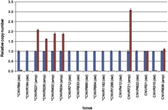
Validation of CNV Segments by qPCR

Twelve singleton CNVRs (asterisks) and six multihit CNVRs were examined by qPCR. Their copy numbers were determined for the samples without copy-number change (blue) or with copy-number change (red). Error bars represent the standard deviation from three determinations. See the text and “Validation of CNV Status by qPCR” in the Material and Methods section. Of the 18 regions examined, copy-number changes were confirmed in 16. See Table S10 for the chromosomal positions of the CNVRs.

Removal of SNP Genotypes in Deletions followed by Sample QC

In comparing SNP and CNVS data, we noticed that genotypes were called for some SNPs in deleted regions. Because the CHMs examined here contained duplicated haploid material, the SNP genotypes called within deletions were likely false. High rates of heterozygous calls of SNPs with a low (< −0.5) log₂ ratio, in contrast to almost entirely homozygous calls for other SNPs, support the conclusion that the majority of the genotypes of the SNPs with low log₂ ratios were false (Figure S3). Therefore, we forced genotypes called at a log₂ ratio less than −0.5 and those within deletions to be “no call.” Approximately 2% of the total SNP calls were rendered “no call” by this filtration step (Figure S1).

Approximately 0.2% of the calls still remained heterozygous, and this could, in principle, be interpreted as evidence that they were in paralogous sequences. The concordance of heterozygous calls for shared SNPs in two comparisons (between Affymetrix SNP Array 6.0 and Affymetrix 500K¹⁵ and between Affymetrix SNP Array 6.0 and Illumina1M-Duo BeadChip), however, were extremely low (1.48% and 2.05%, respectively) (Tables S3 and S4). Therefore, we concluded that error, rather than the presence of paralogous sites, was responsible for the heterozygous calls, and all remaining heterozygous calls were also classified as no calls. After these filtering steps, the call rates of ten CHMs dropped below 95%, and these samples were excluded from further analyses (see Table S1 for QC summary). We also removed one CHM because principal-component analysis revealed that this sample appeared to have exceptionally mixed ancestry and was not suitable as a data source for a typical Japanese population as previously described.¹⁵ As a result of these filtering steps, the call rates of 32,205 SNPs dropped below 85%, and these SNPs were removed (Table S7).

Definitive Haplotype Structures of SNPs and CNVSs

After the refinements described above, the haplotypes of SNPs and CNVSs were definitively delineated on a map containing data from the final 85 CHMs. This map described a total of 875,826 SNPs on autosomes and the X chromosome, 55% of which were 100% called (all 85 CHMs had genotypes) and more than 95% of which were called at least 93% of the time (79 CHMs had genotypes) for the SNPs (Tables S6 and S7).

A total of 6770 CNVSs (4255 deletions and 2515 amplifications) from the 85 CHM samples were included on the map (listed in Table S8). These CNVSs occupied 3.1 Mb per haploid genome (Table S9), in agreement with the previously estimated CNV burden (i.e., equivalent to one half of the value per diploid genome³). Approximately 33% of the CNVSs overlapped with segmental duplications, whereas the overlap was 84% in the combined length of CNVSs, indicating that the CNVSs overlapping with segmental duplications were much larger than those without overlap. The large discrepancy between the means and medians of the segment sizes indicates extreme heterogeneity in the size distribution of the CNVSs (Figure S4), especially for those overlapping with segmental duplications.

CNVRs

CNVRs were defined as mergers of CNVSs across the 85 CHMs and given genome-wide numbers that started at CNVR1, located nearest to the terminus of the short arm of chromosome 1. A total of 1336 CNVRs was identified (listed in Table S10), and 582 of these were mergers of two or more CNVSs (multihit CNVRs) (Table S11). More than half of the CNVRs (754, or 56.4%) were singletons, but singletons accounted for only 11.1% of the detected CNVSs, indicating that most of the CNVSs overlapped with one another.

The fact that there is a greater chance of observing multihit CNVRs (i.e., CNV regions consisting of multiple CNVSs) in regions of segmental duplications known to be preferred sites for nonallelic homologous recombination¹⁸ suggests that many of the multiple hits could be attributable to recurrent ancestral events, not an expansion of the results of single-CNV events in the population.

We compared the CNVRs identified here with previously defined CNPs in a Japanese population (JPT-CNPs) that were also identified with the Affymetrix SNP Array 6.0.³ CNPs have been defined as regions where the copy numbers of included markers tend to vary in a concerted manner among individuals in populations, and they do not overlap with each other.³ The comparison was limited to CNPs and CNVRs on autosomes with an allele frequency of 2% or higher (two or more segments per regions) for both data sets. We also excluded CNVRs that overlapped with segmental duplications from the comparison, because these CNVRs were often very large and spanned regions where markers were very sparse, making precise coverage of the genome ambiguous. With the use of these criteria, approximately 60% of CNPs found in JPT samples overlapped with our CNVRs, accounting for 40% of our CNVRs (Figure 3A).

Figure 3.

Overlap of CNPs with CNVRs or CNVEs

(A) The overlap of CNVRs (red) and CNPs (blue) reported for JPTs³ is shown. CNVRs or CNPs on autosomes that were frequent (> 2%) and nonoverlapping with segmental duplications were compared. Values below are percentages in the respective data sets.

(B) The sizes of overlapping CNVRs and CNPs were compared.

These values for the overlap between CNVRs and CNPs were lower than expected (greater than 90%) if CNPs and CNVRs were present at similar frequencies in both the JPT samples and the CHM samples. Part of the reason for this discrepancy could be explained by differences in the definitions of CNVRs and CNPs. The lower threshold in the definition of CNVRs was based on the number of markers (four or greater) in the regions; thus, some CNVRs were short. On the other hand, many of the candidate short regions were filtered out during QC steps in the CNP definition and were likely underrepresented.³ As a result, approximately 25% of CNVRs were shorter than 2 kb (Figure S4C), whereas less than 8% of CNPs were shorter than that length. It is unknown whether these differences in the definitions explain most of the discrepancies in the overlapping or not.

A comparison of the sizes of CNVRs with Japanese CNPs that overlapped with each other revealed a high correlation, although with some discrepancies (Figure 3B). Essentially all of the CNVRs with sizes greater than an overlapped CNP were found to contain rare (mostly one), large CNVSs that caused an expansion in the size of the CNVRs.

CNV Events

Visual examination of multihit CNVRs revealed that many of them consisted of two or more clusters of CNVSs with different ends and were likely to have resulted from different ancestral events of segmental deletion or amplification. In an attempt to resolve these events, CNV events (CNVEs) were defined as clusters of CNVSs.⁴ Specifically, CNVSs in each CNVR were clustered with the use of a greedy algorithm that consisted of the following steps: (1) groups of CNVSs were determined by their mutual overlap at or above a threshold value; (2) the largest group was identified, and the CNVSs within this group were merged and named a CNVE; (3) the CNVSs belonging to the CNVE were removed, and the procedure was repeated from step 1 until the CNVSs were exhausted. If two or more of the largest groups were found in step 2, the first group identified during the process was adopted. CNVEs were cumulatively numbered, starting from CNVE1 as the first CNVE identified in CNVR1.

By choosing an overlap threshold of 51% of the physical distance, 582 multihit CNVRs were resolved into 1124 CNVEs (listed with allele frequencies in Table S12). Further visual inspection suggested that many of the CNVEs defined here were still heterogeneous and could likely be divided into subevents. We did not attempt to resolve these regions further, due to the difficulty in meaningfully improving event detection because of the extreme bias of marker distribution in or near many CNVRs.

Capturing CNVs by Linkage Disequilibrium with SNPs

We asked how well CNVRs could be captured by linkage disequilibrium with SNP alleles. The examination was limited to common CNVRs (minor allele frequency > 5%) that were deletion changes only and occurred in nonduplicated regions, in order to minimize the effects of possible errors on the definition of CNVSs. As shown in Table 1, approximately one half of the common CNVRs remained uncaptured (maximum r² < 0.8) by SNP markers on SNP Array 6.0.

Table 1.

Capturing CNVRs and CNVEs by SNPs

			Fraction Captureda
Region or Event	Number of Sites	Mean of Max r2	at r2 ≥ 0.5	at r2 ≥ 0.8
CNVRs	130	0.68	0.70	0.49
CNVEs	164	0.59	0.59	0.41

Common deletion CNVRs or CNVEs (frequency ≥ 5%) without segmental duplications were analyzed for linkage disequilibrium with SNPs that were on SNP Array 6.0, located within 200 kb from the boundaries of regions or events with a minor allele frequency ≥ 5%.

^aFractions of CNVRs or CNVEs that were captured by at least one SNP at the indicated r² values.

McCarroll et al. and Cooper et al. have shown that the capture rate of CNV regions by SNPs was approximately half of the rate of SNPs, when the platform Affymetrix SNP Array 6.0 was used.^3,19 They also showed that scarcity of effective SNP markers in the vicinity of CNVRs relative to other genomic regions was the reason for poor capturing of CNVRs. Our observation was in accordance with these earlier reports.

We found that the capture rate (with a maximum r² > 0.8) of amplification CNVRs was lower (0.37) than that of deletion CNVRs (0.47, including those in segmental duplications). An altered physical relationship between CNVRs and adjacent SNPs in samples with amplifications (e.g., due to the location of the amplified copy at a chromosomal position different from original position) is among the possible explanations of the lower capture rate. We also found that deletion CNVRs overlapping with segmental duplications showed a lower capture rate (0.30) in comparison to those in unique regions (0.49), most likely because of the scarcity of SNP markers in segmental duplications.³

Capture rates can also be reduced if the CNVRs are ancestrally heterogeneous; that is, if they consist of two or more CNVEs that occurred independently. In such cases, each of the CNVEs should be more efficiently captured than the CNVRs; however, we found that the capture rate of the CNVEs was consistently low (Table 1). We also defined CNVEs by reciprocal overlap of CNV segments on the basis of the number of markers rather than physical distance, and essentially the same results were obtained (data not shown). These observations are seemingly the opposite of the anticipated results and can be explained if CNVEs within a CNVR have common haplotype backgrounds.

Haplotype Preference of CNVEs

To test the possibility of haplotype sharing between CNVEs, we chose common deletion CNVRs that did not overlap with segmental duplications, consisted of multiple CNVEs, and had at least one common event (allele frequency 5% or higher). We further restricted the comparison by requiring any two CNVEs to be distinguishable by at least two markers and not allowing any of the CNVRs to contain interrupted CNVEs in any of the samples. The rationale for this restriction was to avoid false haplotype similarity caused by erroneous splitting of single events. A total of 35 CNVEs in 17 CNVRs met these criteria. The similarities in haplotype background between common CNVEs within the same CNVR were then examined.

The haplotypes examined here were those defined by SNPs found within 200 kb of both ends of each CNVR. As a measure of haplotype similarity between two CNVEs in a CNVR, we calculated the mean homozygosity of haplotype pairs between every sample in one CNVE and every sample in the other CNVE (observed between-events homozygosity). The tendency of recurrence of the two CNVEs in particular haplotypes was then evaluated against their occurrence in independent haplotypes (which is the expected between-events homozygosity under the assumption of independent occurrence) by bootstrapping the second events. Specifically, the null distribution of homozygosity was generated from 10,000 sets of haplotype pairs with the assumption that the second CNVEs occurred randomly in any of the observed haplotypes of all samples. The probability densities of the null distributions were obtained by kernel-density estimation with the use of R.²⁰ The comparison was limited to 26 cases that gave a unimodal probability density of null distributions as judged by visual inspection. The empirical p value for the occurrence of observed homozygosity in the null distribution was then estimated (see footnote of Table 2).

Table 2.

Haplotype Preference of CNVEs

CNVR	Chr.	First CNVE	Second CNVE	No. of Pairs	Observeda	Nullb	Difference	p Value
CNVR154	2	CNVE228	CNVE227	75	0.7455	0.6151	0.1304	0
CNVR1199	19	CNVE1685	CNVE1684	14	0.8342	0.6704	0.1637	0
CNVR1079	15	CNVE1509	CNVE1508	23	0.8737	0.7079	0.1658	0
CNVR315	4	CNVE432	CNVE431	40	0.8993	0.6347	0.2646	0
CNVR1251	21	CNVE1771	CNVE1770	52	0.9096	0.7458	0.1638	0
CNVR219	3	CNVE304	CNVE303	28	0.9165	0.7028	0.2137	0
CNVR55	1	CNVE103	CNVE102	17	0.9592	0.7225	0.2366	0
CNVR328	4	CNVE448	CNVE449	56	0.7155	0.6316	0.0839	0.0001
CNVR1128	16	CNVE1592	CNVE1591	8	0.8284	0.6387	0.1897	0.0003
CNVR774	10	CNVE1096	CNVE1095	54	0.8332	0.75	0.0833	0.0008
CNVR1251	21	CNVE1770	CNVE1771	52	0.9096	0.7242	0.1854	0.0008
CNVR1251	21	CNVE1772	CNVE1771	4	0.9351	0.7148	0.2203	0.0014
CNVR633	8	CNVE863	CNVE862	56	0.6975	0.6503	0.0472	0.002
CNVR328	4	CNVE449	CNVE448	56	0.7155	0.641	0.0745	0.0039
CNVR774	10	CNVE1095	CNVE1096	54	0.8332	0.747	0.0862	0.006
CNVR154	2	CNVE227	CNVE228	75	0.7455	0.6234	0.1222	0.0111
CNVR592	7	CNVE796	CNVE795	18	0.7494	0.6779	0.0715	0.0115
CNVR1125	16	CNVE1588	CNVE1587	13	0.6877	0.6396	0.0481	0.0157
CNVR633	8	CNVE862	CNVE863	56	0.6975	0.6376	0.06	0.016
CNVR152	2	CNVE225	CNVE224	81	0.6713	0.6324	0.0389	0.0169
CNVR1251	21	CNVE1771	CNVE1772	4	0.9351	0.7464	0.1886	0.0496
CNVR1202	19	CNVE1690	CNVE1689	11	0.777	0.7462	0.0308	0.084
CNVR592	7	CNVE795	CNVE796	18	0.7494	0.6867	0.0628	0.1904
CNVR152	2	CNVE224	CNVE225	81	0.6713	0.6495	0.0219	0.2153
CNVR273	4	CNVE375	CNVE374	18	0.4741	0.5812	−0.1071	0.9962
CNVR649	8	CNVE912	CNVE911	25	0.5285	0.6107	−0.0823	0.9997

^aObserved similarity of haplotype backgrounds between CNVEs in the same CNVR, which was measured by the averaged homozygosity of every between-event haplotype pair.

^bExpected similarity was obtained by bootstrapping to generate null distributions of averaged homozygosity and under the assumption that one of the CNVEs could arise randomly from any of the observed haplotypes. See the text for details regarding the analysis. p values in italics were significant after Bonferroni correction. Additional information on each of the CNVRs and CNVEs is given in Tables S10 and S12.

As shown in Table 2, the means of the homozygosity between events were predominantly higher than the means of the null distributions (24 of 26), and the differences were significant for most comparisons (21 of 26, or 12 of 26 after Bonferroni correction), despite the fact that the number of alleles examined was small. These results indicate that the recurrence of CNVEs is strongly dependent on haplotype. The 12 comparisons that showed strong haplotype similarity were between CNVEs in ten CNVRs, and nine of these CNVRs overlapped with CNPs. The CNVRs carrying CNVEs with significantly similar haplotype backgrounds are shown with the use of the UCSC Genome Browser with modification of some lane names for better visualization (Figure 4 and Figure S5). Figure S6 illustrates the haplotype profiles of CNVE samples and non-CNV samples for all of the CNVRs listed in Table 2 (an example is shown in Figure 5). As is evident from the figure, remarkable haplotype sharing between CNVE samples was evident when compared with non-CNV samples, especially near each of the CNVRs, with one exception (CNVR 273; see Figure S6). In this exceptional CNVR, the two CNVEs seemed to have arisen from different haplotypes.

Figure 4.

Map View of CNVRs Carrying CNVEs with Significant Haplotype Similarity

An example of a CNVR carrying CNVEs with significantly similar haplotype backgrounds is shown with the use of the UCSC Genome Browser. Other examples are presented in Figure S5. Thin bars in orange indicate the positions of CNVSs in individual CHMs. Thick bars in red, black, and blue represent the positions of CNVEs, CNVRs, and CNPs,³ respectively. The bottom two lanes show the positions of SNP markers (Affy 6.0 SNP) and CNV markers (Affy 6.0 SV) in the Affymetrix SNP Array 6.0.

Figure 5.

An Example of Haplotype Sharing between CNVEs

Haplotype profiles of CNVE samples (different CNVEs are color-coded by yellow or green in CNVR lines) and non-CNV samples (black in CNVR lines) for CNVR315 are shown. The major and minor SNP alleles are shown in blue and yellow, respectively, and SNPs with no genotype calls are shown in gray. See Figure S6 for the profiles of other CNVRs listed in Table 2.

Discussion

We determined the haplotype structures of SNPs and CNVSs in Asian genomes, taking advantage of CHMs and their haploid genomes. SNP haplotypes^8,21 and CNV maps^3,4 have been reported previously with the use of HapMap populations; however, the phasing accuracy of the Asian haplotypes has been shown to be more than 10-fold lower than the phasing accuracy for individuals of European descent and Africans.⁹ The high-resolution SNP and CNV definitive haplotype map presented here for a Japanese population is based on the examination of 100 CHMs, which are naturally occurring haploid human samples. Therefore, these haplotypes are definitive, and the phases are accurate.¹⁰

Recent studies have indicated that the maternal physiological state is responsible for mole formation, whereas the sperm genome does not seem to play a role. Thus, the genomes of CHMs can be regarded as unbiased samples of sperm genomes.^22,23 More than 95% of the CHMs studied here were collected within 13 wks of gestation. In such a short period, these CHMs were unlikely to have been subjected to extensive selection. This is in contrast to cultured cell lines, including some HapMap samples known to carry large CNV segments that probably arose during extensive culturing and were fixed by repeated passaging.⁴

CHM genomes have not been biologically proven to be complete in the sense of being capable of supporting the normal development of individuals. Abnormalities that occur de novo in paternal germ cells may remain unselected, so long as the abnormality does not influence cell growth. Such events, however, are likely to be rare.

We genotyped CHMs by using available high-density DNA arrays, and we determined their CNV structures by using a modification of an available method. The copy-number status of each marker in each sample was judged by its signal intensity relative to the intensity of the majority of the samples, which can yield results that differ from the canonical copy-number status (i.e., one copy per haploid), as mentioned earlier. The Canary algorithm²⁴ assigns absolute copy numbers of predefined CNPs for each sample;³ however, this algorithm was developed specifically for diploid samples and could not be directly applied to our haploid samples. Considering this limitation, we analyzed our data by using the Canary analysis module integrated in GTC, assuming that copy numbers of 0 or 1 were deletions and that copy numbers of 3 or 4 were amplifications. As a result, a total of 537 biallelic CNPs were identified, 283 of which overlapped with our biallelic CNVRs. Of these 283 CNPs, 29 were copy-number changes in opposite directions. Thus, approximately 10% of the CNVRs detected were possibly in a copy-number state opposite to the canonical state.

McCarroll et al. defined CNPs as regions where the copy numbers of included markers tend to vary in a concerted manner among individuals in populations.³ By definition, CNPs do not overlap, and many of them seem to behave like biallelic polymorphisms. Recently, however, many CNPs have been shown to be resolvable to several different ancestral events.^25,26 Therefore, we attempted to resolve CNVRs into CNVEs by reciprocal overlaps of CNVSs. The resolution was far from perfect, and many of the CNVEs seemed to consist of subevents; however, different origins of ancestral events were evident between different CNVEs.

Comparisons of surrounding haplotypes between CNVEs belonging to the same CNVR revealed that most of the haplotypes were significantly similar. One plausible explanation for this is that the presence of CNVSs induces instability in the region and encourages secondary amplifications or deletions within the same allele, although other explanations are also possible. Although this scenario sounds like a remote possibility, it may not be if one considers the situation of CNVSs in meiosis. During meiosis, CNVSs are almost always paired with normal counterparts (given their low allele frequencies, at least when they are newly formed), and the local instability caused by imperfect asymmetric homologous paring of chromatids may render these sites or their vicinity vulnerable to secondary events such as amplifications or deletions.

The similarity of the haplotype backgrounds between CNVEs in the same CNVR has been implicated, although not explicitly stated, in previous reports.³ McCarroll et al. demonstrated that most CNPs could be captured at a high linkage disequilibrium by nearby SNPs if the SNPs used were of sufficiently high density to allow estimation of the capture rate, despite the fact that some of the CNPs were clusters of CNVEs. These findings are most easily understood if haplotype-dependent recurrence of CNVEs is assumed. The possible dependence of CNVE occurrence on preexisting events is in contrast to SNPs, which can be regarded as the result of independent, random events.

The determination of CNV structure with the use of available arrays involves some uncertainty because of the extremely uneven distribution of markers, as noted previously.^3,19 Perhaps significant improvement in the detection of CNVs must await the availability of arrays carrying an unbiased distribution of markers. Recently, Conrad et al. reported an advanced CNV-typing array system that can efficiently detect even small CNVs.²⁷ With the use of this system, the detection of CNVs in existing materials should be improved; however, this system still suffers from the fact that detecting CNVs in the Asian genome is highly inefficient (the number of CNVs detectable in Asians is approximately two-thirds that of individuals of European descent). This is because the initial experiments conducted to determine the markers to be loaded in the typing arrays were carried out with the use of European-descent and African samples, resulting in some population bias in the detection efficiency of the typing array.

Non-hybridization-based methods such as resequencing by new-generation sequencers are obviously among other future approaches. CHM samples provide an exceptional opportunity for effective whole-genome resequencing because CHMs display genome-wide homozygosity and require less sequencing redundancy. Furthermore, the reads can be aligned with greater confidence, unlike resequencing of diploid materials.

Web Resources

The URLs for the data and software used herein are as follows:

• Affymetrix: Genotyping Console software and annotation files, http://www.affymetrix.com/

• Database of Genomic Variants, http://projects.tcag.ca/variation

• dbSNP, http://www.ncbi.nlm.nih.gov/projects/SNP/

• Illumina: BeadStudio software and other requirement files, http://www.illumina.com/

• R software, http://www.R-project.org

• UCSC Genome Browser: genome annotation and SNP array marker information, http://genome.ucsc.edu/

Accession Numbers

The Gene Expression Omnibus (GEO) accession number for the array intensity data reported in this paper is GSE18701.

References

- 1.Iafrate A.J., Feuk L., Rivera M.N., Listewnik M.L., Donahoe P.K., Qi Y., Scherer S.W., Lee C. Detection of large-scale variation in the human genome. Nat. Genet. 2004;36:949–951. doi: 10.1038/ng1416. [DOI] [PubMed] [Google Scholar]
- 2.Sebat J., Lakshmi B., Troge J., Alexander J., Young J., Lundin P., Månér S., Massa H., Walker M., Chi M. Large-scale copy number polymorphism in the human genome. Science. 2004;305:525–528. doi: 10.1126/science.1098918. [DOI] [PubMed] [Google Scholar]
- 3.McCarroll S.A., Kuruvilla F.G., Korn J.M., Cawley S., Nemesh J., Wysoker A., Shapero M.H., de Bakker P.I., Maller J.B., Kirby A. Integrated detection and population-genetic analysis of SNPs and copy number variation. Nat. Genet. 2008;40:1166–1174. doi: 10.1038/ng.238. [DOI] [PubMed] [Google Scholar]
- 4.Redon R., Ishikawa S., Fitch K.R., Feuk L., Perry G.H., Andrews T.D., Fiegler H., Shapero M.H., Carson A.R., Chen W. Global variation in copy number in the human genome. Nature. 2006;444:444–454. doi: 10.1038/nature05329. [DOI] [PMC free article] [PubMed] [Google Scholar]
- 5.Feuk L., Marshall C.R., Wintle R.F., Scherer S.W. Structural variants: changing the landscape of chromosomes and design of disease studies. Hum. Mol. Genet. 2006;15(Spec No 1):R57–R66. doi: 10.1093/hmg/ddl057. [DOI] [PubMed] [Google Scholar]
- 6.McCarroll S.A. Extending genome-wide association studies to copy-number variation. Hum. Mol. Genet. 2008;17(R2):R135–R142. doi: 10.1093/hmg/ddn282. [DOI] [PubMed] [Google Scholar]
- 7.Cook E.H., Jr., Scherer S.W. Copy-number variations associated with neuropsychiatric conditions. Nature. 2008;455:919–923. doi: 10.1038/nature07458. [DOI] [PubMed] [Google Scholar]
- 8.Frazer K.A., Ballinger D.G., Cox D.R., Hinds D.A., Stuve L.L., Gibbs R.A., Belmont J.W., Boudreau A., Hardenbol P., Leal S.M., International HapMap Consortium A second generation human haplotype map of over 3.1 million SNPs. Nature. 2007;449:851–861. doi: 10.1038/nature06258. [DOI] [PMC free article] [PubMed] [Google Scholar]
- 9.Kidd J.M., Cheng Z., Graves T., Fulton B., Wilson R.K., Eichler E.E. Haplotype sorting using human fosmid clone end-sequence pairs. Genome Res. 2008;18:2016–2023. doi: 10.1101/gr.081786.108. [DOI] [PMC free article] [PubMed] [Google Scholar]
- 10.Kukita Y., Miyatake K., Stokowski R., Hinds D., Higasa K., Wake N., Hirakawa T., Kato H., Matsuda T., Pant K. Genome-wide definitive haplotypes determined using a collection of complete hydatidiform moles. Genome Res. 2005;15:1511–1518. doi: 10.1101/gr.4371105. [DOI] [PMC free article] [PubMed] [Google Scholar]
- 11.Peiffer D.A., Le J.M., Steemers F.J., Chang W., Jenniges T., Garcia F., Haden K., Li J., Shaw C.A., Belmont J. High-resolution genomic profiling of chromosomal aberrations using Infinium whole-genome genotyping. Genome Res. 2006;16:1136–1148. doi: 10.1101/gr.5402306. [DOI] [PMC free article] [PubMed] [Google Scholar]
- 12.Rozen S., Skaletsky H.J. Primer3 on the WWW for general users and for biologist programmers. In: Krawetz S., Misener S., editors. Bioinformatics Methods and Protocols: Methods in Molecular Biology. Humana Press; Totowa, NJ: 2000. pp. 365–386. [DOI] [PubMed] [Google Scholar]
- 13.Wang T.L., Maierhofer C., Speicher M.R., Lengauer C., Vogelstein B., Kinzler K.W., Velculescu V.E. Digital karyotyping. Proc. Natl. Acad. Sci. USA. 2002;99:16156–16161. doi: 10.1073/pnas.202610899. [DOI] [PMC free article] [PubMed] [Google Scholar]
- 14.Livak K.J., Schmittgen T.D. Analysis of relative gene expression data using real-time quantitative PCR and the 2(-Delta Delta C(T)) method. Methods. 2001;25:402–408. doi: 10.1006/meth.2001.1262. [DOI] [PubMed] [Google Scholar]
- 15.Higasa K., Kukita Y., Kato K., Wake N., Tahira T., Hayashi K. Evaluation of haplotype inference using definitive haplotype data obtained from complete hydatidiform moles, and its significance for the analyses of positively selected regions. PLoS Genet. 2009;5:e1000468. doi: 10.1371/journal.pgen.1000468. [DOI] [PMC free article] [PubMed] [Google Scholar]
- 16.Zhang J., Feuk L., Duggan G.E., Khaja R., Scherer S.W. Development of bioinformatics resources for display and analysis of copy number and other structural variants in the human genome. Cytogenet. Genome Res. 2006;115:205–214. doi: 10.1159/000095916. [DOI] [PubMed] [Google Scholar]
- 17.Bailey J.A., Yavor A.M., Massa H.F., Trask B.J., Eichler E.E. Segmental duplications: organization and impact within the current human genome project assembly. Genome Res. 2001;11:1005–1017. doi: 10.1101/gr.187101. [DOI] [PMC free article] [PubMed] [Google Scholar]
- 18.Sharp A.J., Locke D.P., McGrath S.D., Cheng Z., Bailey J.A., Vallente R.U., Pertz L.M., Clark R.A., Schwartz S., Segraves R. Segmental duplications and copy-number variation in the human genome. Am. J. Hum. Genet. 2005;77:78–88. doi: 10.1086/431652. [DOI] [PMC free article] [PubMed] [Google Scholar]
- 19.Cooper G.M., Zerr T., Kidd J.M., Eichler E.E., Nickerson D.A. Systematic assessment of copy number variant detection via genome-wide SNP genotyping. Nat. Genet. 2008;40:1199–1203. doi: 10.1038/ng.236. [DOI] [PMC free article] [PubMed] [Google Scholar]
- 20.R Development Core Team . R Foundation for Statistical Computing; Vienna, Austria: 2008. R: A language and environment for statistical computing. [Google Scholar]
- 21.International HapMap Consortium A haplotype map of the human genome. Nature. 2005;437:1299–1320. doi: 10.1038/nature04226. [DOI] [PMC free article] [PubMed] [Google Scholar]
- 22.Murdoch S., Djuric U., Mazhar B., Seoud M., Khan R., Kuick R., Bagga R., Kircheisen R., Ao A., Ratti B. Mutations in NALP7 cause recurrent hydatidiform moles and reproductive wastage in humans. Nat. Genet. 2006;38:300–302. doi: 10.1038/ng1740. [DOI] [PubMed] [Google Scholar]
- 23.Slim R., Mehio A. The genetics of hydatidiform moles: new lights on an ancient disease. Clin. Genet. 2007;71:25–34. doi: 10.1111/j.1399-0004.2006.00697.x. [DOI] [PubMed] [Google Scholar]
- 24.Korn J.M., Kuruvilla F.G., McCarroll S.A., Wysoker A., Nemesh J., Cawley S., Hubbell E., Veitch J., Collins P.J., Darvishi K. Integrated genotype calling and association analysis of SNPs, common copy number polymorphisms and rare CNVs. Nat. Genet. 2008;40:1253–1260. doi: 10.1038/ng.237. [DOI] [PMC free article] [PubMed] [Google Scholar]
- 25.Perry G.H., Ben-Dor A., Tsalenko A., Sampas N., Rodriguez-Revenga L., Tran C.W., Scheffer A., Steinfeld I., Tsang P., Yamada N.A. The fine-scale and complex architecture of human copy-number variation. Am. J. Hum. Genet. 2008;82:685–695. doi: 10.1016/j.ajhg.2007.12.010. [DOI] [PMC free article] [PubMed] [Google Scholar]
- 26.Pique-Regi R., Ortega A., Asgharzadeh S. Joint estimation of copy number variation and reference intensities on multiple DNA arrays using GADA. Bioinformatics. 2009;25:1223–1230. doi: 10.1093/bioinformatics/btp119. [DOI] [PMC free article] [PubMed] [Google Scholar]
- 27.Conrad D.F., Pinto D., Redon R., Feuk L., Gokcumen O., Zhang Y., Aerts J., Andrews T.D., Barnes C., Campbell P., Wellcome Trust Case Control Consortium Origins and functional impact of copy number variation in the human genome. Nature. 2010;464:704–712. doi: 10.1038/nature08516. [DOI] [PMC free article] [PubMed] [Google Scholar]
Associated Data
This section collects any data citations, data availability statements, or supplementary materials included in this article.