Implementation and Evaluation of the SAEM Algorithm for Longitudinal Ordered Categorical Data with an Illustration in Pharmacokinetics–Pharmacodynamics

Abstract

Analysis of longitudinal ordered categorical efficacy or safety data in clinical trials using mixed models is increasingly performed. However, algorithms available for maximum likelihood estimation using an approximation of the likelihood integral, including LAPLACE approach, may give rise to biased parameter estimates. The SAEM algorithm is an efficient and powerful tool in the analysis of continuous/count mixed models. The aim of this study was to implement and investigate the performance of the SAEM algorithm for longitudinal categorical data. The SAEM algorithm is extended for parameter estimation in ordered categorical mixed models together with an estimation of the Fisher information matrix and the likelihood. We used Monte Carlo simulations using previously published scenarios evaluated with NONMEM. Accuracy and precision in parameter estimation and standard error estimates were assessed in terms of relative bias and root mean square error. This algorithm was illustrated on the simultaneous analysis of pharmacokinetic and discretized efficacy data obtained after a single dose of warfarin in healthy volunteers. The new SAEM algorithm is implemented in MONOLIX 3.1 for discrete mixed models. The analyses show that for parameter estimation, the relative bias is low for both fixed effects and variance components in all models studied. Estimated and empirical standard errors are similar. The warfarin example illustrates how simple and rapid it is to analyze simultaneously continuous and discrete data with MONOLIX 3.1. The SAEM algorithm is extended for analysis of longitudinal categorical data. It provides accurate estimates parameters and standard errors. The estimation is fast and stable.

INTRODUCTION

Mixed effect analyses are increasingly employed for the analysis of longitudinal efficacy or safety categorical data measured in clinical trials (1–5). For this purpose, proportional odds model are frequently used. Other models, such as differential odds model, have also been proposed (6). Results from these analyses, i.e., models along with parameter estimates, are often further utilized for simulation of novel scenarios with respect to new dosing schedules or new patient populations. It is also advocated that these models should be used as an essential part of drug development programs. Therefore, it is critical that these parameter estimates are unbiased and reliable.

We focus here on maximum likelihood estimation. However, as in all nonlinear mixed models, the integral of the likelihood function cannot be explicitly solved, and various approximations are employed to approximate the true likelihood (7). The most commonly used approximation is LAPLACE, available in the software NONMEM. Bias in parameter estimates for these models with NONMEM VI and SAS v.8 has been studied in detail, and it has been shown that the use of LAPLACE approximation may result in severely biased estimates, especially when response categories are non-evenly distributed within the studied population (8). This is common when analyzing clinical data, and therefore, the importance of using exact evaluations of the likelihood integral is further accentuated.

SAS implements a more exact evaluation of the likelihood using adaptive Gaussian quadrature. However, this approach is time consuming, can be applied to models with limited number of random effects, and is not flexible for the analysis of pharmacokinetic/pharmacodynamic data after various repeated dosage regimen (9).

In recent years, there have been several approaches/algorithms developed for the analysis of continuous data, which are able to find maximum likelihood estimates without a need to compute the likelihood numerically (10,11). A stochastic approximation version of EM algorithm linked to a Markov Chain Monte Carlo procedure has been suggested for maximum likelihood estimation within the non-linear mixed effects framework (11,12). This procedure has been demonstrated to possess excellent statistical convergence properties as well as the ability to provide an estimator close to the maximum likelihood estimate in only a few iterations (12,13). In addition to the estimation of the maximum likelihood parameters, the SAEM algorithm also provides the user with the estimate of the Fisher information matrix, used to assess parameter estimate uncertainty. However, there have been no studies reported with respect to application of the stochastic algorithms to the analysis of the ordered categorical data.

The aims of this study were (1) to extend the SAEM algorithm for estimation of parameters in categorical data mixed models, (2) to evaluate its performance both for parameter and standard errors estimation via Monte Carlo simulation study, and (3) to illustrate the performance of the algorithm on a real data example where both continuous pharmacokinetic (PK) and discrete pharmacodynamic (PD) data are simultaneously analyzed.

A proportional odds model with individual-specific random effect has been employed throughout the exercise to study properties of the new SAEM algorithm. This model has been used in the area of PKPD modeling (2,5,14) and has been presented in detail elsewhere (2,5,8,14).

METHODS

The Proportional Odds Model with Random Intercept

We assume that the response is an ordered categorical variable which takes its values in (0,1,…,M). Let y_ij be the jth observation in the ith individual, i = 1, …, N. In the proportional odds model with random intercept, the cumulative probability of y_ij being larger or equal to m (m = 1, …, M), can be defined by the following logistic regression model

1

where logit denotes the logit function, α₁ +... + α_m specifies the baseline for category m (m = 1, …, M), h is the function defining predictors or covariate effect, β is a vector of fixed effects which is the same across all categories, x_ijis the predictor vector (e.g., time, dose, concentration, etc) for observation j of individual i, and η_i is the random effect of individual i. It is assumed that the random effects are normally distributed with mean 0 and variance ω².

Implementation of the SAEM Algorithm for Categorical Data Models

The SAEM algorithm as described in Kuhn and Lavielle (11) for continuous data models has been extended to the ordered categorical data models in a similar manner as it has been done for the count data models (13). Let μ = (α₁,α₂,...,α_M,β₁,β₂...β_L) be the vector of fixed effects of the model and Ω be the variance–covariance matrix of the random effects η_i (in our example, ω_i is scalar, and Ω reduces to the variance ω² of η_i). Then, SAEM is an iterative procedure where at iteration k, a new set of random effects η^(k) = (η_i^(k)) is drawn with the conditional distribution p(η|y; μ^(k), Ω^(k)). Then, the new population parameters (μ^(k + 1), Ω^(k + 1)) are obtained by maximizing Q_k + 1(μ, Ω) defined as follows:

2

where l(y, η; μ, Ω) is the complete log-likelihood

3

and where (γ_k) is a decreasing sequence of step sizes. For the numerical experiments presented below, we used γ_k = 1 during the first 200 iterations of SAEM and γ_k = 1/(k − 200) during the next 100 iterations.

An MCMC algorithm was used for the simulation step (see Kuhn and Lavielle (11) and Lavielle and Mentre (12) for more details).

Estimation of the Fisher Information Matrix

Let θ = (μ, Ω) be the set of population parameters to be estimated, and let be the maximum likelihood estimate of θ computed with SAEM. The Fisher information matrix is defined as , where is the log-likelihood of the observations, computed with .

Several numerical experiments have shown that linearization of the model for estimating the Fisher information matrix (as implemented in MONOLIX 2.4) is satisfactory in case of continuous data (15).

In this case, the linearization of the structural model allows the transformation of the non-linear model into a Gaussian model, in which the Fisher information matrix can be computed in a closed form.

However, this approach cannot be applied for discrete data models. As alternative, we propose to compute a stochastic approximation of the Fisher information matrix using the Louis formula (see Kuhn and Lavielle (11) for more details):

4

The procedure consists in computing first with SAEM then applying the Louis formula with , which requires the computation of the conditional expectation and conditional variance defined in Eq. 4. These quantities are estimated by Monte Carlo: 300 iterations of MCMC were performed for the numerical experiments. All extensions for SAEM algorithm described here have been implemented in software MONOLIX 3.1.

Simulation Settings

The performance of the SAEM algorithm was evaluated via Monte Carlo simulation. To allow a fair comparison with other algorithms, we used identical scenarios as presented previously in the paper of Jönsson et al. where authors explored performance of LAPLACE and adaptive Gaussian quadrature algorithms (8). Overall, five different scenarios (A–E) were used. In all scenarios, response was a four-level categorical variable that takes its values in {0,1, 2,3}. Scenarios A–C describe a baseline model

5

with three different distributions of response categories: even (scenario A), moderately skewed (scenario B) and skewed (scenario C).

Scenario D–E included a specific baseline, placebo, and drug model through two additional β parameters Eq. 6

6

The placebo model was implemented as a step function (c_ij = 0 if j = 1 and c_ij = 1 if j = 2,3,4), while the drug model was implemented as a linear function of the dose (d_ij = 0 if j = 1 and d_ij = 7.5,15,30 if j = 1,2,3,4) respectively. The distribution of response categories was even (scenario D) and skewed (scenario E).

Typical parameter values were chosen so as to mimic desired distribution of responses. The studied variance range was 0.5–40.

For each scenario, 100 datasets each containing 1000 individuals were simulated with MATLAB. All estimation procedures were performed using MONOLIX 3.1.

Overview of studied scenarios is shown in Table I. For more details on the simulation design used, the reader is kindly asked to refer to the original publication of Jönsson et al. (8).

Table I.

Original Study Design and Simulation Settings

Scenario	α 1	α 2	α 3	β 1	β 2	ω 2	Proportions 0:1:2:3 (%)
A (baseline)	1.85	−1.85	−1.85	–	–	4	25:25:25:25
	2.47	−2.46	−2.42	–	–	10
	4.46	−4.44	−4.41	–	–	40
B (baseline)	−2.45	−1.375	−1.50	–	–	4	82.5:10:5:2.5
	−3.34	−1.84	−1.99	–	–	10
	−6.02	−3.28	−3.55	–	–	40
C (baseline)	−2.383	−0.775	−0.965	–	–	0.5	90:5:3:2
	−2.865	−0.877	−1.05	–	–	2
	−3.39	−1.01	−1.19	–	–	4
	−4.59	−1.35	−1.58	–	–	10
	−8.25	−2.43	−2.86	–	–	40
D (baseline placebo + drug)	1.85	−1.85	−1.85	0.483	0.046	4	25:25:25:25
E (baseline placebo + drug)	−3.538	−0.447	−1.02	1.318	0.024	0.5	96.5:1.2:1.4:0.9
	−4.882	−0.548	−1.183	1.548	0.030	4
	−11.815	−1.322	−2.962	3.851	0.072	40

Distribution of response categories for originally simulated data sets and true parameter values used in simulations are presented

Evaluation of the SAEM Algorithm and the Standard Error Estimates

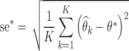
For each scenario, the SAEM algorithm was used with the K = 100 simulated datasets for computing the K parameter estimates, . The Fisher information matrix was also estimated for each data set, and its inverse was used to compute the K standard error estimates, . The empirical standard errors se* (i.e. the RMSE) were computed by Eq. 7:

7

where θ^* stands for the true parameter value.

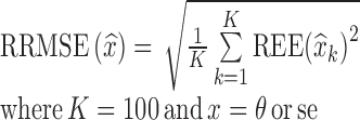
To assess statistical properties of the proposed estimators, for each parameter, relative estimation errors were computed as shown in Eq. 8a, where x_k = θ_k. Similarly, for each estimated parameter standard error, relative estimation error was computed, as shown in Eq. 8a, where x = se. Each relative estimation error (REE) is expressed as a percentage. From the REEs, relative bias (RB) and relative root mean square errors (RRMSE) were computed for each parameter in each scenario as shown in Eqs. 8b and 8c.

8a

8b

8c

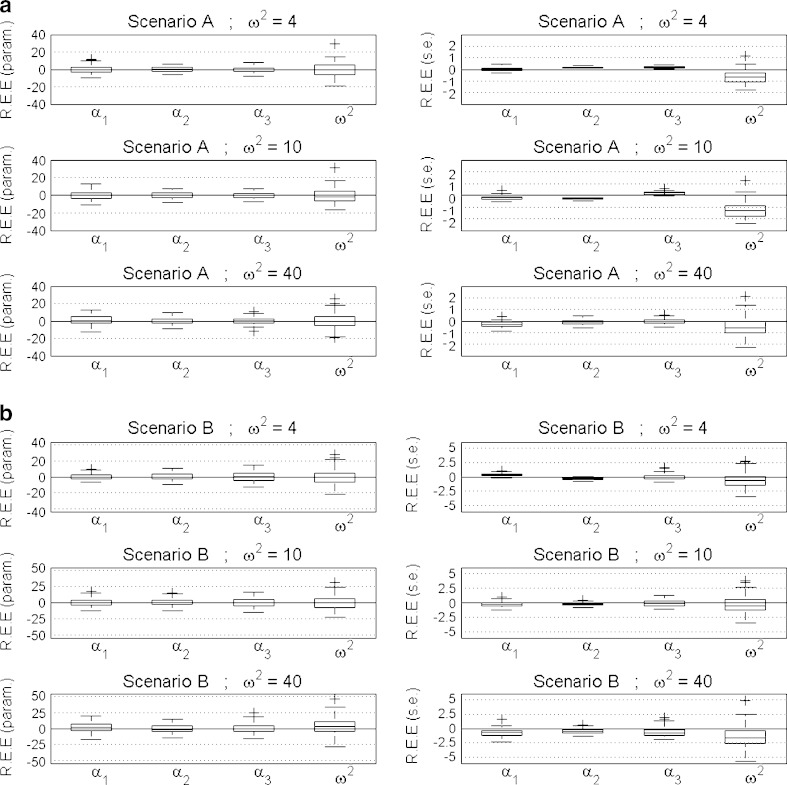
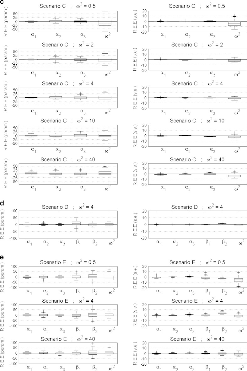
For simplicity in the notations, all these formulas are vectorial formula, which holds for each component of θ. Outcomes of all Monte Carlo simulation studies exploring both the parameter estimation procedure and estimation of Fisher information matrix were presented as box plots of REEs where bias and imprecision of the method, as defined by Eqs. 8b and 8c, can easily be visualized.

Central processing unit (CPU) times needed for estimation of (a) population parameters, (b) empirical Bayes estimates (EBEs), which are individual random effects, and (c) standard error estimates, were also measured to assess the efficiency of the algorithm and the runtime for the analysis.

Illustration on Real Data

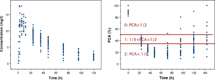
The well-known real PKPD dataset of warfarin was used to evaluate novel SAEM algorithm and its ability to simultaneously analyze continuous and categorical data. The data were collected in 33 patients after a single dose of warfarin for 140 h post dose. In total, 251 PK observations and 232 PD observations (corresponds to inhibition of prothrombin complex synthesis—PCA (%)) were available (16,17). Original PD variable was continuous variable expressed in percentages (0–100%); however, for our purpose, we categorized the PCA variable into three ordered categories: 0 (if PCA is more than 50%), 1 (if PCA is between 33% and 50%), and 2 (if PCA was less than 33%). Of note, categorization of the continuous variable is done for illustration purpose only, and it is not recommended to be done in the real analysis. The cutoffs chosen are close to international normalized ration (INR) values commonly used in clinical practice to target optimal warfarin therapy. Low INR values (<2) are associated with high risk of having a cloth (corresponding to category 0), high INR values (>3) with high risk of bleeding (corresponding to category 2), while targeted value of INR, corresponding to optimal therapy is in between 2 and 3 (corresponding to category 1). The raw PKPD data are shown in Fig. 1. The PK model fitted was one compartment model with first-order absorption and a lag time. Effect compartment model was used to mimic an effect delay. Proportional odds model with random intercept was used to fit ordered categorical response. The drug model was a linear function of warfarin concentration.

Fig. 1.

Observed pharmacokinetic (left panel) and pharmacodynamic (right panel) data of warfarin. The categorization of the continuous PD variable (PCA) is visualized with the horizontal lines representing cut-off values

RESULTS

Simulation Study

Overall, the estimation procedure with the SAEM algorithm for mixed categorical data models showed satisfactory performance with low bias and high precision. Convergence was 100% for both parameter and standard error estimation. For parameter estimation, the absolute value of relative bias was less than 7.9% and 8.13% for fixed effects, and the random effect variances and RRMSE was less than 27% and 30% for fixed effects and the random effect variances overall tested scenarios. For standard error estimation, the absolute value of relative bias was less than 3.4% and 5.8% for fixed effects and random effect variances, and RRMSE was less than 2.3% and 5.6% for fixed effects and random effect variances. The random effect variances, shown to be severely biased when estimated with LAPLACE method implemented in NONMEM (8), were precisely estimated with SAEM, exhibiting relative bias ranging from 0.03% to 8.13% across all studied scenarios. Detailed results for each scenario are listed below. The distribution of REE for all scenarios and all parameter and standard error estimates are shown in Fig. 2a–e. The numerical results showing accuracy and precision for parameter estimation, measured as relative bias and relative root mean square error, are shown in Table II. The numerical results showing accuracy and precision for relative standard error estimation, measured as bias and root mean square error, are shown in Table III, indicating low bias (<5.78%) and high precision (RRMSE < 7.42%).

Fig. 2.

a–e Distribution of relative estimation error (REE) for all parameters (left panel) and standard errors (right panel) across all the models. The errors (y-axes) are given as percentages

Table II.

Relative Bias and Relative Root Mean Square Error (in %) for Parameter Estimates for All Studied Scenarios

Simulation		Parameter estimates			Relative bias (%)
					Relative RMSE (%)
Scenario	ω 2	α 1	α 2	α 3	β 1	β 2	ω 2
A	4	−0.30	−0.09	−0.43	–	–	−0.11
		4.45	2.88	2.82	–	–	7.89
	10	−0.08	−0.23	−0.08	–	–	−0.23
		5.14	3.36	5.14	–	–	3.36
	40	0.69	−0.12	0.41	–	–	−0.03
		5.78	3.71	3.68	–	–	8.11
B	4	0.11	0.20	0.26	–	–	−0.42
		4.10	5.29	6.99	–	–	11.39
	10	0.18	0.54	−0.47	–	–	0.12
		5.53	5.22	7.01	–	–	10.82
	40	1.63	−0.03	0.49	–	–	3.01
		7.41	5.80	8.03	–	–	13.29
C	0.5	−0.21	1.15	−2.46	–	–	−8.13
		3.00	7.25	9.27	–	–	30.34
	2	−0.59	0.86	−0.49	–	–	−3.41
		3.75	7.78	8.43	–	–	16.79
	4	−0.04	1.29	−0.84	–	–	−0.44
		4.24	7.48	9.76	–	–	14.39
	10	1.28	0.43	0.49	–	–	3.18
		5.56	6.38	10.10	–	–	14.45
	40	2.04	1.54	1.11	–	–	4.94
		7.93	7.86	9.39	–	–	17.68
D	4	−0.08	0.66	0.70	7.95	−0.84	1.16
		5.41	3.23	3.34	20.83	10.46	8.13
E	0.5	−2.05	−1.31	−1.16	0.11	5.52	−7.46
		5.77	7.99	6.64	14.75	23.37	29.82
	4	−0.21	−0.94	0.79	−2.74	2.62	2.40
		5.66	9.72	6.75	14.98	24.06	14.64
	40	0.84	2.73	−0.44	−1.91	6.93	3.73
		6.90	9.27	7.77	10.86	27.45	15.95

These results correspond to the visual ones shown in the left panel of Fig. 2a–e

Table III.

Relative Bias and Relative Root Mean Square Error (in %) for Standard Error Estimates for All Studied Scenarios

Simulation		Standard error estimates			Relative bias (%)
					Relative RMSE (%)
Scenario	ω 2	se(α 1)	se(α 2)	se(α 3)	se(β 1)	se(β 2)	se(ω 2)
A	4	0.00	0.13	0.18	–	–	−0.67
		0.14	0.15	0.20	–	–	0.87
	10	−0.23	−0.25	0.17	–	–	−1.28
		0.30	0.27	0.20	–	–	1.43
	40	−0.30	−0.10	−0.02	–	–	−0.51
		0.39	0.24	0.19	–	–	0.93
B	4	0.35	−0.36	0.01	–	–	−0.69
		0.44	0.42	0.46	–	–	1.39
	10	−0.29	−0.26	−0.10	–	–	−0.40
		0.49	0.36	0.49	–	–	1.40
	40	−0.73	−0.53	−0.61	–	–	−1.56
		0.96	0.66	1.01	–	–	2.34
C	0.5	−0.17	−0.12	−0.09	–	–	−4.19
		0.43	0.37	0.69	–	–	6.98
	2	0.02	−0.73	0.70	–	–	−2.03
		0.35	0.82	0.98	–	–	3.06
	4	0.01	−0.46	−0.77	–	–	−1.56
		0.32	0.59	1.1	–	–	2.19
	10	−0.50	0.52	−1.23	–	–	−2.01
		0.68	0.66	1.43	–	–	2.76
	40	−1.58	−0.91	−0.28	–	–	−4.27
		1.73	1.09	1.01	–	–	4.99
D	4	−0.02	0.06	−0.36	−0.08	1.27	−0.79
		0.14	0.11	0.37	0.28	1.29	0.97
E	0.5	−1.69	−0.03	0.33	−1.79	−2.48	−5.78
		1.91	0.39	0.51	2.62	2.61	7.42
	4	−0.73	−1.06	0.64	−0.11	3.37	−1.73
		0.89	1.18	0.77	0.99	3.64	2.52
	40	−1.27	−0.63	−0.36	−0.35	−0.43	−2.36
		1.43	0.84	0.66	1.09	2.35	3.39

These results correspond to the visual ones shown in the right panel of Fig. 2a–e

The average CPU time per run over all scenarios was 29.6 s for parameter estimation and 6.5 s for standard error estimation, with Matlab/C++ implementation of the algorithm, when ran on laptop DELL D830 2.40 GHz configuration. Median CPU times for parameter, EBEs, and standard error estimation are given in Table IV, for all studied scenarios.

Table IV.

Median CPU Time for Parameter, EBE, and Standard Error Estimations for All Studied Scenarios

Scenario	ω 2	Median CPU time (s)a
		Parameters	EBE	Standard errors
A	4	29.3	12.0	5.2
	40	27.9	11.2	5.1
B	4	28.5	11.4	5.4
	40	29.0	11.0	5.1
C	0.5	28.6	11.2	5.5
	40	28.7	11.4	5.2
D	4	30.8	7.4	8.4
E	0.5	33.1	7.8	8.2
	4	30.1	9.5	8.3
	40	30.0	11.4	8.2

^aLaptop DELL D830 2.40 GHz configuration was used with Matlab/C++ implementation of SAEM

Illustration on Real Data

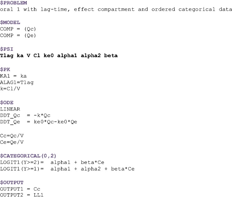
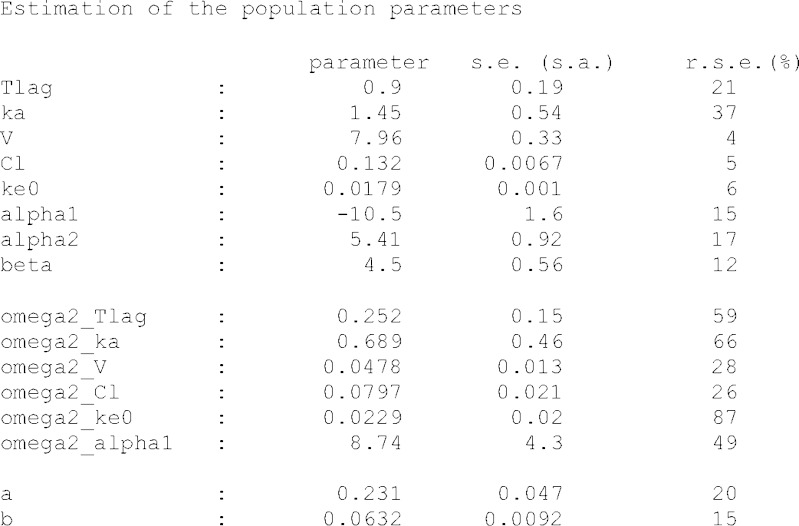
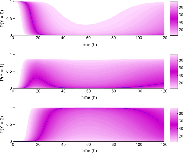
With respect to the warfarin real data example, both parameter and standard error estimation were successful. Estimation procedure was completed in less than 2 min, for the model containing eight typical parameters, six variances, and two residual error parameters. The example of the model implementation in MONOLIX 3.1 is shown in Fig. 3. The output of MONOLIX run representing parameter estimates and respective standard errors is shown in Fig. 4. Figure 5 shows change over time of probability of each response category, based on the simulations from the final model.

Fig. 3.

Implementation of the simultaneous analysis of continuous and discrete data in MONOLIX for the warfarin dataset. Pharmacokinetics is described with one compartment model with first-order absorption and a lag time. Effect compartment model is used to mimic the effect delay. Proportional odds model is used to fit ordered categorical PD variable

Fig. 4.

MONOLIX output for real data example. Parameter estimates are shown along with their standard error estimates

Fig. 5.

Predicted probability over time for each warfarin response category (0, 1, and 2 for the upper, middle, and lower panel, respectively), based on the simulations from the final model. The simulated median (50th percentile) is shown in blue, while range of prediction intervals around the median are shown in a different shade of pink according to the color scale of percentiles shown to the right

DISCUSSION

The new SAEM algorithm has been developed, implemented, and evaluated for application to categorical data models in the non-linear mixed effects framework. Five different scenarios using proportional odds model were evaluated, including those with non-even distribution of response categories. The algorithm was also implemented for computation of Fisher information matrix in order to assess the uncertainty estimate.

The SAEM algorithm performed well under all tested model scenarios resulting in accurate and precise estimation of all parameters. Variances of scenarios with non-even distribution of response categories were accurately and precisely estimated, which was not reported previously in analysis with the LAPLACE method (8). The explanation for previously observed biases with LAPLACE was related to the poor approximation of the likelihood integral. Similar to FOCE (first-order approximation), LAPLACE approximation involves linearization of the function by means of estimating EBE at each iteration step in order to approximate likelihood. Therefore, whenever data are sparse, which may be due to design, variability, or the model itself, shrinkage in EBE leads to linearization around zero for the random effects, close to an FO method, which is known to be biased (18,19). Additionally, random effects enter models in a non-linear fashion; therefore, these are most likely to suffer from the poor integral approximation, which was indeed observed in the previous work with severely biased variances (8). Gaussian quadrature method, as implemented in SAS, performed better than LAPLACE due to better numerical approximation of the likelihood integral; therefore, EBE shrinkage influence was less pronounced compared with the LAPLACE approximation (8). Similar pattern was also observed when performance of these estimation methods was evaluated for count data (13,20). Of note, it has been reported that this Gaussian quadrature may become unstable and time consuming for more complex type of problems (7,21).

The SAEM algorithm does not involve any likelihood estimation conditioned on EBEs or any approximation of the model in computation of the likelihood integral and therefore does not suffer from any related biases. SAEM during minimization procedure compute the full conditional distribution of the individual parameters and simulate large number of individual parameters using these conditional distributions at the current iteration—these will have large variability in case of sparse individual information, and EBE shrinkage is not a problem under these circumstances. Of note, small significant bias was observed in scenario D for estimation of β₁ parameter, which is magnitude of treatment effect. This bias is most likely related to the small number of observations per subject as it disappeared when the number of observations per subject was increased.

The SAEM algorithm provides estimation of both the likelihood and Fisher information matrix, without linearization of the model. This is a favorable property of the algorithm, which leads to accurate and unbiased parameter and standard error estimates. The importance of unbiased standard error estimates has seldom been the topic of discussion. Standard errors are utilized in different aspects of pharmacometrics—they are an important aspect of prospective simulations, determination of the optimal study design, Wald test, and exploration of competing study design scenarios. The SAEM algorithm appeared to satisfy requisite precision and unbiased estimates of parameter uncertainty. Of note, some bias was present in SEs estimates; however, it was very small (at most 6% in one case). The variance parameter is hard to estimate, and unbalanced designs (such as C and E) are difficult problems for estimating Ω. We believe that this bias can be related to use of the asymptotic Fisher information matrix, which provides lower bound for the SE. Indeed, there is more bias when conditions are further away from the asymptotic one. Moreover, distance from asymptotic varies between different scenarios. We have observed similar phenomena of underestimation of SEs in presence of large variability (22). In the previous analysis reported by Jönsson et al. (8), authors concluded that CPU time was not too burdensome, and estimations were generally fast for methods investigated. This was similarly observed with the new SAEM algorithm, with the median time for parameter estimation being less than half a minute. This is somewhat slower than reported times with LAPLACE (9.87–17.1 s) and in the lower range of the reported times with Gaussian quadrature (5.92–165 s), for different GQ methods for scenarios D and E. Of note, LAPLACE and GQ runs were performed on the computer with a slightly faster processor (Pentium 2.8 GHz vs Intel 2.40 GHz for SAEM). All studied models converged successfully (100%), for both parameter estimation and standard error estimation with average CPU time being measured in seconds.

The SAEM algorithm is easily applied for simultaneous modeling of continuous and discrete data, and the most common application of this feature is in development of the PKPD models, with discrete PD variable. This case was also illustrated in our example with warfarin data. The advantages of simultaneous over sequential PKPD analysis have been demonstrated previously (23,24); however, to our knowledge, such an analysis when PD variable is discrete has never been reported in the literature, even though simultaneous modeling of continuous and discrete data is possible with NONMEM VI. The reason for that is that LAPLACE algorithm often becomes unstable whenever the model structure is more complex. The new SAEM algorithm as implemented in MONOLIX offers simple model coding, and fast and stable estimation procedure.

The SAEM algorithm, which forms the core of MONOLIX, is a freeware available at http://www.monolix.org and is based on the thoroughly evaluated and documented statistical theory. MONOLIX is an ongoing project implementing new statistical developments in a dynamic environment. The new version of MONOLIX program includes the extension of the algorithm for the analysis ordered categorical data as well as for count data (13).

CONCLUSIONS

In conclusion, SAEM algorithm has been extended for the analysis of ordered categorical data. The parameters and standard errors are precisely and accurately estimated. The estimation procedure is stable and fast. Algorithm is easily extended for simultaneous modeling of continuous and discrete data.

References

- 1.Ito K, Hutmacher M, Liu J, Qiu R, Frame B, Miller R. Exposure-response analysis for spontaneously reported dizziness in pregabalin-treated patient with generalized anxiety disorder. Clin Pharmacol Ther. 2008;84:127–135. doi: 10.1038/sj.clpt.6100491. [DOI] [PubMed] [Google Scholar]
- 2.Mandema JW, Stanski DR. Population pharmacodynamic model for ketorolac analgesia. Clin Pharmacol Ther. 1996;60:619–635. doi: 10.1016/S0009-9236(96)90210-6. [DOI] [PubMed] [Google Scholar]
- 3.Zingmark PH, Ekblom M, Odergren T, Ashwood T, Lyden P, Karlsson MO, et al. Population pharmacokinetics of clomethiazole and its effect on the natural course of sedation in acute stroke patients. Br J Clin Pharmacol. 2003;56:173–183. doi: 10.1046/j.0306-5251.2003.01850.x. [DOI] [PMC free article] [PubMed] [Google Scholar]
- 4.Zingmark PH, Kagedal M, Karlsson MO. Modelling a spontaneously reported side effect by use of a Markov mixed-effects model. J Pharmacokinet Pharmacodyn. 2005;32:261–281. doi: 10.1007/s10928-005-0021-7. [DOI] [PubMed] [Google Scholar]
- 5.Sheiner LB. A new approach to the analysis of analgesic drug trials, illustrated with bromfenac data. Clin Pharmacol Ther. 1994;56:309–322. doi: 10.1038/clpt.1994.142. [DOI] [PubMed] [Google Scholar]
- 6.Kjellsson MC, Zingmark PH, Jonsson EN, Karlsson MO. Comparison of proportional and differential odds models for mixed-effects analysis of categorical data. J Pharmacokinet Pharmacodyn. 2008;35:483–501. doi: 10.1007/s10928-008-9098-0. [DOI] [PubMed] [Google Scholar]
- 7.Verbeke G. Mixed models for the analysis of categorical repeated measures. PAGE 15. Abstr 930. 2006. www.page-meetingorg/?abstract=930
- 8.Jonsson S, Kjellsson MC, Karlsson MO. Estimating bias in population parameters for some models for repeated measures ordinal data using NONMEM and NLMIXED. J Pharmacokinet Pharmacodyn. 2004;31:299–320. doi: 10.1023/B:JOPA.0000042738.06821.61. [DOI] [PubMed] [Google Scholar]
- 9.Fitzmaurice G, Davidian M, Verbeke G, Molenberghs G. Longitudinal data analysis. New York: Chapman & Hall; 2009. [Google Scholar]
- 10.Bauer RJ, Guzy S, Ng C. A survey of population analysis methods and software for complex pharmacokinetic and pharmacodynamic models with examples. AAPS J. 2007;9:E60–E83. doi: 10.1208/aapsj0901007. [DOI] [PMC free article] [PubMed] [Google Scholar]
- 11.Kuhn E, Lavielle M. Maximum likelihood estimation in nonlinear mixed effects models. Comput Stat Data Anal. 2005;49:1020–1038. doi: 10.1016/j.csda.2004.07.002. [DOI] [Google Scholar]
- 12.Lavielle M, Mentre F. Estimation of population pharmacokinetic parameters of saquinavir in HIV patients with the MONOLIX software. J Pharmacokinet Pharmacodyn. 2007;34:229–249. doi: 10.1007/s10928-006-9043-z. [DOI] [PMC free article] [PubMed] [Google Scholar]
- 13.Savic R, Lavielle M. Performance in population models for count data, part II: a new SAEM algorithm. J Pharmacokinet Pharmacodyn. 2009;36:367–379. doi: 10.1007/s10928-009-9127-7. [DOI] [PMC free article] [PubMed] [Google Scholar]
- 14.Ezzet F, Whitehead J. A random effects model for ordinal responses from a crossover trial. Stat Med. 1991;10:901–906. doi: 10.1002/sim.4780100611. [DOI] [PubMed] [Google Scholar]
- 15.Bazzoli C, Retout S, Mentre F. Fisher information matrix for nonlinear mixed effects multiple response models: evaluation of the appropriateness of the first order linearization using a pharmacokinetic/pharmacodynamic model. Stat Med. 2009;28:1940–1956. doi: 10.1002/sim.3573. [DOI] [PubMed] [Google Scholar]
- 16.O’Reilly RA, Aggeler PM. Studies on coumarin anticoagulant drugs. Initiation of warfarin therapy without a loading dose. Circulation. 1968;38:169–177. doi: 10.1161/01.cir.38.1.169. [DOI] [PubMed] [Google Scholar]
- 17.O’Reilly RA, Aggeler PM, Leong LS. Studies on the coumarin anticoagulant drugs: the pharmacodynamics of Warfarin in Man. J Clin Invest. 1963;42:1542–1551. doi: 10.1172/JCI104839. [DOI] [PMC free article] [PubMed] [Google Scholar]
- 18.Karlsson MO, Savic RM. Diagnosing model diagnostics. Clin Pharmacol Ther. 2007;82:17–20. doi: 10.1038/sj.clpt.6100241. [DOI] [PubMed] [Google Scholar]
- 19.Savic RM, Karlsson MO. Importance of shrinkage in empirical Bayes estimates for diagnostics: problems and solutions. AAPS J. 2009;11:558–569. doi: 10.1208/s12248-009-9133-0. [DOI] [PMC free article] [PubMed] [Google Scholar]
- 20.Plan EL, Maloney A, Troconiz IF, Karlsson MO. Performance in population models for count data, part I: maximum likelihood approximations. J Pharmacokinet Pharmacodyn. 2009;36:353–366. doi: 10.1007/s10928-009-9126-8. [DOI] [PubMed] [Google Scholar]
- 21.Plan EL, Maloney A, Troconiz IF, Karlsson MO. Maximum likelihood approximations: performance in population models for count data. PAGE 17. Abstr 1372. 2008. wwwpage-meetingorg/?abstract=1372. [DOI] [PubMed]
- 22.Dubois A, Gsteiger S, Pigeolet E, Mentre F. Model-based bioequivalence analysis of pharmacokinetic crossover trials compared to standard non-compartmental analysis. PAGE. 2010.
- 23.Zhang L, Beal SL, Sheiner LB. Simultaneous vs. sequential analysis for population PK/PD data I: best-case performance. J Pharmacokinet Pharmacodyn. 2003;30:387–404. doi: 10.1023/B:JOPA.0000012998.04442.1f. [DOI] [PubMed] [Google Scholar]
- 24.Zhang L, Beal SL, Sheinerz LB. Simultaneous vs. sequential analysis for population PK/PD data II: robustness of methods. J Pharmacokinet Pharmacodyn. 2003;30:405–416. doi: 10.1023/B:JOPA.0000012999.36063.4e. [DOI] [PubMed] [Google Scholar]