Performance of Three Estimation Methods in Repeated Time-to-Event Modeling

Abstract

It is not uncommon that the outcome measurements, symptoms or side effects, of a clinical trial belong to the family of event type data, e.g., bleeding episodes or emesis events. Event data is often low in information content and the mixed-effects modeling software NONMEM has previously been shown to perform poorly with low information ordered categorical data. The aim of this investigation was to assess the performance of the Laplace method, the stochastic approximation expectation–maximization (SAEM) method, and the importance sampling method when modeling repeated time-to-event data. The Laplace method already existed, whereas the two latter methods have recently become available in NONMEM 7. A stochastic simulation and estimation study was performed to assess the performance of the three estimation methods when applied to a repeated time-to-event model with a constant hazard associated with an exponential interindividual variability. Various conditions were investigated, ranging from rare to frequent events and from low to high interindividual variability. The method performance was assessed by parameter bias and precision. Due to the lack of information content under conditions where very few events were observed, all three methods exhibit parameter bias and imprecision, however most pronounced by the Laplace method. The performance of the SAEM and importance sampling were generally higher than Laplace when the frequency of individuals with events was less than 43%, while at frequencies above that all methods were equal in performance.

INTRODUCTION

Many outcome measurements in clinical trials, disease symptoms or drug side effects, occur at a particular point in time. Examples of such outcome variables are: epileptic seizures, emesis or diarrhea episodes, and bleeding events. However, the standard approach has been to ignore this exact time point and record data as whether any event occurred, or the number of events that occurred, within a time interval. This is the common practice in, for example, reporting of adverse events. Within pharmacometric modeling the aim is often to develop models that dynamically in time reflect the true nature of the characteristics of the symptoms or side effects. The actual time point for the response, or event, can be utilized in repeated time-to-event (RTTE) models which thereby have the ability to describe event type data more closely related to the natural occurrence of the observations.

Within the field of pharmacometrics, it is increasingly common to use mixed-effects models to describe longitudinal categorical data or event data. The most popular way to handle dichotomous data, such as event/non-event data, is by the use of logistic regression (logit) models (1,2). While these models do not explicitly take the time point of the response into account, time can be implicitly linked to the response via, for example, the pharmacokinetics.

Pharmacometric longitudinal (repeated) time-to-event models were first introduced by E. Cox and co-workers, about 10 years ago (3). These models allow the description of a time-dependent frequency of a particular response and the interindividual variability (i.e., random effect) in the response frequency. RTTE models are particularly useful when the true nature of the responses is discrete events, such as emesis, bleeding episodes, etc. The events can also be graded, commonly as mild, moderate, or severe, and to describe categorical events the RTTE model can be combined with an ordered categorical model, recently described as an RTTCE model (4).

It has previously been reported that models for dichotomous and ordered categorical data are sensitive to the characteristics of responses and estimation methods (5–7) resulting in parameter bias. The parameter bias was especially pronounced when the distribution of responses was skewed, i.e., the major fraction of responses belonged in one of the categories, and when the Laplace method was used to estimate the parameters. Bias in parameter estimates may have the consequence that the model cannot replicate original data in simulations. This is a concern if the model was to be used in clinical trial simulations as a tool for decision making in drug development.

In a recent study, Lavielle and Savic (8) have presented the stochastic approximation expectation–maximization (SAEM) method, implemented in the Monolix software (9), as an alternative estimation method when dealing with skewed odd type data. The SAEM method was proven to perform superior to the Laplace method, exhibiting no appreciable parameter bias whereas the Laplace method resulted in severe parameter bias. Another analysis method, importance sampling, was introduced to the pharmacokinetic/pharmacodynamic (PK/PD) community by Bauer and Guzy in 2004 (10), and later incorporated in the software S-ADAPT (11) and PDx-MCPEM (12). Importance sampling and SAEM have been shown to be more stable than the Laplace method when analyzing sparse data and/or complex PK/PD data (13).

The SAEM and importance sampling methods belong to the family of maximum-likelihood estimation methods called Monte Carlo expectation–maximization (EM) algorithms (14). The main differences between Monte Carlo EM algorithms and the traditionally used Laplace method are (1) they are based on the exact likelihood and (2) the parameter estimation takes part in two steps: the calculation of expectation of the likelihood (E-step) followed by the maximization of the likelihood (M-step).

In 2009, the major mixed-effects modeling software NONMEM (15) released a new version, NONMEM 7, which incorporates several EM analysis methods, such as the SAEM and importance sampling methods (further described in the METHODS section) which provide the NONMEM-oriented modeler a larger variety of analysis methods to choose between.

The aim of this study was to investigate the estimation properties, with emphasis on bias and precision in parameter estimates and its reflection in outcome measurements, when repeated time-to-event models were estimated using the Laplace, SAEM, or importance sampling method, all implemented in the software NONMEM 7.

METHODS

A stochastic simulation and estimation (SSE) study was performed using a repeated time-to-event model and a fixed study design. The model parameter values were varied to assess the performance of the Laplace, SAEM, and importance sampling estimation methods in NONMEM 7.

Population Model

A repeated time-to-event model with a constant typical hazard and an exponential random effect, equations displayed below, was used for simulation and estimation.

1

2

The hazard h(t) is a function of a population constant θ (typical hazard) and an exponential individual random effect (η_i), where η_i is normally distributed with zero-mean and variance ω². The survival S(t) is a function of the cumulative hazard within a certain time interval, which describes the probability of not having an event within that interval, hence the expression for having an event at time t is S(t)·h(t).

Simulated Datasets

The study design consisted of 120 individuals observed over 12 days. The datasets used for simulation consisted of records every hour, adding up to a possible total of 288 events per individual, under the assumption that an event could not occur more frequently than once every hour.

A range of parameter values were chosen such that the distribution of events would give approximately 5–100% of individuals within the population with at least one event (all parameter values are tabulated in Table I). These frequencies of individuals with events cover a large range of clinical scenarios, from rare reporting of events to situations where the incidence of events is commonly reported. The studied interindividual variability levels (variance parameter ω²) ranged between 0 and 200 CV% (parameter values displayed in Table I). A low percentage coefficient variation (CV%) means that there is a low variability in number of events between different individuals while a high CV% implies that within the same population, some individuals have no events while others have many reporting of events. In total, with the range of baseline hazard values and the variance values, 45 different clinical scenarios were studied. Each clinical scenario was simulated 100 times in NONMEM.

Table I.

Parameter Estimates Used in the Simulations (θ and ω ²) and the Resulting Typical Frequencies of Individuals with Events for Each Simulated Scenario

θ	ω 2 = 0	ω 2 = 0.09	ω 2 = 0.25	ω 2 = 1	ω 2 = 4
0.00025	7	7	8	10	19
0.0006	15	16	17	21	30
0.00075	19	19	21	25	33
0.00105	26	26	27	32	38
0.0015	34	35	36	40	44
0.002	43	44	45	47	49
0.0035	62	62	63	62	58
0.0058	81	79	78	73	66
0.021	99	98	98	94	83

Estimation Methods

The analysis datasets comprised of the individual events, as if they were spontaneously reported, i.e., all time points with non-events were discarded from the simulated datasets. The population model, parameterized with mu-referencing (16), was fitted to each of the analysis datasets using each of the following methods (described below): (1) Laplace, (2) SAEM, and (3) importance sampling. The true parameter values (i.e., the parameter values used in the simulations) were used as initial estimates throughout the study.

1. Laplace

The Laplacian estimation method is a closed form solution of the maximum-likelihood integral obtained by approximating the nonlinear model expression. This is accomplished by a linearization of the model involving a second order Taylor expansion around the conditional estimates of η (17,18).

• 2.SAEM

The SAEM estimation method (19) belongs to the family of expectation–maximization (EM) algorithms which are characterized by exact likelihood maximization (14). In the E-step, the expectation of the log likelihood given the current estimates of the population parameters is calculated, and in the M-step, new population parameters maximizing the likelihood are computed given the expected likelihood in the E-step. The process is iterative and the parameter values are updated with the parameter estimates from the M-step until a stable objective function value is obtained. In the SAEM method the E-step is divided into two parts: first a simulation of individual parameters using a Markov Chain Monte Carlo algorithm (S-step), followed by a stochastic approximation of the expected likelihood (SA-step). The implementation of the SAEM method in NONMEM 7 allows the user to use predefined convergence criteria, and in this study the convergence criteria on the objective function value, fixed-effects parameters, and random-effects parameters was used (CTYPE = 3). Other user-defined options such as the acceptance rate, the number of samples per subject, the maximum number of iterations in which to perform the S-step and the SA-step were specified (APPENDIX with NONMEM control streams).

• 3.Importance sampling

The importance sampling method (10) is also an EM-algorithm, described in the SAEM section above. The E-step differs from the SAEM method in that a Monte Carlo integration using importance sampling around current individual estimates is performed to obtain the expected likelihood. Population parameters are then updated from subjects' conditional parameters by a single iteration in the M-step. The convergence criteria on fixed-effects parameters and random-effects parameters (CTYPE = 3) was used, and other user-defined options are shown in the APPENDIX with the NONMEM control streams.

Performance Assessment

The performance of the estimation methods was assessed by the root mean squared error (RMSE), relative RMSE, and the relative estimation error for the fixed-effects parameter and the random-effects parameter. The RMSE (Eq. 3), and the relative RMSE (Eq. 4) are composite measurements of both bias and precision, for an unbiased estimator the RMSE is equal to the standard error of the estimate. In the equations, P_est denotes the estimated parameter value, P_true is the true parameter value used in the initial simulations and n is the number of simulations for each set of P_true (n = 100).

3

4

The relative estimation error was calculated according to Eq. 5. The bias and precision in parameter estimates were presented by plotting the relative estimation errors as box-plots, the relative bias is represented by the mean of the relative estimation error.

5

To assess the effect of the biased and imprecise parameter estimates, the distribution of events in the originally simulated datasets was compared with the distribution in the datasets simulated based on the estimated parameters. To minimize the effect of random sampling within the stochastic simulations, each set of parameter estimates were simulated ten times and the results were concatenated forming a large dataset containing 1,200 individuals. Characteristics of the estimated models with respect to features of the data were investigated by calculating the normalized proportion of individuals without events, where the difference in proportion of individuals without events in the re-simulation and the original dataset was divided by the median proportion in all the original datasets. The normalized proportion is mainly reflecting the bias in the population parameter, while the average number of individual events mostly affected by the bias in the variance parameter.

The full simulation–estimation procedure was automated using the SSE method implemented in PsN version 3.2.5 (20) and NONMEM version 7.1.0 (15), run on a Linux cluster with the CentOS 5.5 operating system using Sun Grid Engine and the Fortran 95 compiler gfortran. The results were summarized using external Perl, version 5.8.8, and R, version 2.11.1, scripts.

RESULTS

The RMSE results revealed that when the frequency of individuals with events in the study is greater than 62%, all three estimation methods perform very similar as shown in Fig. 1. When the frequency of individuals with events was less than 43%, the Laplace method resulted in considerably higher RMSE values than the SAEM and importance sampling methods, for the fixed effect and, in particular, the random effect parameter. In terms of RMSE, no obvious distinctions could be made between the two EM methods; the performance was similar across all investigated scenarios with some discrepancies in both directions, especially, at low total number of events. Due to the similarity in the performance of the three methods when the frequency of individuals with events is higher than 62%, the results in the rest of the RESULTS section will be focused on frequencies of individuals with events less than 43% where the Laplace performance was significantly worse than the other two methods.

Fig. 1.

RMSE for the three methods versus frequency of individuals with events, stratified on the magnitude of interindividual variability. The top panel displays the relative RMSE of the fixed-effects parameter θ. The bottom panel displays the RMSE of the random-effects parameter ω ². LP Laplace and IMP importance sampling

In terms of bias, the Laplace method resulted in under estimated fixed-effects parameter values shown in Fig. 2. The SAEM and importance sampling methods performed very similarly, exhibiting a slight negative parameter bias when the number of events and the interindividual variability was low (Fig. 2). When there was no interindividual variability present none of the investigated methods resulted in fixed-effects parameter bias.

Fig. 2.

Relative estimation error in the fixed-effects hazard parameter θ versus the true variance level and estimation method, stratified on the nominal frequency (i.e., when ω ² = 0) of individuals with events within the population. LP Laplace and IMP importance sampling

Parameter bias was most pronounced in the estimation of the variance parameter. As expected, the Laplace method performed extremely poorly, both in bias and precision, when the frequency of individuals with events and variance were low, as shown in Fig. 3. Both the SAEM method and the importance sampling method exhibit a bias in the variance parameter at 30 and 50 CV%. At low number of events (corresponding to frequencies of individuals with events less than 30%) the tendency was that both SAEM and importance sampling methods resulted in a positive bias where the distribution of estimation errors from the SAEM method overlapped zero while the importance sampling resulted in a skewed distribution of positive estimation errors. Even at higher frequencies of individuals with events and low variance, all three methods exhibit a quite wide distribution of estimation errors due to the non-informative nature of data; in most of these scenarios the vast majority of the individuals experience at the most one event.

Fig. 3.

Relative estimation error in the variance parameter ω ² versus the true variance and estimation method, stratified on the nominal frequency (i.e., when ω ² = 0) of individuals with events within the population. For the sake of visibility the y-axis has been truncated at 1,000% relative estimation error. LP Laplace and IMP importance sampling

Simulations based on the estimated parameters indicated that in general the parameter bias does not affect the outcome of events. When comparing the normalized proportion of individuals without events (Fig. 4), all investigated scenarios were centered around or close to the value 1, indicating that the original proportion of subjects with events and the re-simulated proportion of subjects with events were in agreement, hence no appreciable effect by the parameter estimation errors was noted.

Fig. 4.

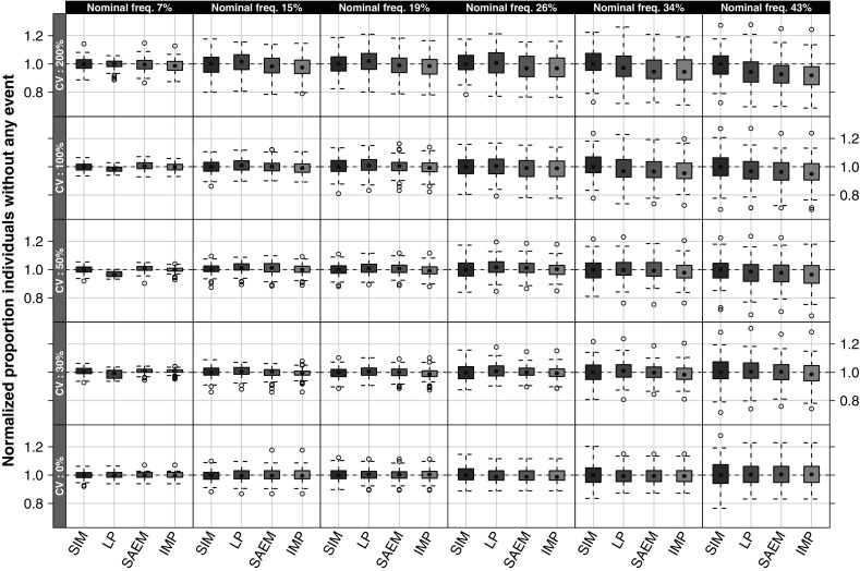
Normalized proportion of individuals without events, stratified on nominal frequency of subjects with events (i.e., when ω ² = 0) and interindividual variability. A value of one indicate that the proportion of events are the same in the average of the original data and in the individual datasets simulated from the true or estimated parameter values, a value higher than one indicates fewer events in the original data than in the re-simulated data. SIM original simulations, LP Laplace, and IMP importance sampling

When comparing the original average number of events per individual with average number of events per individual based on the estimated parameters, all methods were able to capture the original average of number of events per individual when the frequency of at least one event per individual was 15% or higher, shown in Fig. 5. At the lowest investigated frequency, 7%, the Laplace method resulted in a wider distribution of average number of events per individual which is largely affected by the bias in the variance parameter.

Fig. 5.

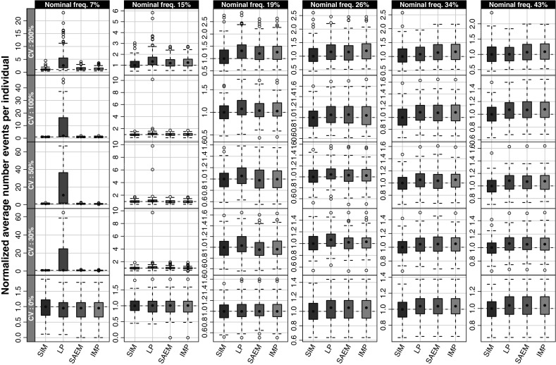
The number of events per individual in the originally simulated data (SIM) and after re-simulation using the parameter estimates from Laplace (LP), SAEM, and importance sampling (IMP) methods normalized to the average number of events per individual under the true parameters. Horizontally the graph is stratified on the variance level and vertically the stratification is made on nominal frequency of subjects with events (i.e., when ω ² = 0)

The runtimes with this model were not an important issue, most runs were finished within seconds. However, the ranking was such that the Laplace method (average runtime of 0.3 s) was faster than the SAEM and importance sampling (average runtimes of 19 and 23 s, respectively). Within each method the trend for Laplace and SAEM was that the runtimes increased with interindividual variability, whereas the opposite behavior was noted for importance sampling. When no interindividual variability was present in the data the SAEM method exhibited on average the longest runtimes with several estimations with runtimes over 100 s.

The stability of the estimations was over all high, the rate of successful minimization (Laplace) or convergence (SAEM and importance sampling) were close to 100% in most scenarios. The SAEM failed to reach convergence in approximately 10% of the estimations when there was no interindividual variability present in the hazard (0 CV%).

DISCUSSION

The Laplace method depends on the empirical Bayes estimates to be a good approximation. For these types of low information content data this is not the case, as have previously been discussed by e.g., Jönsson et al. (5). When the number of events in the study is low there is little information in the data to allow separation between theta and omega. Relatively small model misspecifications can give rise to large deviation in parameter estimates from true values. Main features of the data such as average number of events and fraction of individuals without events are, however, relatively well retained in the model.

At low frequencies of individuals with events within the population (less than 20%), the Laplace method resulted in biased parameter estimates. As has previously been shown with ordered categorical data (5), the bias was particularly evident in the variance parameter which was extremely inflated in many of the estimated datasets. The estimation of the baseline hazard (the fixed-effects parameter) also resulted in biased parameter estimates. The bias in the baseline hazard was negative, indicating an underestimation of the parameter compared to the true values. When comparing outcome measurements, such as average number of events per individual or normalized proportions of individuals without events, these parameter biases were not as apparent (except in the case of very low frequency of individuals with events of 7%). The reason for that is the strong correlation between the estimates of the fixed effect parameter and the variance parameter meaning that an underestimated baseline hazard gives an overestimated variance leading to a net effect on the outcome measurements close to the true data distribution.

The two EM algorithms, SAEM and importance sampling, performed equally well exhibiting no appreciable bias in the baseline hazard. A positive bias in the variance parameter was noted when the interindividual variability was less than 100% and the frequency of individuals with events less than 43%. This is attributable to the fact that in these scenarios there are few individuals who actually experience several events, i.e., there is little support for the variance parameter in these data. Compared to the variance parameter estimates reported by the Laplace method, the SAEM and importance sampling estimates are much closer to the true values.

For all methods, the imprecision in the parameter estimates increases when the information in the data decreases, i.e., when the frequency of individuals with events decreases. When the number of events in the studies is low the relative difference in informativeness between having e.g., eight or ten events in the study becomes large and that is reflected in the imprecision in the fixed-effects parameter estimates. The same reasoning applies to the explanation of the increased imprecision when the interindividual variability (CV%) is decreased, the information about the interindividual variability is then doubled if two individuals compared to one have repeated events whereas if the CV% is high there will be at least a few patients with repeated events in all studies, hence containing more information about the random-effects parameter.

The scenario with 7% frequency of individuals with events and 30% CV was repeated with 1,200 individuals and the overall trends between the methods were the same as with the smaller sample size. However, the RMSE in the fixed effect and the random effect parameter was increased with Laplace and decreased with SAEM and importance sampling, where SAEM was clearly lower. The number of iterations in the importance sampling had to be increased to 1,000 to reach convergence and it is possible that the results can be further improved by changing other settings, like the number of individual samples.

Ueckert et al. (21) have recently demonstrated that the final parameter estimates produced by the SAEM method and the importance sampling methods (implemented in NONMEM 7) can be largely dependent on the initial values of the parameters. Throughout this study, the parameter values used to simulate data were also used as initial values in the estimations, which reduce the parameter bias introduced by bad initial estimates. Moreover, in the investigation by Ueckert and colleagues, the RTTE model was reasonably insensitive to the initial estimates for all parameters, in all three estimation methods—Laplace, SAEM, and importance sampling.

When using EM algorithms there is no formal convergence criterion for of the likelihood, the iterative process continues until a user-defined limit of iterations is reached, preferably when a stable objective function value is reached. The number of iterations needed differs between different methods (i.e., SAEM and importance sampling) and different data sets. If the iteration limit is too low the parameter estimates may be biased due to that the method not having reached the maximum likelihood. On the other hand, if the limit of iterations is very high the estimation may result in unnecessary long runtimes. In the implementation of the EM algorithms in NONMEM, a convergence criteria has been supplied, the convergence criteria can be applied on OFV and fixed-effects parameters or OFV, fixed-effects, and diagonal random-effects parameters or OFV and all parameters, the iterative process will then be aborted when the criteria are fulfilled. To make the comparison between SAEM and importance sampling as fair as possible, the convergence criteria on OFV, fixed-effects, and diagonal random-effects parameters was used in both methods throughout this study.

Although the SAEM and importance sampling are not new methods, the implementation of these in NONMEM 7 offers a great opportunity for the NONMEM oriented modelers to choose the method best suited for the problem at hand. No alternative software needs to be acquired and learned and no additional data management (i.e., new datasets) is needed.

CONCLUSIONS

In terms of bias and precision, SAEM or importance sampling should be the preferred methods when dealing with very low numbers of repeated event data, i.e., rare events. When approximately half of the individuals or more in the study experience events, the performance of the Laplace, SAEM, and importance sampling methods are very similar. The bias and imprecision in the parameter estimates do not severely affect the re-simulation of the actual events of the original design.

Appendix

References

- 1.Harville DA, Mee RW. A mixed-model procedure for analyzing ordered categorical-data. Biometrics. 1984;40(2):393–408. doi: 10.2307/2531393. [DOI] [Google Scholar]
- 2.Stiratelli R, Laird N, Ware JH. Random-effects models for serial observations with binary response. Biometrics. 1984;40(4):961–971. doi: 10.2307/2531147. [DOI] [PubMed] [Google Scholar]
- 3.Cox EH, Veyrat-Follet C, Beal SL, Fuseau E, Kenkare S, Sheiner LB. A population pharmacokinetic-pharmacodynamic analysis of repeated measures time-to-event pharmacodynamic responses: the antiemetic effect of ondansetron. J Pharmacokinet Biopharm. 1999;27(6):625–644. doi: 10.1023/A:1020930626404. [DOI] [PubMed] [Google Scholar]
- 4.Plan EL, Karlsson KE, Karlsson MO. Approaches to simultaneous analysis of frequency and severity of symptoms. Clin Pharmacol Ther. 2010;88(2):255–9. doi: 10.1038/clpt.2010.118. [DOI] [PubMed] [Google Scholar]
- 5.Jonsson S, Kjellsson MC, Karlsson MO. Estimating bias in population parameters for some models for repeated measures ordinal data using NONMEM and NLMIXED. J Pharmacokinet Pharmacodyn. 2004;31(4):299–320. doi: 10.1023/B:JOPA.0000042738.06821.61. [DOI] [PubMed] [Google Scholar]
- 6.Lin X, Breslow NE. N.E. Bias correction in generalized linear mixed models with multiple components of dispersion. J Am Stat Assoc. 1996;91:1007–16. doi: 10.2307/2291720. [DOI] [Google Scholar]
- 7.Rodriguez G, Goldman N. An assessment of estimation procedures for multilevel models with binary responses. J R Stat Soc, Ser A Stat Soc. 1995;158:73–89. doi: 10.2307/2983404. [DOI] [Google Scholar]
- 8.Lavielle MaS, R.M. A new SAEM algorithm for ordered-categorical and count data models: implementation and evaluation. PAGE 18 (2009) Abstr 1526 [wwwpage-meetingorg/?abstract=1526]. 2009.
- 9.Lavielle M. Monolix user's manual. 31. Orsay: Laboratoire de Mathematiques, U. Paris-Sud; 2007. [Google Scholar]
- 10.Bauer RJ, Guzy, S. Monte Carlo parametric expectation maximization method for analyzing population PK/PD data. In: D'Argenio DZ, editor. Advanced methods of PK and PD systems analysis. 2004. p. 135–63.
- 11.Bauer RJ. S-ADAPT/MCPEM user's guide. CA: Berkeley; 2008. [Google Scholar]
- 12.PDx-MCPEM User's Guide. 2006.
- 13.Bauer RJ, Guzy S, Ng C. A survey of population analysis methods and software for complex pharmacokinetic and pharmacodynamic models with examples. AAPS J. 2007;9(1):E60–E83. doi: 10.1208/aapsj0901007. [DOI] [PMC free article] [PubMed] [Google Scholar]
- 14.Dempster AP, Laird NM, Rubin DB. Maximum likelihood from incomplete data via Em algorithm. J R Stat Soc B Methodol. 1977;39(1):1–38. [Google Scholar]
- 15.Beal SL, Sheiner LB, Boeckmann A, Bauer RJ. NONMEM user's guide (1989–2009) Ellicott City: Icon Development Solutions; 2009. [Google Scholar]
- 16.Beal SL, Sheiner LB, Boeckmann A, Bauer RJ. NONMEM User's Guide—Introduction to NONMEM 7. Ellicott City: Icon Development Solutions; 2009. [Google Scholar]
- 17.Beal SL, Sheiner LB. NONMEM user's guide—part VII: conditional estimation methods. Ellicott City: Icon Development Solutions; 2009. [Google Scholar]
- 18.Pinheiro JC, Bates DM, Lindstrom MJ. Model building for nonlinear mixed effects models. American Statistical Association 1994 Proceedings of the Biopharmaceutical Section. 1994: 1–8 522.
- 19.Delyon B, Lavielle V, Moulines E. Convergence of a stochastic approximation version of the EM algorithm. Ann Stat. 1999;27(1):94–128. doi: 10.1214/aos/1018031103. [DOI] [Google Scholar]
- 20.Lindbom L, Ribbing J, Jonsson EN. Perls-speaks-NONMEM (PsN)—a Perl module for NONMEM related programming. Comput Meth Programs Biomed. 2004;75(2):85–94. doi: 10.1016/j.cmpb.2003.11.003. [DOI] [PubMed] [Google Scholar]
- 21.Ueckert S, Johansson ÅM, Plan EL, Hooker AC, Karlsson MO. New estimation methods in NONMEM 7: evaluation of robustness and runtimes. PAGE 19 (2010) Abstr 1920 [wwwpage-meetingorg/?abstract=1920]. 2010. [DOI] [PubMed]