Estimating implant survival in the presence of competing risks

Abstract

In medical research, commonly, one is interested in the time to the occurence of a particular event, such as the revision of an implant, and the analysis of these data is referred to as survival analysis. However, for some patients, the event is not observed and their observations are censored. These censored observations are particular to survival data and require specific methods for estimation. The Kaplan and Meier method is a popular method to estimate the probability of being free of the event over time and it is now widely applied in orthopaedics such as to report implant survival. However, one of the assumptions underlying the Kaplan-Meier estimator implies that patients whose observations are censored have the same risk of occurrence of the event than patients remaining in the study. However, because the revision of an implant cannot occur after a patient dies, and that dead patients have their observations censored in the Kaplan-Meier method, another setting must be considered. In the sequel we will demonstrate the inadequacy of the Kaplan-Meier method to estimate implant survival and detail the cumulative incidence estimator.

Introduction

In medical research, not infrequently, one is interested in the time to the occurence of a particular event, such as the death of a patient, the recurrence of a cancer, or the revision of an implant. Such data are generically referred to as survival data and survival analysis refers to the analysis of these data in the form of delays from a time origin to the occurrence of the event of interest, the end-point. However, for some patients, the event is not observed during the course of the study and their observations, deprived of a survival time, are said to be censored. These censored observations are particular to survival data and require specific methods for estimation.

In 1958, Kaplan and Meier [14] proposed a non parametric method to estimate the survivor function that allows one to determine the estimated survival probabilities from a set of observed data. It is not surprising that this estimator became popular to estimate the occurrence of events other than death, and in 1980 Dobbs [8] was the first to report the implant survival on 400 Stanmore total hip arthroplasties with metal on metal bearings using the Kaplan-Meier method. However, one of the assumptions underlying the Kaplan-Meier estimator implies that patients whose observations are censored, such as those of patients who have not been revised and die during follow-up, have the same risk of occurrence of the event as patients remaining in the study. However, because the revision of an implant cannot occur after a patient dies, another setting must be considered.

The use of the competing risks setting allows one to account for the differences between censoring mechanisms from one observation to another, and the cumulative incidence function gives an appropriate estimate of the cumulative probability of revision of the implant over time in such situations. In the sequel we will show the inadequacy of the Kaplan-Meier method to estimate implant survival and detail the cumulative incidence estimator.

Analysis of survival data with the Kaplan-Meier method

Kaplan-Meier estimate for patient death

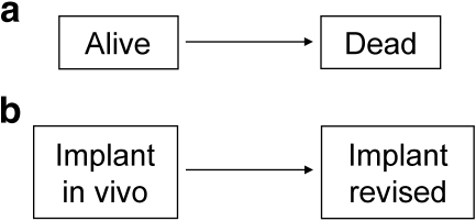
Survival data occurs when one is interested in the time to the occurence of a particular event, for instance death. In that case, one is interested in the transfer from the “alive” state to the “dead” state (Fig. 1a), and the probability that the actual survival time T (which may or may not be observed during study follow-up) of a patient be equal or superior to a time of interest t is called the survivor function: S(t) = Pr(T ≥ t). The objective of survival analysis is to estimate this function and, for instance, be able to predict the probability for a patient of being alive five years after the treatment of a cancer. Understanding the analysis of survival data for patient death is a necessary prerequisite for understanding the analysis of survival data for other events such as implant revision.

Fig. 1.

States and transfers considered in a one transition model, such as the Kaplan-Meier method, for patient (a) and implant (b) survival

There are two reasons why survival data are not amenable to standard statistical methods. The first is that survival times, that is, times from a time origin to the time of occurrence of the event, are not symmetrically distributed. Indeed, survival data usually demonstrate a longer right tail owing to a low number of observations with short survival times. This could be easily dealt with by first transforming the data, for instance, by taking logarithms so as to obtain a more symmetric distribution. However, the main problem encountered when dealing with survival data is that the event of interest is not observed for all patients and the observations of these patients are censored. Censored observations may occur because a patient has been lost to follow-up or because at the end of the study the patient is still alive. Although theoretically the study could be long enough so that every single patient dies during the study time, some patients will still be lost to follow-up and one would still have to deal with these censored observations.

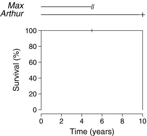
The problem posed for patients with censored observations is that their actual survival time T is unknown and we are unable to analyse the data in a straightforward manner. Figure 2 (top) depicts the follow-up of two patients during a study.

Fig. 2.

Estimation of the survival probability of an event such as death or implant revision with the Kaplan-Meier method

The first patient, Max, is lost to follow-up after five years and the second, Arthur, dies at ten years. The survival time of Arthur is straightforward, it is ten years. However, there is a problem with Max, i.e. we do not know her actual survival time. We could simply consider her observation as missing but doing so we would loose some very important information, that is, Max has survived at least five years. We could also consider that her survival time is five years but then it would mean that she actually died at five years which is not true. The answer to this problem is to consider that Max survived five years and that after five years she survived for some unknown time that we have to account for in some way. Kaplan and Meier [14] proposed that if we consider that the risk of death of patients whose observations are censored is equal to that of the patients remaining in the study, then we can estimate the survival at time t by the cumulative product of the conditional probabilities of surviving each time interval until the chosen time. For instance, Fig. 2 (bottom) shows the Kaplan-Meier estimate of the survivor function for Max and Arthur. Until the fifth year the estimated survival is 100% since no event occurs. At five years, Max is lost to follow-up. From the fifth to the tenth years, no event occurs so the estimated survival is still 100%. At ten years, Arthur only remains in the study and dies but, strangely, the estimate of the survival is not 50% (one event in two patients), it is 0%. The reason for this is that Max, who was lost to follow-up at five years, has been removed from the risk set, namely, the set of patients still under follow-up and at risk of the event, and therefore the force of the following event is increased accordingly (one event in one patient instead of one event in two patients). No estimate is available after ten years since no patient is followed-up beyond that time. Of course this effect is more subtle when more patients are considered, but the principle remains the same, i.e. each time an observation is censored, the force of all following events is increased.

Kaplan-Meier estimate for implant revision

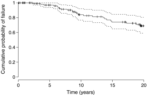
Following the report by Dobbs [8], the Kaplan-Meier estimator has become very popular among orthopaedic surgeons to estimate the probability of implant revision over time. For instance, Hamadouche et al. [13], in a study of 118 alumina-on-alumina bearing total hip arthroplasties in 106 patients operated upon between 1979 and 1980, reported ten-, 15-, and 20-year implant survivals, with revision of the implant for any reason as the endpoint, of 84% (95% confidence interval [CI]: 77–92%), 74% (95% CI: 65–84%), and 69% (95% CI: 59–80%), respectively (Fig. 3). When modeling implant survival, one is interested in the transfer from the “implant in vivo” state to the “implant revised” state (Fig. 1b), and the observations of patients who do not transit from one state to another during study time are censored. This includes patients lost to follow-up, patients still under observation at the end of study, and patients who died during the study time provided they had not been revised before. Indeed, the Kaplan-Meier method does not differentiate between these three reasons for censoring, and whether the patient is lost to follow-up or dies is treated the same way in the estimation of implant survival.

Fig. 3.

Estimation of the survival for implant revision with the Kaplan-Meier estimate (data from Hamadouche et al. [13])

Let us consider implant survival in two patients, Max and Arthur, such as we did before for patient death. Again, Max is lost to follow-up after five years and Arthur undergoes a revision for aseptic loosening at ten years (Fig. 2). The Kaplan-Meier estimate with implant revision for any reason as the event of interest is 100% until the tenth year and drops to 0% at ten years. Again, the reason for the 0% survival at ten years when only 50% of the implants have been revised is that Max has been withdrawn from the risk set at five years and the force of the following event is increased (1 in 1). This is perfectly understandable since we consider that Max’s risk of revision after she is lost to follow-up is that of the patients remaining in the study; since only one patient remains in the study, when he experiences the event, Max does also and the survival drops to 0%. Now let us imagine that Max was not lost to follow-up at five years but died from an unrelated cause. According to the Kaplan-Meier method, Max’s observation is censored in the same way as described above and the ten-year survival for implant revision remains 0%. However, this time it is not acceptable to consider that Max who died at five years presents the same risk of revision as patients remaining in the study, i.e. we know her risk of having a revision after that time is 0 since she is dead and the estimated implant survival at ten years should be 50% (one event in two patients). Unfortunately, the Kaplan-Meier method does not account for this possibility and we have to consider another setting: the competing risk setting.

Analysis of survival data in the presence of competing risks

Definition

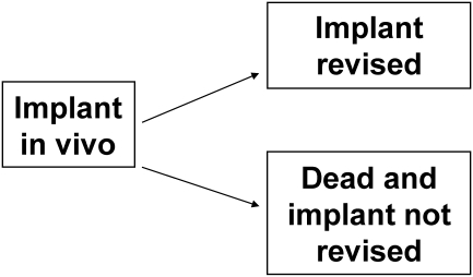
We say that an event is competing with another event when the occurence of the former prevents the occurrence of the latter. The understanding of competing risks dates back to the 18th century when the French mathematician Bernoulli studied the effect of the eradication of smallpox on mortality rates [1]. In a competing event, or similarly competing risk, setting only the occurence of the first of the competing events is of interest because states are absorbing and once a patient falls into a state he or she cannot move to another. Figure 4 presents a competing risk situation where the event of interest is the revision of the implant and where death is competing. In this case, a patient can either experience a revision before dying or die without experiencing a revision. The difference with the Kaplan-Meier estimator is that events other than the one of interest are not made equal. For instance, when estimating implant survival in the Kaplan-Meier setting, whether a patient dies, reaches the end of the study or is lost to follow-up, his or her observation will be censored. On the contrary, in a competing event setting when a patient dies before having his or her hip revised, he or she moves to the “dead and implant not revised” state and cannot move to any other state. Therefore this patient is no longer considered at risk of implant revision. Patients who reach the end of study or are lost to follow-up have their observations censored in the same way as previously described.

Fig. 4.

States and transfers considered in a competing event setting with revision of the implant as the event of interest and death as competing

Cumulative incidence function

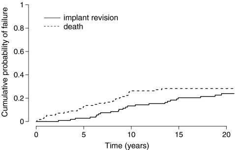
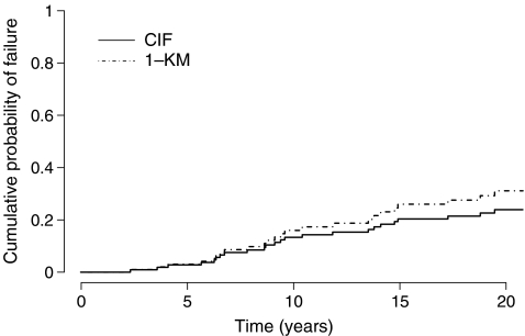
This time we are interested in the probability of failing from cause k before time t : Pr(T ≤ t, D = k). The cumulative incidence function allows us to estimate this probability by summing at any time, over all previous time intervals, the unconditional probabilities of failing from cause k at t _j [15]. This corresponds to the cumulative sums of the event-free survival (i.e. the probability of having none of the competing events by time t₋₁) multiplied by the hazard (i.e. the number of events of interest divided by the number of patients at risk at time t ). Figure 5 shows the cumulative probability with implant revision for any reason as the event of interest and death as a competing event of the patients in the study by Hamadouche et al. [13]. The estimated ten-, 15- and 20-year cumulative probabilities for implant revision are 14% (95% CI: 7%–22%), 23% (95% CI: 14%–32%), and 27% (95% CI: 17%–36%), respectively. It can be seen that, instead of plotting the probability of being free of the event by time t as with the Kaplan-Meier estimate, it is the probability of having the event that is plotted over time. Also, in a competing event, setting it is usual to plot the estimate of the competing events and assess the competition between these events. It must be emphasised that estimating death as a competing event is not the same as death as the only event. In the former case, one estimates the cumulative probability of dying before having a revision and in the latter one estimates the cumulative probability of dying regardless of other events. Figure 6 shows a comparison of the cumulative probability of implant revision estimated with the Kaplan-Meier method (here we plot 1-Kaplan-Meier for comparative purposes) and with the cumulative incidence function. It can be seen that with time, the Kaplan-Meier method overestimates the probability of having the event. The reason is that as time progresses more and more observations are wrongly censored, and each time, the force of the following events is increased. Consequently, the bias in the Kaplan-Meier method inflates. At 20 years, the estimated risk of implant revision is 31% with the Kaplan-Meier method and 27% with the cumulative incidence function. The more patients experience the competing event and the earlier in follow-up, the more this difference will show. In a previous series of 91 tumour knee megaprostheses [2], where patients present a high risk of death during follow-up due to their bone cancer, we reported a 67% risk of revision at 15 years with the Kaplan-Meier method compared to a 47% risk of revision with the cumulative incidence function; in this case the Kaplan-Meier method overestimated the risk of revision by 43% at 15 years [3]. Similarly, when reporting implant survival in young patients, one would expect the bias in using the Kaplan-Meier analysis as being important since many patients are expected to die during follow-up [9, 17].

Fig. 5.

Estimation of the cumulative probability of implant revision with the cumulative incidence function

Fig. 6.

Comparison of the estimation of the cumulative probability of implant revision with the cumulative incidence function and 1-Kaplan-Meier (data from Hamadouche et al. [13])

Conclusion

The use of competing risks in the medical literature is not recent but the attention of orthopaedic surgeons to this method is more recent [3–6, 10, 12]. The Kaplan-Meier method is entirely valid when one is modelling patient survival since it almost never occurs that an event will be competing with death. However, when modelling implant survival using the Kaplan-Meier method, the assumption is made that either patients who die are still at risk of having a revision or that patients do not die. In either case this assumption is not tenable and an alternative method is necessary. The competing event setting adequately accounts for the differences in risk between patients who die and those who are lost to follow-up or have reached the end of the study without experiencing a revision. The cumulative incidence function allows estimation of the probability of implant revision and gives insights on the competition between events.

Two issues which are a little more complex may be of interest. First, when one is interested in estimating the effect of a covariate on survival, the model of choice is that proposed by Cox [7] and known as the Cox proportional hazard regression model. This model remains valid in the presence of competition and it models the effect of a covariate on the cause-specific hazards. However, the effect of covariates on cumulative incidence curves are no longer easily interpretable. A model to regress directly on the cumulative incidence curves has been developed recently [11]. Second, in the competing risk setting presented here, we consider one initial state and several mutually exclusive absorbing states. However, this does not account for reality. Indeed a patient will die after a revision and also a patient who undergoes a revision will have another prosthesis implanted that may possibly require another revision. In fact, competing risks are only a particular case of more complex multi-state models where patients are allowed to transfer almost (death remains absorbing) freely between all states [16].

References

- 1.Bernoulli D (1760) Essai d’une nouvelle analyse de la mortalité causée par la petite vérole, et des avantages de l’inoculation pour la prévenir. Mémoires de l’académie Royale des Sciences Paris, pp 1–45
- 2.Biau D, Faure F, Katsahian S, Jeanrot C, Tomeno B, Anract P. Survival of total knee replacement with a megaprosthesis after bone tumor resection. J Bone Joint Surg Am. 2006;88:1285–1293. doi: 10.2106/JBJS.E.00553. [DOI] [PubMed] [Google Scholar]
- 3.Biau DJ, Latouche A, Porcher R. Competing events influence estimated survival probability: when is Kaplan-Meier analysis appropriate? Clin Orthop Relat Res. 2007;462:229–233. doi: 10.1097/BLO.0b013e3180986753. [DOI] [PubMed] [Google Scholar]
- 4.Biau DJ, Davis A, Vastel L, Tomeno B, Anract P. Function, disability, and health-related quality of life after allograft-prosthesis composite reconstructions of the proximal femur. J Surg Oncol. 2008;97:210–215. doi: 10.1002/jso.20936. [DOI] [PubMed] [Google Scholar]
- 5.Biau DJ, Larousserie F, Thévenin F, Piperno-Neumann S, Anract P. Results of 32 allograft-prosthesis composite reconstructions of the proximal femur. Clin Orthop Relat Res. 2009;468:834–845. doi: 10.1007/s11999-009-1132-z. [DOI] [PMC free article] [PubMed] [Google Scholar]
- 6.Biau DJ, Thévenin F, Dumaine V, Babinet A, Tomeno B, Anract P. Ipsilateral femoral autograft reconstruction after resection of a pelvic tumor. J Bone Joint Surg Am. 2009;91:142–151. doi: 10.2106/JBJS.G.01061. [DOI] [PubMed] [Google Scholar]
- 7.Cox RD. Regression models and life tables (with discussion) J Roy Stat Soc B. 1972;74:187–220. [Google Scholar]
- 8.Dobbs HS. Survivorship of total hip replacements. J Bone Joint Surg Br. 1980;62:168–173. doi: 10.1302/0301-620X.62B2.7364829. [DOI] [PubMed] [Google Scholar]
- 9.Falez F, Favetti F, Casella F, Panegrossi G. Hip resurfacing: why does it fail? Early results and critical analysis of our first 60 cases. Int Orthop. 2008;32:209–216. doi: 10.1007/s00264-006-0313-6. [DOI] [PMC free article] [PubMed] [Google Scholar]
- 10.Fennema P, Lubsen J. Survival analysis in total joint replacement. An alternative method of accounting for the presence of competing risk. J Bone Joint Surg Br. 2010;92:701–706. doi: 10.1302/0301-620X.92B5.23470. [DOI] [PubMed] [Google Scholar]
- 11.Fine JP, Gray RJ. A proportional hazard model for the subdistribution of a competing risk. J Am Stat Assoc. 1999;94:496–509. doi: 10.2307/2670170. [DOI] [Google Scholar]
- 12.Fuchs B, Hoekzema N, Larson DR, Inwards CY, Sim FH. Osteosarcoma of the pelvis outcome analysis of surgical treatment. Clin Orthop Relat Res. 2009;467:510–518. doi: 10.1007/s11999-008-0495-x. [DOI] [PMC free article] [PubMed] [Google Scholar]
- 13.Hamadouche M, Boutin P, Daussange J, Bolander ME, Sedel L. Alumina on alumina total hip arthroplasty. A minimal 18.5 -year follow-up study. J Bone Joint Surg Am. 2002;84:69–77. [PubMed] [Google Scholar]
- 14.Kaplan EL, Meier P. Non parametric estimation from incomplete observations. J Am Stat Assoc. 1958;53:448–457. doi: 10.2307/2281868. [DOI] [Google Scholar]
- 15.Prentice RL, Kalbfleisch JD, Peterson AVJ, Flournoy N, Farewell VT, Breslow NE. The analysis of failure times in the presence of competing risks. Biometrics. 1978;34:541–554. doi: 10.2307/2530374. [DOI] [PubMed] [Google Scholar]
- 16.Putter H, Fiocco M, Geskus RB. Tutorial in biostatistics: Competing risks and multi-state models. Stat Med. 2007;26:2389–2430. doi: 10.1002/sim.2712. [DOI] [PubMed] [Google Scholar]
- 17.Wangen H, Lereim P, Holm I, Gunderson R, Reikeras O. Hip arthroplasty in patients younger than 30 years: excellent ten to 16-year follow-up results with a HA-coated stem. Int Orthop. 2008;32:203–208. doi: 10.1007/s00264-006-0309-2. [DOI] [PMC free article] [PubMed] [Google Scholar]