CytoSolve: A Scalable Computational Method for Dynamic Integration of Multiple Molecular Pathway Models

Abstract

A grand challenge of computational systems biology is to create a molecular pathway model of the whole cell. Current approaches involve merging smaller molecular pathway models’ source codes to create a large monolithic model (computer program) that runs on a single computer. Such a larger model is difficult, if not impossible, to maintain given ongoing updates to the source codes of the smaller models. This paper describes a new system called CytoSolve that dynamically integrates computations of smaller models that can run in parallel across different machines without the need to merge the source codes of the individual models. This approach is demonstrated on the classic Epidermal Growth Factor Receptor (EGFR) model of Kholodenko. The EGFR model is split into four smaller models and each smaller model is distributed on a different machine. Results from four smaller models are dynamically integrated to generate identical results to the monolithic EGFR model running on a single machine. The overhead for parallel and dynamic computation is approximately twice that of a monolithic model running on a single machine. The CytoSolve approach provides a scalable method since smaller models may reside on any computer worldwide, where the source code of each model can be independently maintained and updated.

Introduction

A grand challenge of computational systems biology is to model the whole cell. Biologists use experiments, not first principles or “laws” (ab initio) as in physics, to derive molecular pathways, as shown on the left in Fig. 1, which are the diagrammatic representations of molecular interactions.16 Computational systems biologists translate these molecular pathways into molecular pathway models, as shown on the right in Fig. 1, which are the quantification of molecular interactions. They also work to build large-scale models of cellular function by integrating the biomolecular kinetics across multiple models at the molecular mechanistic level.1,10,13,15,22,26

Figure 1.

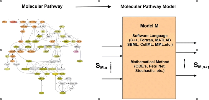
A molecular pathway, represented diagrammatically on the left, can be converted to a molecular pathway model, M, on the right, which receives inputs, S _M,n and evaluates outputs, S _M,n+1 using various mathematical approaches (e.g. ODE’s). The model can be encoded using various programming languages

A molecular pathway model M can be thought of as “black box” which describes the biomolecular kinetics of a set of molecular species, S _M. The input to the black box are the concentrations of species at time t = n, denoted as S _M,n,. The internals of the black box contain computer source codes that evaluate the input using mathematical methods to yield an output. The output of the black box are the concentrations of species at time t = n + 1, denoted as S _M,n+1.

The current methods for integrating models attempt to use direct computation to solve the problem, i.e. developing a program from scratch for each set of coupled reactions, or a monolithic approach, which takes individual component models in a single supported computer source code format such as Systems Biology Markup Language (SBML)11 and manually integrates them to create one monolithic software program. A variation on this second approach is to use semi-automation tools that help to automatically read and integrate source codes together to create one monolithic software program.24 The most common architectures such as Cell Designer,16 COPASI21 or E-CELL,26 use the monolithic approach.

The monolithic approach presents significant hurdles in scaling to large numbers of models. All models have to reside in the same geographical location, and the person integrating the models must be intimately acquainted with all the multiple pathways to be merged. Maintenance of the larger monolithic model emerges as a critical issue since new biological experiments may yield results that require changes to individual molecular pathways and their models’ source codes. If each model is in different source code format, conversion to a single format is required.

This paper describes CytoSolve, a computational environment for integrating multiple independent pathways dynamically in parallel to address the shortcomings of monolithic methods.

Characteristics of a Dynamic Methodology

A method that dynamically integrates the computations of the smaller molecular pathway models may obviate the need to: (1) merge source codes and (2) centrally maintain and update the source codes of each model. In fields such as ecology and earth sciences, platforms such DANUBIA3 have shown the value of integrating distributed models in parallel without the need to merge source codes. There are a number of important characteristics that such a dynamic method should exhibit.

First, it should be scalable. Scalability means the effort to integrate a new model is comparable to the effort to integrate the first model. Scalability has little to do with complexity. Two models with numerous equations, for example, can integrate easily if they are in the same programming language, have similar time scales, belong to the same knowledge domain and were developed on the same hardware and operating systems. Second, the method should be able to connect multiple knowledge domains in an opaque manner; such opacity will treat each model as a “black box” shielding the integrator from internal details. The integrator needs only know the inputs and outputs of each model. This will allow for integration of emerging compartmental models.

Third, the method should provide support for both public and proprietary models. Public models have accessible source codes. Proprietary models have inaccessible source codes. A pharmaceutical company, for example, with proprietary models may seek to integrate with public models, and researchers in an academic environment, alternatively, may seek to integrate their public models with proprietary models. Fourth, it should be extensible to provide support for heterogeneous source code formats including support for long standing formats such as MML generated by JSIM,21 and more recent standards such as SBML and CellML.12 Other important models have been published using programming languages such as MATLAB, Java or C. A computational architecture that supports dynamic integration will not require conversion to one standard format. Keeping a model resident on its native format will reduce time in source code rewriting and testing. An analogy is having a single program to display a collection of digital pictures stored in various graphical formats.

Last, the architecture should support localized integration. This means that users at all locations can initiate integration from their own local environment. Consider the scenario of the author of a Model A, who wishes to quickly test or integrate with an ensemble of three other models: Model B, C and D which are distributed across different machines. The author of Model A should not have to download the other three models to his/her local computer to perform the integration.

Ease of integrating an ensemble of disparate and distributed molecular pathway models, each owned by different authors is therefore critical to building large-scale models such as the whole cell. In his seminal work, Brooks5 demonstrated that as the number of different authors (or models) increases, the effort to perform such integration increases geometrically with the number of personnel communications required to simply coordinate the software development among the different authors. CytoSolve provides a new methodology to integrate models without requiring personnel interaction with the authors since each model need not be manually loaded, understood and interconnected into a single monolithic program.

Architecture

CytoSolve’s parallel and distributed architecture addresses the various scalability problems of integrating multiple models. In this architecture, the whole cell, using the theoretical framework and conditions prescribed in Appendix A, can be viewed as a network of D molecular pathways as shown in Fig. 2a or modelled as an interconnected ensemble of D molecular pathway models, shown in Fig. 2b. CytoSolve as shown in Fig. 2c uses a dynamic messaging approach to exchange data via message passing across the ensemble of models, {M _i} (for i = 1 to D) to evaluate the integrated solution.

Figure 2.

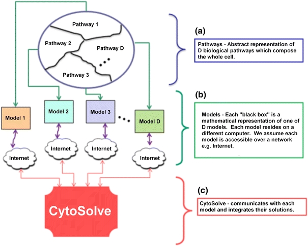
Abstraction of cell being represented as an integration of D molecular pathway models. A large pathway is partitioned to smaller pathways, which are represented as mathematical models that are integrated using the CytoSolve system

CytoSolve computes the integrated solution using the n-tier layered architecture shown in Fig. 3. This architecture consists of the following layers: Presentation, Controller, Communications, Models and Database.

Figure 3.

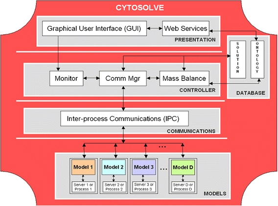
The architecture design underlying the CytoSolve method employs a dynamic messaging approach to manage and integrate communications across a distributed ensemble of D models based on instructions by the GUI at the Presentation layer. The Controller layer integrates the solution among the models using three components: Monitor, Comm Mgr and Mass Balance. The Communication layer provides infrastructure to communicate input and output values across models running as separate processes on a single server or separately on individual servers. The Data Base layer provides storage for the Solution to hold the results of the integrated and individual model solutions along with Ontology for registering and describing each model’s characteristics and annotations made by the user. The Models layer denotes the ensemble of models, which may be remote or local

The Presentation layer includes a Graphical User Interface (GUI) and Web Services. The user interacts with the GUI to specify one or more molecular pathway models to be integrated. A set of molecular pathway models may have common species and/or duplicate reaction pathways. For the former case, e.g. two models may refer to species Calcium but one may have refer it as “Ca++” and another as “Cal”, a Web Service is provided, which parses the models and detects potential naming conflicts and allows the user through the GUI to confirm or reject identical species. The Web Services also provides the user a mechanism to identify common reaction pathways to enable alignment across models. All user-defined changes or such annotations to the models to resolve species differences and reaction duplications are stored and updated within the Ontology of the Database, for later use by the Controller, during model integration. Once the user has specified models and resolved conflicts, the Controller via the Monitor, is invoked for executing model integration.

The Controller coordinates individual computations and couples models to derive the integrated solution. The Controller includes libraries that support direct model-to-model messaging as well as model-to-controller messaging. CytoSolve’s Controller has three components: the Monitor, the Communications Manager (Comm Mgr) and the Mass Balance. The Monitor serves to track the progress of each model’s computation. The Monitor knows, for a particular time step, which models have completed and which models have not completed their calculation. The Comm Mgr or Communications Manager coordinates the communication across all models. The Comm Mgr initiates a model to compute a time step of calculation and also can instruct a model to wait or hold on computing the next time step. The Mass Balance integrates, for each time step, the calculations across an ensemble of models by ensuring mass conservation of species, to derive the integrated solution.

The Communications layer contains the Inter-process Communications (IPC) infrastructure. The IPC allows communication of user parameters (e.g. which models to run) and results between the Controller and the Models. IPC allows the Controller to perform dynamic messaging using two important operations. First, the Controller may message a model with input values of species concentrations at time step n, S _M,n and request the model to execute one time step of calculation. Second, a model, following execution of one time step of calculation, can message the Controller to send the output values of species concentrations at time step n + 1, S _M,n+1. These operations enable the Controller to manage and steer the individual computations across multiple models in parallel.

The Data Base layer consists of storage of the Solution and the Ontology. The Solution (as detailed in Appendix B) holds memory resident data to track species concentrations across all models for each time step. The Ontology manages nomenclature and the annotations of species identification and duplicate reaction pathways, across models to ensure consistency during the Controller’s computation of the integrated solution (see Appendix C). The Ontology can be evolved to support more complex descriptions.

The Models layer denotes the set of models to be integrated. These models may each reside on different servers, remote to the GUI. Or, the models may reside on a single server, possibly the same server as the GUI, but may run as individual processes. CytoSolve treats each model as a module whose model code can be as simple or as complex as possible. However, what is important is the format of the inputs and outputs to and from the model, respectively. Appendix D provides a diagrammatic representation of a model, its input and outputs and how these inputs and outputs are linked with the temporal inputs and outputs of other models to evaluate a solution.

Implementation

CytoSolve is implemented using open source software to reduce expense and to ensure that future work can be pursued with minimal reliance on proprietary tools. Figure 4 illustrate the components used at various layers of the CytoSolve architecture. At the Presentation layer, the web-based GUI currently implemented using the Java language running on Apache Tomcat,7 can also easily be implemented in PHP or ASP, for example. The GUI allows a user multiple ways to run and couple model(s): (1) Execute a model(s) local to the GUI as multiple processes; (2) Execute a models remote to the GUI; (3) Execute in parallel a model locally and multiple models on remote servers; and (4) Execute all models on remote servers and couple their results. The Web Services are written in J2EE.

Figure 4.

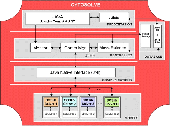
The implementation of CytoSolve is done using open source tools as indicated at each layer

At the Controller layer, the three components, Monitor, Comm Mgr and Mass Balance, are programmed using J2EE. The Controller is executed on a Pentium 4 CPU 3.00 GHz Dell Workstation with 2 GB of RAM running Windows XP with Service Pack 2. Each component can be multi-threaded and communicates using message passing. At the Data Base layer, Virtual Memory is allocated for the Solution storage (as detailed in Appendix B) and a Java DB and ASCII files are used for the Ontology (as described in Appendix C).

At the Communications layer, IPC were originally implemented using the Simple Object Access Protocol (SOAP),23 but for performance reasons have been rewritten using the Java Native Interface (JNI lib).19 This XML-based messaging format established a transmission framework for IPC communication via HTTP. Both SOAP and JNI are vendor-neutral technologies that provide attractive alternatives earlier protocols, such as CORBA or DCOM. The Web Services Description Language (WSDL)6 supplied a language for describing the interface of the web services.

The Models used in the implementation are written in SBML and were acquired from the BioModels Database17 which provides access to published, peer-reviewed, quantitative models of biochemical and cellular systems delivered in SBML and CellML formats.

The CytoSolve architecture uses an interpreter to enter reaction and specie data relative to the pathway. In the current production version, we provide an input filter only for models coded in SBML. Other input filters for models stored in other formats can be incorporated within the architecture, provided the input filter for that format is developed and tested. In our earlier internal development efforts, we have produced prototype input filters for model formats written in MATLAB and Java. Our development roadmap, for future production versions looks to release these and other input filters to support CellML and MML. Such development may occur by our research team or through collaboration with the developers of those two formats.

Fundamentally, CytoSolve treats each individual pathway as a “black box” to which input concentrations are sent and from which time-evolved outputs are received. In principle, CytoSolve’s architecture is not dependent on the internal computational methods e.g. ODE, Petri Net, Stochastic, etc., for evaluating the models dynamics, nor the source code formats they are written. As aforementioned, MATLAB representations in parallel with SBML ODE solvers have been tested in earlier versions. The critical issue for integrating the black boxes across different computational methods is the pre-computational alignment of the individual pathways. This requires that the species and the equations be precisely defined such that common species and common pathways among models are identified. We are developing automated methods to do this for pathways expressed in SBML that we believe can likely be generalized to CellML and MML. We do not have standard packages to do this with models written in C and MATLAB, however, for example. For those cases, the alignment between the different pathways would have to be done by hand.

The web-based GUI, recently ported from a non-GUI environment, currently runs on a server through a web connection to http://www.cytosolve.com. The browser is cross-platform a design that can be run on workstations, laptops and even mobile devices such as the iPhone. The servers which the Models run on is a Pentium 4 CPU 3.00 GHz Dell Workstation with 2 GB of RAM running Windows XP with Service Pack 2, or a Mac Pro Server with two Intel quad-core processors with 4 GB of RAM running OSX10.6 (Snow Leopard).

The SBML ODE Solver (SOS) library (SOSlib)20 is used to enable symbolic and numerical analysis of chemical reaction networks. SOSlib takes as input a file encoded in the SBML and computes time history of species concentrations for specified initial conditions and time steps. In this implementation, the SOSlib was modified, using the C programming language, to enable single time-step evaluation. Other solvers supporting CellML, MML,4 and other pathway description dialects can be used interchangeably with SOSlib. Even MATLAB programs have been used. After the setting of the parameters, the model(s) are executed and the results are displayed and stored. An Appendix E has been added which provides the main steps for using the CytoSolve system. As the web-based environment is new and developing, documentation, on-line help, tutorials and video demonstrations are forthcoming and being updated to provide more detailed instructions.

Computational Methodology

CytoSolve dynamically integrates the computations of each model M to derive the species concentration of the integrated model O (derived in Appendix A), denoted as S _O (defined in Appendix B). The flow chart of the computational methodology is illustrated in Fig. 5.

Figure 5.

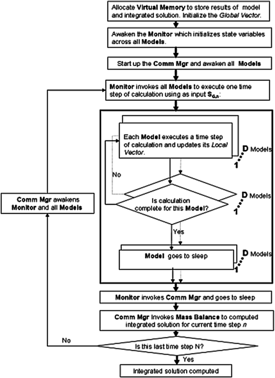
The flow chart of CytoSolve’s computational methodology

The Controller performs initialization of the system by allocating memory storage for the computed species concentrations of each model and the integrated model in Local Vectors, and Global Vector, respectively, as detailed in Appendix B. During this initialization, the initial species concentrations, S _O,0, are set in the Global Vector. In addition, CytoSolve during this initialization performs various types of pre-checks on models prior to integration.

One pre-check is to ensure coordination of physical dimensions e.g. conversion of species concentrations to uniform units, for example, molecules/cell or nM units. The other pre-check is to ensure coordination of common species, e.g. conversion of species names referring to the same species to a uniform name, for example, “Ca++” or “Calcium”. Finally, one other pre-check is to ensure coordination of common pathways, e.g. conversion of reactions referring to the same reaction to a consistent and common one. For the coordination of physical dimensions, CytoSolve currently performs unit checking and unit conversion on all input parameters. This is done both at the species level and at the equation level. For the latter two pre-checks, coordination of species names and pathways, CytoSolve uses a graph-theoretic approach, based on reaction-component (species) reachability to identify duplicate graph (reaction) pathways. A combination of Uniprot ID’s and sub-string matches are used to identify common species and duplications to align the graphs. During pre-checking, the user is alerted on any inconsistencies across species naming. In that event, the user can confirm or reject CytoSolve’s identification of common species. The user’s changes are annotated and both the Uniprot ID’s and species names in the model are updated.

Monitor, which monitors the progress of each model’s computation, during its initialization, accesses the initial conditions, S _O,0, from the Global Vector, and sets these as the initial conditions for each model’s species concentration, S _M,0. Control is then passed to the Comm Mgr which awakens all the models to start up and become ready to process a time step of calculation, and then invokes the Monitor.

The Monitor proceeds to invoke all models in parallel to execute a time step of calculation using S _O,n, the species concentration values of the integrated model O at time step n, as the input to all models. Each model executes and computes one time step of calculation on its own Remote Server. Monitor tracks the progress of each model’s completion. Once a model completes its computation, the output is stored in its Local Vector within the Virtual Memory, and the model then goes to sleep to optimize use of the Remote Server’s CPU usage. By sleep, we mean that the model goes dormant until invoked again by the Comm Mgr to process another time step of calculation. Once all models have completed their processing for a time step, the Monitor passes control back to the Comm Mgr, and the Monitor itself goes to sleep.

Once all models have completed a time step of calculation, the Comm Mgr invokes Mass Balance to dynamically couple the computations at time step n of each Model to evaluate the integrated model O solution S _O. Using the derivation in Appendix B, the Mass Balance component of the architecture, using Eq. (1), after each time step, n, calculates local species concentration changes of each model denoted as;

1

where S _M,n is input to model M containing species concentration values at time step n; S _M,n+1 is output from model M containing species concentration values at time step n + 1; i references a model with i = 1 to D, with D being the total number of models; j references a molecular species with j = 1 to C, with C being the total number of unique molecular species across the union of all models M. Any one model may only utilize a subset of those C species; and, n references time step with n = 0 to N − 1, where N being total number of time steps; and,

Mass Balance adds these local changes to the integrated model’s species concentration values for the current time step, S _O,n, to compute the species concentration, S _O,n+1 at the next time step, n + 1, as denoted in Eq. (2).

2

where S _O,n is the time-evolved solution of the integrated model O at time step n; S _O,n+1 is the time-evolved solution of the integrated model O at time step n + 1.

NOTE: The Mass Balance component uses the Ontology (as described in Appendix C), to ensure that the species identities are correct. For example, if two different nomenclatures (e.g. Ca++ and CALCIUM) exist for the same species, and the species are treated as different, then one species may get depleted while the other floats at near its original value, which is not going to give the correct result. The Ontology is therefore critical in ensuring the species identification across models is correct.

If the last time step has been computed, the Controller stops, performs a variety of cleanup functions to release resources, memory, etc., and returns control back to the GUI; otherwise, the Comm Mgr cycles again for the next time step. All models, even those with different time scales, as of now are invoked with a homogeneous time step. This will be area for future research as noted in the sub-section “Adaptive Time Stepping of the Controller” in the “Discussion and Conclusions” section.

Currently CytoSolve is only concerned with the concentrations of species changes at each time step, and has limited its input output stream to these values; however, the architecture supports transfer of other attributes, which could be invoked, tracked and coordinated by the Controller.

Validation of Cytosolve

CytoSolve is validated by comparing the solution it produces with the one generated by Cell Designer, a popular tool for building molecular pathway models in a monolithic manner. As a control, the Epidermal Growth Factor Receptor (EGFR) model published by Kholodenko14 is selected for this comparison. Snoep25 have authored the model into the SBML language. The entire EGFR model, as shown in Fig. 6, is loaded into Cell Designer and executed on a single computer.

Figure 6.

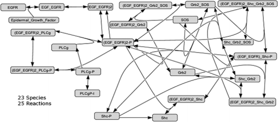
Complete EGFR model of Kholodenko implemented in Cell Designer on a single computer

The same entire EGFR model, to test CytoSolve, is split into four models and distributed on four different computers as shown in Fig. 7.

Figure 7.

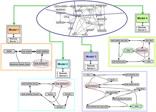
Complete EGFR model of Kholodenko split on four remote servers for CytoSolve solving

Note, in Fig. 7, that species (EGF_EGFR)2-P, encircled in red, is shared by all four models; however the species SOS, encircled in green, is shared only between two models. CytoSolve and Cell Designer are run for a total of 10 s in simulation time.

Results

CytoSolve and Cell Designer produce near exact results as shown for two example species in Fig. 8.

Figure 8.

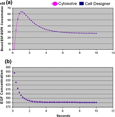
Comparison of results from CytoSolve and Cell Designer for two species. (a) Compares values of the EGF-EGFR species. (b) Compares values of EGF concentration

The results in Table 1, column 1, provide the percent (%) in difference of the solutions calculated using CytoSolve and Cell Designer. The Solution Difference is calculated as an average of the percent (%) difference for each species, over five test runs. None of the solutions diverged. The small differences are a result of the selection of the time step, which presents some important and subtle issues. The selection of the time step is discussed in the sub-section entitled “Optimization of Time Step Selection” in the “Discussion and Conclusions”.

Table 1.

Comparison of cytosolve and cell designer

Solution Difference (%)	CytoSolve compute time (ms)	Cell Designer compute time (ms)
0.026	5932	3217

Column 1 compares the % difference in solutions. Column 2 and column 3 compare the compute time differences

Column 2 and Column 3 in Table 1 provide the compute times for using CytoSolve and Cell Designer, respectively. CytoSolve’s compute time is roughly twice that of Cell Designer. The additional compute time is primarily due to network latency required for CytoSolve’s Controller to contact and receive information back from each model running on different Remote Servers. Cell Designer has no network latency since each model runs on a single computer.

Discussion and Conclusions

This paper has introduced CytoSolve, a new computational environment for integrating biomolecular pathway models. The initial results from the EGFR example has demonstrated that CytoSolve can serve as an alternative to the monolithic approaches, such as Cell Designer. Most important is CytoSolve’s core feature for integrating multiple pathway models, which can be distributed across multiple computing systems and solved in parallel, obviating the need to merge models into one system, running on a single computer. In the EGFR example, this means that if changes are made to Model 1, in Fig. 7, then CytoSolve simply has to be executed to evaluate a new solution; however, Cell Designer will require that changes to be manually merged back into the whole model and then executed. So in practicality, if each Model (1, 2, 3 and 4) is each owned by different authors, who make changes, then constant maintenance will be needed using Cell Designer to ensure the model is up to date.

The purpose of CytoSolve is to offer a platform for building large-scale models by integrating smaller models. Clearly, modeling the whole cell from hundreds of sub-models, each of which is owned by various authors (each making changes to their models) using the monolithic approach is not scalable. CytoSolve’s dynamic messaging approach offers a scalable alternative since the environment is opaque (treats each model as a black box) support for both public and proprietary models is extensible to support heterogeneous source code formats, and finally supports localized integration, a user can initiate integration from their own local environment.

From CytoSolve’s viewpoint a sub-model or module is a “black box”. We are agnostic to the meaning of that module and its biological context, and CytoSolve will simply integrate any set of modules. The user can of course intervene and decide which species are duplicates and provide context through the user interface. CytoSolve’s requirement, therefore, in this aspect, is minimal: each sub-model or module must accept as input a vector of species concentrations at a particular time step, and provide an output vector of species concentrations at the next time step.

Two other systems, CellAK and Cellulat, also offer an alternative to the monolithic approach.9,28 However, both of them use a static messaging approach. In the static messaging approach, the models remain independent programs and do not affect each other as they are executing. Any one model accepts as input a dataset and executes to completion to generate an output dataset. That output dataset is then given to another model, which that model uses it as input and also executes through to completion. This process can then be continued with other models, and they can be executed concurrently if there are no dependencies between their datasets.

CellAK and Cellulat treat each biological pathway model as a single entity (or agent) obeying its own pre-defined rules and reacting to its environment and neighboring agents accordingly. These two approaches offers many positive ways for integrating biomolecular pathway models; however, a non-specialist has a very high learning curve in preparing a set of biological pathway models for use with this approach because the integrator has to understand deeply the biology and architecture behind them. Furthermore these tools do not use ordinary differential equations to determine the time evolution of cellular behavior, since differential equations find it difficult to model directed or local diffusion processes and sub-cellular compartmentalization and they lack the ability to deal with non-equilibrium solutions. Most common biological modeling systems use traditional ODEs to simulate the models. Finally these two approaches are not designed to perform simulations on a distributed computational environment, which CytoSolve offers.

The implementation of CytoSolve to enable distributed and parallel computations across an ensemble of models also presents many new and unique challenges. Such challenges include the need to advance and optimise elements of the architecture, which particularly becomes relevant in a software implementation, which is a dynamic work in progress. These challenges have become important areas for our ongoing research, some of which are noteworthy to discuss in this manuscript.

Optimization of Time Step Selection

CytoSolve’s Controller, for example, ensures mass conversation of all species in the integrated molecular network. To ensure thermodynamic feasibility, however, the detailed balance constraint, which demands that at thermodynamic equilibrium all fluxes vanish must be imposed during computational integration by the Controller.8 This is a subtle but important issue that CytoSolve is aware of, which becomes apparent during the Controller’s evaluation of a common species concentration, across a set of models. To discuss by example, consider the case of two models, both with large rate constants, which share a common species, that are being communicated through the Controller. In this case, detailed balance demands that the associated species concentrations balance each other off. However, if the two opposing reactions do not communicate, the computational problems become far more difficult. Whereas, if the two competing rates net to zero the solution is stable and expressible as a simple ratio of concentrations. Segmenting the two competing rates into two separate independent pathways requires high accuracy calculations and a very small time step for the finite difference calculation to achieve a stable equilibrium meeting the requirements of detailed balance, one that will always be slightly displaced from the “true” equilibrium solution. We recognize that the displacement error is probably infinitesimal compared to the probable error in the reaction rates used in the calculation, but it is nonetheless a finite calculable error. The accurate and optimal selection of the time step during integration must be small to keep the error of species concentration, at each time step to an acceptable level. We are aware of this problem and are currently examining efficient ways to select time steps, by sharing information across pathways.

Spatial Scale Variation

At the present time, CytoSolve supports only computational models that represent one single pool of material or several distinct pools connected with specific transport relations. We have not considered changes in concentrations on a continuous spatial scale. We believe that the architecture, based on its modular approach and support for multiple compartments, can support varying spatial scales. However, more testing will have to be performed to understand the computation times required to fully support such spatial variations. The description language FieldML is available to support this process.

Adaptive Time Stepping of the Controller

All models are currently computed using a single adaptive time step, which is taken to be the fastest time step among the ensemble of models. This is not optimal, as some component models may be varying more slowly than others. Additional effort is required to implement intelligent adaptive time stepping at the Controller level to observe the time scales of different models and invoke them only when necessary. Such an effort will result in improved computation time performance.

Stiffness of ODE Systems

Stiffness is a common problem of ODE systems where integration of molecular pathway models may involve processes at different time scales. While adaptive time steps at the Controller level (during integration) will help towards addressing this problem, control of the ODE solver for simulation of sub-models will also be necessary. The current method within CytoSolve is to choose the time constant sufficiently small that additional decreases in the time step do not lead to different results. We are currently pursuing a more sophisticated algorithm that accounts for the different stiffness of different pathways that are being merged. This is complicated by the fact that some pathways assume a particular molecular component has a constant value whereas that component has production or removal within a parallel pathway. These interdependencies couple the time steps in novel ways. Additional work is underway to completely resolve this issue.

Implementation and Integration with Emerging Ontologies

The CytoSolve PID has support for integrating other ontologies such as MIRIAM; however, future research needs to be done to fully integrate MIRIAM and other such ontologies. This effort will enable CytoSolve to support many more model formats with greater ease, leveraging standards that the systems biology community globally accepts. Future work will include a more sophisticated native Ontology to manage nomenclature and species identification across all individual biological pathway models to be integrated by means of the web application, and automated searching for related biological pathways.

CytoSolve is now available at http://www.cytosolve.com as on-line web computational resource. We are providing access to source code on an as request basis. In such cases, we assume that the receivers of the source code are familiar with the coding language and are capable of independently updating and maintaining their revisions. The user interface of the CytoSolve system, as an ongoing research effort, continues to evolve based on feedback. On-line documentation, context-based help, tutorials, and video presentations are being added and will be updated and made available on an ongoing basis. Appendix E provides the important steps for using CytoSolve.

Appendix A

Theoretical Framework and Conditions for Integrating Multiple Molecular Pathway Models

This Appendix provides the theoretical framework and the conditions upon which integrating an ensemble of molecular pathway models, {M _i} (for i = 1 to D) yields the dynamically integrated solution O is possible.

This theoretical framework is based on the Discrete EVent system Specification (DEVS) as introduced by Ziegler for a rigorous basis for discrete-event modeling and simulation.27,29 DEVS allows for the description of system behavior at two levels. At the lower level, an atomic DEVS describes the autonomous behavior of a discrete-event system as a sequence of deterministic transitions between sequential states as well as how it reacts to external input events and how it generates output events; and, at the higher level, a coupled DEVS describes a system as a network of coupled components.27

The integrated model O, composed of an ensemble of molecular pathway models, using the DEVS framework is the same as a coupled DEVS29 and is described as:

A1

As a coupled DEVS may have coupled DEVS components or integrated molecular models may have integrated molecular models, hierarchical modeling is supported using this framework.27 X _o is the set of allowed inputs to the integrated or coupled model O. Y _o is the set of allowed outputs of the integrated model O. D is a set of unique component references (names); in this case, it is the list of the names or references to each molecular pathway model. The set of components is the ensemble of molecular pathway models is {M _i|i ∈ D} and is defined using the atomic DEVS formalism as:

A2

In Eq. (A1), the time base T is continuous (=ℜ) and is not mentioned explicitly. The state set Q _i is the set of admissible sequential states: the DEVS dynamics consists of an ordered sequence of states from Q for each model i within the ensemble. Typically, Q _i will be a structured set (a product set) Q _i = ×^p_j=1 Q _i,j. This formalizes the multiple (p) concurrent parts of a system.

The time the system remains in a sequential state before making a transition to the next sequential state is modeled by the time advance function: denoting that t _a,i be non-negative numbers. This time advance function can be used to define the time step of a particular model.

The internal transition function for any model i, is used to describe the transition from one state to the next sequential state and describes the behaviour of a finite state automaton, where the t _a,i adds the progression of time, or during computation the advance in time, by the time step.

The input to any model i is denoted as X _i. This input will be a structured set (a product set) This formalizes multiple (m) input ports. Each port is identified by its unique index j. For each molecular model i, each j denotes a particular species of the molecular model.

The external transition function δ _ext,i allows for the description of a large class of behaviors typically found in discrete-event models (including synchronization, preemption, suspension, and re-activation).

The output from any model i is denoted as Y _i. This output will be a structured set (a product set) This formalizes multiple (l) output ports. Each port is identified by its unique index j, with each j denoting a particular species of the molecular model i.

The output function maps the internal state onto the output Y _i. A model i only generates output events at the time of an internal transition. At that time, the state before the transition is used as input to λ_i. For a particular model i, λ_i represents the internal mathematical model, the ODE’s for that particular model i, for example.

Based on the DEVS formalism, we now seek to formulate a mathematical description of the dynamically integrated model O, as described in Eq. (A1), as a function of all possible states of molecular species at all times. To perform this formulation, from the DEV formalism, we allow X _o and Y _o, the input and output to the integrated model, respectively to be mapped as follows:

and the total number of input and output ports, m and l, is set to C, the total number of species within the integrated model such that m = l = C. The input, x _r is a vector of the species concentrations of species at time t = n, the state before the reaction occurs

A3

The output, x is a vector of the species concentrations at time t = n + 1, after the reaction occurs or after the execution of the internal model calculation λ (per the DEVS formalism).

A4

The internal model calculation λ is denoted by w _r(x _r) which represents the propensity of the chemical reaction, as illustrated below:

A5

The following assumptions are made on the system (e.g. cell or compartment) where such a reaction takes place:

1. The system is assumed to be well-mixed. Well-mixed means that a sufficiently long-time between reaction collisions takes place to ensure that each pair of molecules is equally likely to be the next to collide. This also means that the concentration of each species is high and transport essentially instantaneous.

2. The progress of the system only depends on previous state (e.g. Markov process).

3. Between cells and compartments, transport is slower and associated with an observable rate.

Based on the above assumptions, p(x, t), the probability at time t that the species are in state x can be represented as:

A6

where p(x _r, t) is the probability of state change to x; w _r(x) is the propensity of no reaction occurring

Equation (A6) is known as the classic Chemical Master Equation (CME).2 For integrating an ensemble of molecular pathway models, {M _i}, the above formulation is valid as long as the following conditions hold:

• (A)Each molecular pathway model can be treated as a black box as long as we assume that system is well-mixed
• (B)The inputs and outputs for each biological pathway model represent the state at times n and n + 1, respectively.
• (C)Changes in localization are represented by compartments and species are defined by their compartments, e.g. Ca ⁺⁺ within the Golgi or Ca ⁺⁺ in the Cytosol, or Ca ⁺⁺ in the extracellular fluid
• (D)Species can move within these compartments freely
• (E)Species can inhabit one or more compartments, but the laws governing the transition from one location to another must be specified.

Appendix B

Structure of the Solution Storage and Formulation of the Integrated Solution

This Appendix provides the internal details of what is contained in the Solution Store and the Mass Balance Formulation. There are two key items in this Solution Store: the Local Vector and Global Vector.

Local Vector

As previously stated a model M is treated as a black box. It receives an input, performs a calculation and sends an output. The input of a model, M, is a vector containing the concentration values of the all molecular species at time step n and is formally denoted as:

B1

where i references a model with i = 1 to D, with D being the total number of models; j references a molecular species with j = 1 to C, with C being the total number of unique molecular species across the union of all models M. Any one model may only utilize a subset of those C species; and, n references the time step with n = 0 to N − 1, where N being total number of time steps.

The output of a model, M, is a vector containing the concentration values of the all molecular species at time step n + 1 and is formally denoted as:

The output of a model, M, is a vector containing the concentration values of the all molecular species at time step n + 1 and is formally denoted as:

B2

Based on (B1) and (B2), we define the Local Vector, for a model i to be the computational store of the species concentration values across all the molecular species (i = 1 to C), across all time steps (n = 0 to N − 1). Figure 9a illustrates the Local Vectors for D number of models. Each row of the Local Vector contains a species concentration value, denote by [], for each species, used in that Model, i. If a Model does not use one of the species, the value will be zero for that species.

Figure 9.

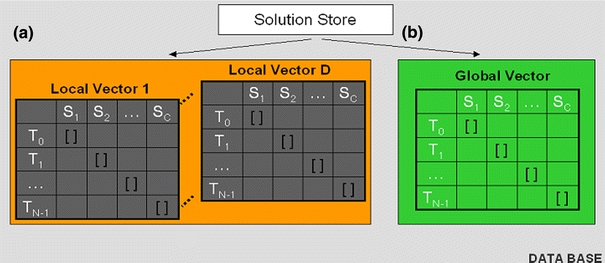
Local vectors and global vector solution store. There are D local vectors and one global vector

Global Vector

CytoSolve’s goal is to integrate or couple the computations of all the Models and dynamically compute the integrated model, O, as previously defined in Appendix A. The integrated solution for O is denoted as:

B3

where as before j references a molecular species with j = 1 to C, with C being the total number of unique molecular species across the union of all models M; and, n references the time step with n = 0 to N − 1, where N being total number of time steps.

The integrated solution is stored as shown in Fig. 9b. Each row of the Global Vector is computed using the formulation of the integrated solution.

Formulation of the Integrated Solution

This formulation is used to compute the integrated solution denoted in (B3). At each time step, each Model will have receive an input S _M,n and produce an output S _M,n+1. Since mass must be conserved, for each species j, the formulation calculates the production and consumption of species j, across all Models by:

B4

The integrated solution, at each time step n, for each species j, is evaluated as:

B5

At n = 0, the initial conditions are such that for all species:

B6

At each time step n, the Controller computes the Local Vectors for each Model. Equation (B5) is then used to compute the Global Vector at each time step n for each species j.

Appendix C

Structure of the Ontology Store

CytoSolve allows new models to be added to an ensemble through its ontology. Currently, the ontology is rudimentary using an ASCII file system. One set of files, in a Pathway Interface Document (PID) format, stores data on the specifics of each model. Another file contains a list of Unique Identifiers for resolving species name conflicts across models. During model registration, a PID file is created for each model. The format of the PID is show in Table 2.

Table 2.

Basic ontology PID format

Name of variable	Meaning
ModelName	The unique name of the model
ModelURL	The location on the Internet where the model executable code resides
Species	The number of species in the model
Species 1, Loc	The name of the first species (as used in the Model) and its location ID
Species 2, Loc	The name of the second species (as used in the Model) and its location ID.
…	…
Species n, Loc	The name of the nth species (as used in the Model) and its location ID

In Fig. 10 is a picture of an example PID file for a model called Model 1. The Loc is the location ID denoting which compartments the species appears in the cell. The species STAT1, for example, can appear in two locations. Loc ID “1” may denote the nucleus and Loc ID “2” may denote the mitochondrion, etc. Species need to be distinguished by their location. The MIRIAM standard was published which serves to provide a framework for model developers to provide a minimal set of information for defining biochemical models.18 Our basic ontology can take advantage of this emerging standard. Each model when it registers itself to be part of an ensemble creates a PID file.

Figure 10.

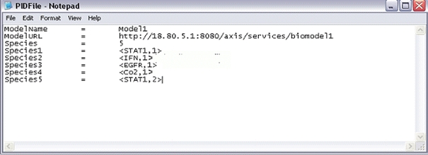
PID File example for storing CytoSolve’s representation of simple biological pathway model

There are some interesting challenges that can take place during registration of two different models. One example is if two species names are assigned the same name but mean something different or two species names are assigned different names but mean the same thing. The creators of SBMLMerge24 have identified this as a problem in the implementation of their tool to support semi-automatic source code merging of SBML model files. CytoSolve, includes as as a part of the basic ontology, a file containing a list of Unique Identifiers for mapping Unique Identifier # with a Species Name. This file is like a thesaurus. An example is shown in Table 3.

Table 3.

Unique Identifier file example

Unique Identifier #	Synonym
11231	Ca
11231	Calcium
11231	Ca+
11245	SOCS
…	…

Let us consider the case where two models have two different names for the exact same species. For example, suppose one model refers to a species called “Calcium” and another model refers to a species called “Ca+”. In Table 3, during registration, both of these species will point to Unique Identifier # 11231. The system will automatically resolve those species to be the same species internally. Prior to registering a new model, one can decide to use existing identifiers and names or add their own identifiers and name to the ontology. For example, let us say a developer has a species called “Cal” and that also refers to the same species as “Calcium” or “Ca+”, then the developer can update the ontology so 11231 also has an entry for “Cal” or they can adjust their species name to one of the existing synonyms.

Alternatively, let us consider the case of two models where the species name “CALCIUM” is assigned the same name in each model. When any model registers itself with the system, the PID file for that model is compared with other existing PID files and the Unique Identifier list. If CALCIUM is used in another model, then the system indicates that CALCIUM is currently being used by two other models, along with the Unique Identifier # for CALCIUM. If the author of that model believes that CALCIUM in fact refers to the same species, then no changes are required. If the model’s author believes that the species name should be different, then the onus is on the author to create a new Unique Identifier # and Species Name and resubmit.

The basic ontology of CytoSolve provides the Controller the basic knowledge to integrate species values across an ensemble of models. Currently, PID file creation and the Unique Identifier list maintenance and update is done manually; however, an automated process is under development to enable automatic comparison across models of species and reactions.

Appendix D

Sample Example of a Model and Input and Output Format for a Model

The purpose of this Appendix is to provide an example of a simple model, how CytoSolve interacts with the model, and how the model interacts with other models. Figure 11a shows a molecular pathway. This pathway contains five species with each species coded in a particular color. Each species interacts with other species as denoted by the arrows. Figure 11b shows the equivalent molecular pathway model of the same pathway. CytoSolve treats the model as a black box, concerned with its inputs and outputs. There are five (5) inputs to the model and five (5) outputs from the model, associated with the five species as indicated by color in Fig. 11b. The input to the model is the values of the species concentration at time step n and the output from the model is the values of the species concentration at time step n + 1.

Figure 11.

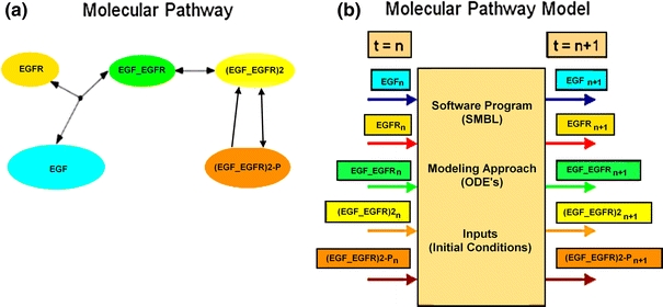
Simple example of a molecular pathway and model in CytoSolve. (a) Molecular pathway with five species and reactions. (b) Molecular pathway model with five inputs and five outputs of species concentrations at t = n and t = n + 1, respectively

The code within the “black box” of the model is not shielded even from CytoSolve. Thus, unlike monolithic systems, where model codes have to be linked together, with CytoSolve, there is no linking of model codes. Rather, at each time step, a model receives its inputs, executes, and returns its outputs. In Fig. 11b, the model format is in SBML, and the model’s mathematical approach is to use ODE’s. CytoSolve however is agnostic to the internal representation of the model. CytoSolve’s Controller processes the input and output streams across all models, as discussed in the “Computational Methodology” section to link and dynamically integrate solutions across all models to yield solutions for temporal changes in species concentrations.

Appendix E

Using CytoSolve

The first two basic requirements for use of the system are registering and logging in. There are three (3) main use cases of CytoSolve: Case I—Remote Mode; Case II—Local Mode; and, Case III—Combined Mode. During Remote Mode, the user can select models loaded on CytoSolve’s remote servers, and then integrate them. During Local Mode, the user simply downloads the local solver and combines and runs models resident on their local computer. During Combined Mode, the user can combine models resident on their local machines and with models resident on CytoSolve’s remote servers.

The initial steps in using CytoSolve for each mode vary. The initial steps for each mode are outlined in the sub-section “Initial Steps Across All Modes”. Thereafter, the usage steps are common across all modes as outlined in the sub-section “Common Steps Across Modes”.

Initial Steps Across All Modes

• I.
  Remote Model Case

  • Step 1—Select Remote Solving.
  • Step 2—Select Models to be Integrated. Iteratively, using the drop-down, individual models, which have been pre-registered and loaded onto the remote CytoSolve server(s) are selected.

To make models accessible for use by others, one simply loads up the model from the user interface to make it available for others to “see” and use. To create the original model itself, for example in SMBL, tools such as Cell Designer, MATLAB and others can be used.

• II.
  Local Model Case

  • Step 1—Select Local Solving.
  • Step 2—Download the Local Solver. Currently we support the SBML ODE solver, which can be downloaded to PC or MAC. Once the solver is downloaded, a README file provides instructions on how to install and initiate and run the solver.
  • Step 3—Select the Models to Run. Once the local solver is installed, one simply browses and selects the model(s) that one wishes to run and integrate locally.
• III. Combined Mode Case
  (Here it is assumed that the user has set up the Local Solver).

  • Step 1—Select Combined Solving.
  • Step 2—Select Models to be Integrated. Iteratively, using the drop-down, select individual models, which have been pre-registered and loaded onto the remote CytoSolve server(s) as well as the local models, which will appear on the drop down list.

Note: In this drop down list, CytoSolve lists models from the entire Biomodels.Net repository as well as any other models loaded by users of the system. If a local user wishes to make their model available for others to “see”, the user can simply upload their model into the CytoSolve system by entering the Remote Mode and doing so. Within the current web-based GUI, we are porting features from our non-web interface to enable users to simply register their local models and make CytoSolve aware of the model on their local personal computer, so no upload is necessary. However, some important network security issues need to be addressed, before that feature is released to the public, since CytoSolve will have direct access to the user’s local machine through the Web, in such cases.

Common Steps Across Modes

• Step A—Perform Pre-Checks (Align Models). Align models by executing pre-checks and determine duplicate species and reactions. User may be alerted to resolve species naming conflicts. These naming conflicts can be resolved manually or through auto alignment.

• Step B—Set Initial Conditions. Set the initial conditions for all species, spanning all models to be integrated.

• Step C—Execute. CytoSolve performs dynamic integration of the models selected.

• Step D—Display Data. Results from the integration can be viewed as graphs or the data, alternatively, can be downloaded for local analysis.

References

- 1.Aderem A. Systems biology: its practice and challenges. Cell. 2005;121:511–513. doi: 10.1016/j.cell.2005.04.020. [DOI] [PubMed] [Google Scholar]
- 2.Andersen DH. Compartmental Modeling and Tracer Kinetics. Berlin: Springer; 1983. [Google Scholar]
- 3.Barth M, Hennicker R, Kraus A, Ludwig M. DANUBIA: an integrative simulation system for global change research in the upper Danube basin. Cybern Syst. 2004;35:639–666. doi: 10.1080/01969720490499425. [DOI] [Google Scholar]
- 4.Bassingthwaighte JB, Chizeck HJ, Atlas LE, Qian H. Multiscale modeling of cardiac cellular energetics. Ann. N. Y. Acad. Sci. 2005;1047:395–424. doi: 10.1196/annals.1341.035. [DOI] [PMC free article] [PubMed] [Google Scholar]
- 5.Brooks, F. The Mythical Man Month: Essays in Software Engineering. Addison-Wesley, 1975.
- 6.Christensen, E., F. Curbera, G. Meredith, and S. Weerawarana (editors). Web services description language (WSDL) 1.1. W3C Note, 2001.
- 7.Eaves J, Godfrey W, Jones R. Apache Tomcat Bible. New York: John Wiley & Sons; 2003. [Google Scholar]
- 8.Ederer M, Gilles ED. Thermodynamically feasible kinetic models of reaction networks. Biophys. J. 2007;92(6):1846–1857. doi: 10.1529/biophysj.106.094094. [DOI] [PMC free article] [PubMed] [Google Scholar]
- 9.Gonzalez PP, et al. Cellulat: an agent-based intracellular signaling model. Biosystems. 2003;68(2–3):171–185. doi: 10.1016/S0303-2647(02)00094-1. [DOI] [PubMed] [Google Scholar]
- 10.Hood L, Heath JR, Phelps ME, Lin B. Systems biology and new technologies enable predictive and preventative medicine. Science. 2004;306:640–643. doi: 10.1126/science.1104635. [DOI] [PubMed] [Google Scholar]
- 11.Hucka M, et al. The systems biology markup language (SBML): a medium for representation and exchange of biochemical network models. Bioinformatics. 2003;19:524–531. doi: 10.1093/bioinformatics/btg015. [DOI] [PubMed] [Google Scholar]
- 12.Hunter P, Smith N, Fernandez J, Tawhai M. Integration from proteins to organs: the IUPS Physiome Project. Mech. Ageing Dev. 2005;126:187–192. doi: 10.1016/j.mad.2004.09.025. [DOI] [PubMed] [Google Scholar]
- 13.Ideker T, Lauffenburger D. Building with a scaffold: emerging strategies for high- to low-level cellular modeling. Trends Biotechnol. 2003;21(6):255–262. doi: 10.1016/S0167-7799(03)00115-X. [DOI] [PubMed] [Google Scholar]
- 14.Kholodenko BN, Demin OV, Moehren G, Hoek JB. Quantification of short term signaling by the epidermal growth factor receptor. J. Biol. Chem. 1999;274:30169–30181. doi: 10.1074/jbc.274.42.30169. [DOI] [PubMed] [Google Scholar]
- 15.Kitano H. Computational systems biology. Nature. 2002;420:206–210. doi: 10.1038/nature01254. [DOI] [PubMed] [Google Scholar]
- 16.Kitano H, Funahashi A, Matsuoka Y, Oda K. Using process diagrams for the graphical representation of biological networks. Nat. Biotechnol. 2005;23(8):961–966. doi: 10.1038/nbt1111. [DOI] [PubMed] [Google Scholar]
- 17.Le Novère N, et al. BioModels Database: a free, centralized database of curated, published, quantitative kinetic models of biochemical and cellular systems. Nucleic Acids Res. 2006;34(suppl 1):D689–D691. doi: 10.1093/nar/gkj092. [DOI] [PMC free article] [PubMed] [Google Scholar]
- 18.Le Novère N, et al. Minimum information requested in the annotation of biochemical models (MIRIAM) Nat. Biotechnol. 2007;23:1509–1515. doi: 10.1038/nbt1156. [DOI] [PubMed] [Google Scholar]
- 19.Liang, S. The Java Native Interface. Addison-Wesley, 1999.
- 20.Machne R, et al. The SBML ODE Solver Library: a native API for symbolic and fast numerical analysis of reaction networks. Bioinformatics. 2006;22:1406–1407. doi: 10.1093/bioinformatics/btl086. [DOI] [PubMed] [Google Scholar]
- 21.Mendes P, et al. Computational modeling of biochemical networks using COPASI. Methods Mol. Biol. 2009;500:17–59. doi: 10.1007/978-1-59745-525-1_2. [DOI] [PubMed] [Google Scholar]
- 22.Palsson BO, Price ND, Papin JA. Development of network-based pathway definitions: the need to analyze real metabolic networks. Trends Biotechnol. 2003;21:195–198. doi: 10.1016/S0167-7799(03)00080-5. [DOI] [PubMed] [Google Scholar]
- 23.Pillai S, et al. SOAP-based services provided by the European Bioinformatics Institute. Nucleic Acids Res. 2005;33:W25–W28. doi: 10.1093/nar/gki491. [DOI] [PMC free article] [PubMed] [Google Scholar]
- 24.Schulz, M., J. Uhlendorf, E. Klipp, and W. Liebermeister. SBMLmerge, a system for combining biochemical network models. Genome Inform. 17(1):62–71, 2006. [PubMed]
- 25.Snoep JL, Bruggeman F, Olivier BG, Westerhoff HV. Towards building the silicon cell: a modular approach. Biosystems. 2006;83:207–216. doi: 10.1016/j.biosystems.2005.07.006. [DOI] [PubMed] [Google Scholar]
- 26.Tomita M, et al. E-CELL: software environment for whole-cell simulation. Bioinformatics. 1999;15:72–84. doi: 10.1093/bioinformatics/15.1.72. [DOI] [PubMed] [Google Scholar]
- 27.Vangheluwe, H. DEVS as a common denominator for multi-formalism hybrid modeling. In: Proceedings of the IEEE International Symposium on Computer Aided Control System Design, 2000, pp. 129–134.
- 28.Webb K, White T. UML as a cell and biochemistry modeling language. Biosystems. 2005;80:283–302. doi: 10.1016/j.biosystems.2004.12.003. [DOI] [PubMed] [Google Scholar]
- 29.Zeigler B. Hierarchical modular discrete-event modelling in an object-oriented environment. Simulation. 1987;49:219–230. doi: 10.1177/003754978704900506. [DOI] [Google Scholar]