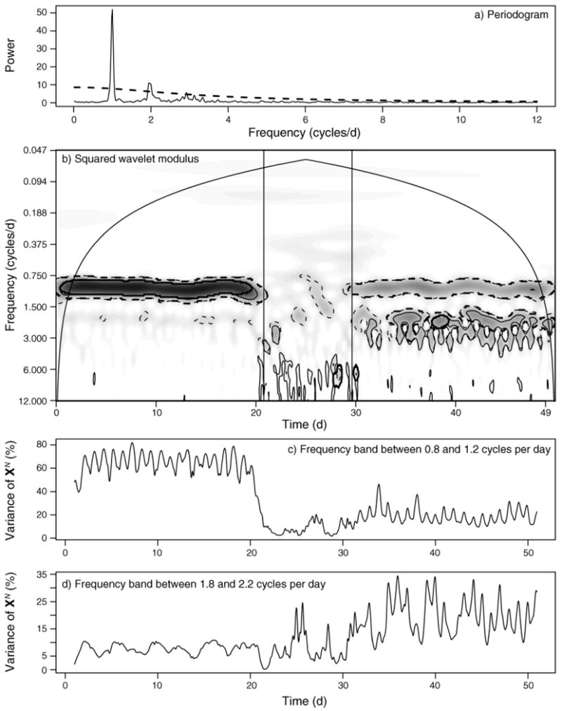
Fig. 4.

Frequency and time–frequency analyses of a simulated individual movement trajectory over 50 days sampled at Δt = 1 hour. The daily behavioral sequence (with mi defined in Methods: Stochastic movement model) was SK = {m1, m2, m3, m2} and EK = {6, 6, 6, 6}, corresponding to equal times of rest, feed, taxis, feed for the first 20 days, followed by randomly chosen behavioral modes with expected temporal duration τk = 1 hour for the middle 10 days, and ending with crepuscular activity defined as SK = {m1, m3, m2, m1, m2, m3} with EK = {4, 4, 4, 4, 4} corresponding to equal expected durations of rest, taxis, walk, rest, walk, taxis, during the final 20 days. (a) The normalized smoothed periodogram shows peaks different from white (constant value of 1) or red (dashed line) noise null models, suggesting cyclic behavior. (b) Contoured squared wavelet modules values (smaller values are given by whiter colors and larger values by darker colors). Using 1000 simulated step-length time series based on the white and red noise null models, we calculated the bootstrapped 95th percentile significant patches, delineated by thin dashed and solid lines, respectively; significant patches remaining from an areawise test (see Methods: Fourier and wavelet transformation) are delineated by thick dashed and solid lines for the white and red noise null models, respectively. The cone of influence is delineated by the arched solid black line. Panels (c) and (d) show the time series of the percentage variance explained by frequency bands around (c) ω = 1 cycle/day and (d) ω = 2 cycles/day, where XN is the length N time series of movement velocities, defined in Methods: Fourier and wavelet transforms.
