Abstract
Saw marks on bone have been routinely reported in dismemberment cases. When saw blade teeth contact bone and the bone is not completely sawed into two parts, bone fragments are removed forming a channel or kerf. Therefore, kerf width can approximate the thickness of the saw blade. The purpose of this study is to evaluate 100 saw kerf widths in bone produced by ten saw types to determine if a saw can be eliminated based on the kerf width. Five measurements were taken from each of the 100 saw kerfs to establish an average thickness for each kerf mark. Ten cuts were made on 10 sections of bovine bone, five with human-powered saws and five with mechanical-powered saws. The cuts were examined with a stereoscopic microscope utilizing digital camera measuring software. Two statistical cumulative logistic regression models were used to analyze the saw kerf data collected. In order to estimate the prediction error, repeated stratified cross-validation was applied in analyzing the kerf mark data. Based on the two statistical models used, 70–90% of the saws could be eliminated based on kerf width.
Keywords: Tool marks, Saw marks, Kerf mark analysis, Dismemberment
Introduction
Postmortem dismemberment cases, sometimes referred to in the media as corpse mutilation, abuse of corpse or criminal dismemberment, present a challenge to investigators attempting to identify the tool used in the dismemberment [1]. If multiple tools are recovered, examinations could be conducted to link or eliminate each of the tools used in the dismemberment. Postmortem dismemberment is typically accomplished with a knife, axe, saw or a combination of these cutting tools. When these types of cutting tools are used, they can leave tool marks on cartilage and bone. Sometimes these marks can be used to match or eliminate the tool [2, 3]. Even if the cutting tool cannot be matched or eliminated, an examination of the tool marks can provide some information about the general characteristics of the tool [4, 5].
Cutting tools leave two types of characteristics, individual and class, that can be used to analyze tool marks. Individual characteristics are random imperfections along the leading edge of the cutting tool that produce striations on a substrate; therefore, these striations can be used to match a cutting tool to a specific tool mark. Class characteristics include similarities that can place the tool in a category or eliminate it from a group [6–8]. For example, a saw blade that is 6.350 mm in thickness could be eliminated from a cut mark that is 3.175 mm in width. Moreover, in any form of physical comparative analysis, class characteristics are examined first to determine if they are the same or similar. If a tool can be eliminated based on a difference in class characteristics, it is not necessary to search for individual characteristics. However, if the class characteristics are the same or similar, a physical match or elimination can be achieved based on the agreement or disagreement of individual characteristics [9].
When saws are used to cut bone, they sometimes leave marks known as false starts. False starts occur when the saw blade comes into contact with bone briefly, removes some of the bone but then stops, skips or restarts in a new position usually close to the initial cut and continues to cut the bone [10]. The characteristic examined in this study was the kerf width of a saw cut into compact bone. The kerf mark widths were measured to determine which possible saw blade could be eliminated based on the kerf width.
Methods
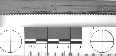
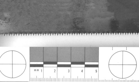
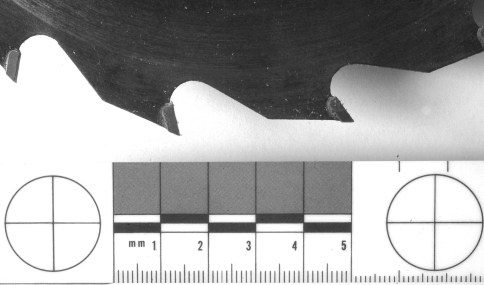
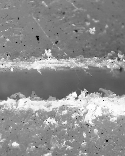
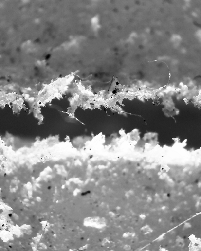
Ten sections of bovine bone were cut into ~22.86 cm by ~5.08 cm sized pieces and used as a substrate to collect kerf marks from five human-powered and five mechanical-powered saws. The human-powered saws included: a hand saw, hack saw, meat saw, bow saw and molding cut-off saw. The mechanical-powered saws included: a reciprocating saw, circular saw, cut-off saw, portable band saw, and jig saw. Of the mechanical-powered saws, the circular saw, cut-off saw and portable band saw used cutting blades with a rotating motion. The reciprocating saw and jig saw used cutting blades with a reciprocating motion. Kerf marks were produced on the diaphyseal sections by sawing into the cortical bone with each of the saws. The depth of each saw cut was approximately ½ the thickness of the compact bone. Figures 1, 3, 5, 7, 9, 11, 13, 15, 17, and 19 illustrate the saw blades used and Figs. 2, 4, 6, 8, 10, 12, 14, 16, 18, and 20 illustrate the kerf for each of the blades respectively.
Fig. 1.
Portable band saw blade
Fig. 3.
Hack saw blade
Fig. 5.
Bow saw blade
Fig. 7.
Molding cut-off blade
Fig. 9.
Meat saw blade
Fig. 11.
Jig saw blade
Fig. 13.
Hand saw blade
Fig. 15.
Reciprocating blade
Fig. 17.
Circular saw blade
Fig. 19.
Cut-off saw blade
Fig. 2.
Portable band saw blade kerf
Fig. 4.
Hack saw blade kerf
Fig. 6.
Bow saw blade kerf
Fig. 8.
Molding cut-off blade kerf
Fig. 10.
Meat saw blade kerf
Fig. 12.
Jig saw blade kerf
Fig. 14.
Hand saw blade kerf
Fig. 16.
Reciprocating blade kerf
Fig. 18.
Circular saw blade kerf
Fig. 20.
Cut-off saw blade kerf
Dial calipers were used to measure the thickness of each saw blade. Before recording measurements, steps were taken to ensure the dial calipers were operating properly. First, the dial caliper jaws were closed and the pointer setting was at “0.” Second, using the thumbwheel, the dial caliper jaws were opened to the maximum distance and then third, they were closed. When closed, the pointer setting returned to “0.” The thickness of the blade and the teeth are reported in Table 1. The saw kerf and teeth width characteristics are reported in Table 2. The width of the teeth on mechanical-powered saw and human-powered saws can be the same size as the blade or wider than the blade. The teeth on the blades from the human-powered saws ranged from 0.025 mm to .0457 mm in size while the teeth on the mechanical saws ranged from 0.025 mm to 0.762 mm in size.
Table 1.
Blade and teeth width (mm) characteristics for non-powered and electrical saws
| Saw types | Blades | Teeth | Differences |
|---|---|---|---|
| Hand saw | 0.940 | 1.400 | 0.460 |
| Hack saw | 0.610 | 0.660 | 0.050 |
| Meat saw | 0.635 | 0.914 | 0.279 |
| Bow saw | 0.889 | 0.914 | 0.025 |
| M. cut-off | 0.635 | 0.889 | 0.254 |
| Reciprocating | 1.016 | 1.397 | 0.381 |
| Skill saw | 1.397 | 2.083 | 0.686 |
| Cut-off saw | 1.905 | 2.667 | 0.762 |
| P. band saw | 0.635 | 0.660 | 0.025 |
| Jig saw | 0.940 | 1.143 | 0.203 |
Table 2.
Saw kerf and teeth width characteristics (mm) for non-powered and electrical saws
| Saw types | Kerf range | Average kerf | Teeth width | Difference between av. kerf and teeth |
|---|---|---|---|---|
| Hand saw | 1.397–1.829 | 1.410 | 1.397 | 0.013 |
| Hack saw | 0.711–1.020 | 0.813 | 0.660 | 0.153 |
| Meat saw | 1.067–1.245 | 1.118 | 1.067 | 0.051 |
| Bow saw | 0.914–1.041 | 0.965 | 0.914 | 0.051 |
| M. cut-off | 0.889–1.143 | 0.991 | 0.889 | 0.102 |
| Reciprocating | 1.397–1.575 | 1.448 | 1.397 | 0.051 |
| Skill saw | 2.210–3.150 | 2.718 | 2.082 | 0.636 |
| Cut-off saw | 2.667–2.870 | 2.794 | 2.667 | 0.127 |
| P. band saw | 0.660–0.864 | 0.737 | 0.660 | 0.077 |
| Jig saw | 1.270–1.473 | 1.346 | 1.143 | .203 |
Ten saw types were used to cut kerfs into ten separate sections of bone. One saw type was used on each bone section to produce ten kerfs. Each kerf was examined with a stereoscopic boom microscope equipped with a digital camera and measuring software. Next, the digital camera measuring software was calibrated according to the manufacturer’s instructions using a calibration disk with a 7,500 μm black calibration circle that was supplied with the digital camera and measuring software. A magnification of 20× was selected to examine each of the kerfs. Five measurements were taken from each of the kerfs. The measurement data was then subjected to statistical analysis for comparison of saw kerf widths and saw blade thicknesses.
Statistical analysis
Two cumulative logit models using Statistical Analysis System (SAS) software were used to analyze the data in this study [11, 12]. In statistics, logit regression is proposed for prediction of the probabilities of events. Logit models provide estimated probabilities given the realization of covariates compared with statistical descriptive analysis such as mean, median, standard deviation, interquartile range and range. Therefore, the logit models were used to indicate the likelihood of similar categories of saw types. A baseline-category logit model was not used for three reasons. First, as suggested by Fig. 1, the average kerf width is an indicator of the saw type, and incorporating the order of kerf widths improves the accuracy of the model. Second, there is one slope for each covariate which facilitates interpreting the effect of the covariate and provides the proportional odds property needed for analysis. Lastly, in analyzing the kerf data, the quasi-complete separation problem for the data was avoided.
The first logit model considered kerf width only and no other saw information. Model #1 is
 |
where the covariate x is the kerf width and j is the ascending order of the 10 saw kerf widths (Table 3). The y axis in Model #1 represents the probability of saws based on kerf widths. The SAS results in Table 3 suggest the average kerf width is significant compared to the kerf width of other saws with a P-value less than 0.01%.
Table 3.
SAS results for the cumulative regression Model #1
| Testing global null hypothesis: BETA = 0 | |||||
|---|---|---|---|---|---|
| Test | Chi-square | DF | Pr > ChiSq | ||
| Likelihood ratio | 241.7532 | 1 | <0.0001 | ||
| Score | 78.1015 | 1 | <0.0001 | ||
| Wald | 68.7759 | 1 | <0.0001 | ||
| Parameter | DF | Estimate | Standard error | Wald Chi-square | Pr > ChiSq |
|---|---|---|---|---|---|
| Intercept 1 | 1 | 11.8983 | 1.6204 | 53.9194 | <0.0001 |
| Intercept 2 | 1 | 13.9035 | 1.7733 | 61.4725 | <0.0001 |
| Intercept 3 | 1 | 15.4594 | 1.8966 | 66.4385 | <0.0001 |
| Intercept 4 | 1 | 17.0854 | 2.0444 | 69.8408 | <0.0001 |
| Intercept 5 | 1 | 19.5395 | 2.4128 | 65.5813 | <0.0001 |
| Intercept 6 | 1 | 21.9773 | 2.6717 | 67.6682 | <0.0001 |
| Intercept 7 | 1 | 23.7759 | 2.7845 | 72.9106 | <0.0001 |
| Intercept 8 | 1 | 30.9098 | 4.3305 | 50.9476 | <0.0001 |
| Intercept 9 | 1 | 44.2137 | 5.3890 | 67.3120 | <0.0001 |
| Kerf mean (mm) | 1 | 15.8759 | 1.9143 | 68.7759 | <0.0001 |
Analysis of maximum likelihood estimates: 
The second logit model considered the kerf widths and saw teeth widths. Model #2 is
 |
where x 1 is the kerf width and x 2 is the saw tooth width. The y axis in model 2 represents the probability of kerf widths for the middle sections. The SAS results in Table 4 indicate the P-value is less than 0.01%; thus, the hypothesis that both covariates are negligible is not rejected. Therefore, the maximum likelihood estimates are significant.
Table 4.
SAS results for the cumulative regression Model #2
| Testing global null hypothesis: BETA = 0 | |||||
|---|---|---|---|---|---|
| Test | Chi-square | DF | Pr > ChiSq | ||
| Likelihood ratio | 351.6629 | 2 | <0.0001 | ||
| Score | 82.6585 | 2 | <0.0001 | ||
| Wald | 28.6652 | 2 | <0.0001 | ||
| Parameter | DF | Estimate | Standard error | Wald Chi-square | Pr > ChiSq |
|---|---|---|---|---|---|
| Intercept 1 | 1 | 32.7390 | 6.5963 | 24.6339 | <0.0001 |
| Intercept 2 | 1 | 38.5349 | 8.1150 | 22.5493 | <0.0001 |
| Intercept 3 | 1 | 43.2165 | 8.9154 | 23.4971 | <0.0001 |
| Intercept 4 | 1 | 45.1196 | 9.0023 | 25.1202 | <0.0001 |
| Intercept 5 | 1 | 51.4665 | 10.6254 | 23.4615 | <0.0001 |
| Intercept 6 | 1 | 61.6239 | 12.8314 | 23.0647 | <0.0001 |
| Intercept 7 | 1 | 67.0395 | 13.7036 | 23.9328 | <0.0001 |
| Intercept 8 | 1 | 85.7253 | 798.4 | 0.0115 | 0.9145 |
| Intercept 9 | 1 | 118.9 | 29.4648 | 16.2826 | <0.0001 |
| Kerf mean (mm) | 1 | 12.7198 | 3.6484 | 12.1548 | 0.0005 |
| Teeth | 1 | 34.6266 | 9.4667 | 13.3791 | 0.0003 |
Analysis of maximum likelihood estimates: 
Results
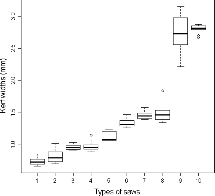
Figure 21 shows the boxplots of the kerf widths from the ten saws considered. When the kerf width is approximately 2.6 mm, the probability that the saw is a cut-off saw or a circular saw is approximately 0.50. It suggests that the cut-off saw and circular saw share similar medians; however, the kerf widths for the circular saw are more varied than the cut-off saw. This variation is possibly due to single or multiple factors. Some factors that could account for the differences in range of widths between the two saws are hand, wrist or arm movement while sawing which may affect the lateral movement of the blade, cutting rate, and blade vibration. Also, wear on the bearings could account for differences in the range of widths between kerfs produced by the two saws. The cut-off saw is attached to a steel frame and the saw movement is controlled by a hinge. Figure 1 suggests that there is a linear pattern among the other eight saws.
Fig. 21.
Boxplot of kerf widths. 1. Portable band saw, 2. Hack saw, 3. Bow saw, 4. Molding cut-off saw, 5. Meat saw, 6. Jig saw, 7. Reciprocating saw, 8. Hand saw, 9. Circular saw, 10. Cut-off saw. (For boxplot values, the top line represents the maximum width, next down the 3rd quartile, median, 1st quartile and lastly the minimum width. Also some boxplots have an outlier which is indicated by “O”)
In order to estimate the prediction error of the models, repeated stratified tenfold cross-validations were conducted. Therefore, regular cross-validation might not be sufficient, while repeated cross-validation provides more evidence about the prediction error of the models.
Tables 5 and 6 contain the simulation results of the repeated stratified 10-fold cross-validation, where Table 5 is generated from Model #1 and Table 6 is generated from Model #2. The simulation in R was run with a random seed number 68 to ensure that the results were reproducible. The replication time was 100.
Table 5.
Prediction results for Model #1 using stratified 10-fold cross validation with 100 replications
| Saw type | Predicted from Model #1 |
|---|---|
| Hand saw | Jig saw (22%) reciprocating (30%) and hand saw (48%) |
| Hack saw | Portable band (39%) hack saw (35%) bow saw (19%) and molding cut-off (7%) |
| Meat saw | Meat saw (89%) and jig saw (11%) |
| Bow saw | Bow saw (54%) and molding cut-off saw (46%) |
| Molding cut off | Hack saw (8%) bow saw (52%) molding cut-off saw (25%) and meat saw (15%) |
| Reciprocating | Jig saw (5%) reciprocating saw (60%) hand saw (35%) |
| Skill saw | Skill saw (60%) and cut off-saw (40%) |
| Cut-off saw | Skill saw (31%) and cut off-saw (69%) |
| Portable band | Portable band saw (76%) and hack saw (24%) |
| Jig saw | Jig saw (82%) reciprocating saw (12%) hand saw (6%) |
Table 6.
Prediction results for Model #2 using stratified 10-fold cross validation with 100 replications
| Saw type | Predicted from Model #2 |
|---|---|
| Hand saw | Reciprocating (52%) and hand saw (48%) |
| Hack saw | Portable band (39%) hack saw (61%) |
| Meat saw | Meat saw (100%) |
| Bow saw | Bow saw (34%) and molding cut-off saw (47%) meat saw (19%) |
| Molding cut off | Bow saw (83%) molding cut-off saw (10%) and meat saw (7%) |
| Reciprocating | Reciprocating saw (65%) hand saw (35%) |
| Skill saw | Skill saw (100%) |
| Cut-off saw | Cut off-saw (100%) |
| Portable band | Portable band saw (88%) and hack saw (12%) |
| Jig saw | Jig saw (100%) |
Comparisons were made between the two statistical logit models. Model #1 was used to calculate possible saw blade eliminations and likelihood similarities to other saws based on kerf width measurements. This data is summarized in Table 5. Based on this model, there is a 48% chance that the hand saw kerf originated from the hand saw, a 22% chance that the hand saw kerf was from the jig saw and a 30% chance that it was from the reciprocating saw. The least accurate predictions for Model #1 were with the hack saw and molding cut-off saw. There was only a 35% chance that the kerf from the hack saw originated from the hack saw and a 39% chance that kerf was from the portable band saw. For the molding cut-off saw, there was a 25% chance that the molding cut-off saw kerf originated from the molding cut-off saw. There was a 52% chance that the molding cut-off saw kerf was from the bow saw.
Model #2 was used to calculate possible saw blade eliminations and likelihood similarities to other saws using kerf widths as well as saw teeth widths. This data is summarized in Table 6. Using this model, all saws were eliminated from the meat saw, circular saw, cut-off saw and jig saw. However, the bow saw kerf was predicted to have a 34% chance of originating from the bow saw and a 47% chance of originating from the molding cut-off saw. Also, the molding cut-off saw kerf width had only a 10% chance of originating from the molding cut-off saw and an 83% chance of originating from the bow saw. In summary, statistical Model #2 is a more accurate model for predicting the possible saw types based on kerf widths used in this study.
The logit models have limitations when some kerf marks cannot be separated. Therefore, the logistic regression provides an estimated probability of each category and it is possible that two or more categories may share similar probabilities given a specific covariate value, namely, the kerf width. When the categories are not separable, there may be a higher false probability rate. For example, in Model #1 the bow saw and molding cut-off saw present limitations due to similarities of the kerf marks. Also, in Model #2 the kerf marks produced by the bow saw and molding cut-off saw present limitations because they cannot be separated. However, the logit models provide likelihoods for each saw type given the limitations.
Discussion
Saw characteristics affecting the kerf width and bone surface adjacent to the kerf include style and design of the teeth, width of the teeth, teeth per inch (tpi), degree of wear on the teeth, saw cutting speed, blade vibration, defects in the blade or erratic sawing motion. Also, a worn bushing in mechanical-powered saws can affect kerf widths. With the exception of band saw type saws, mechanical-powered saws generally require thicker blades than human-powered saws due to saw power and operating speeds. Consequently, these saws produce broader kerf widths than human-powered saws [13–15].
Additionally, fire can alter tool marks on bone. For example, fire can result in a loss of structural integrity causing bone to easily fracture. It can obscure some of the individual and class characteristics and also cause shrinkage in bone [16–18]. Bone shrinkage will affect saw blade predictions based on kerf widths.
Key Points
Postmortem dismemberment cases are sometimes referred to in the media as corpse mutilation, abuse of corpse and criminal dismemberment.
The style and design of the teeth, width of the teeth, teeth per inch (tpi), degree of wear on the teeth, saw cutting speed, blade vibration, defects in the blade, and erratic sawing motion are factors that affect the kerf. Accurate microscopic measurements may be more difficult when the kerf shoulders are fibrous.
Analyzing kerf mark measurements can be an effective method for predicting and eliminating possible saw blades by comparing the width of the blade to the width of the kerf.
Statistical model #2 provides more accurate predictions of possible saw types based on kerf widths than Model #1. However, both models have limitations; when the categories cannot be separated, there may be higher false probability rates.
The boxplot of kerf widths in Fig. 21 provides the investigator with a reference guide for eliminating saw types based on kerf width range calculations.
Open Access
This article is distributed under the terms of the Creative Commons Attribution Noncommercial License which permits any noncommercial use, distribution, and reproduction in any medium, provided the original author(s) and source are credited.
Contributor Information
James A. Bailey, Phone: +1-910-8154047, Email: james.bailey@mnsu.edu, Email: jbailey30@ec.rr.com
Yishi Wang, Email: Wangy@uncw.edu.
Frank R. W. van de Goot, Email: FRW.Goot@vumc.nl
Reza R. R. Gerretsen, Email: r.gerretsen@nfi.minjus.nl
References
- 1.Saul FP, Saul JM, Symes SA. The lady in the box. Proc Am Acad For Sci. 2005;11:300. [Google Scholar]
- 2.Saville PA, Hainsworth SV, Rutty GN. Cutting crime: the analysis of the “uniqueness” of saw marks on bone. Int J Legal Med. 2007;121.5:349–357. doi: 10.1007/s00414-006-0120-z. [DOI] [PubMed] [Google Scholar]
- 3.Bonte W. Tool marks in bones and cartilage. J Forensic Sci. 1975;20:315–323. [PubMed] [Google Scholar]
- 4.Rowe WF. Forensic science: an introduction to scientific and investigative techniques. In: James SH, Nordby JJ, editors. Firearms and toolmarks examinations. Boca Raton, Florida: CRC Press; 2003. pp. 327–355. [Google Scholar]
- 5.Bertino AJ, Bertino PN. Forensic science: fundamentals and investigations. Mason, Ohio: South-Western Cengage Learning; 2008. pp. 470–474. [Google Scholar]
- 6.Hueske EE. Firearms and toolmarks. In: Mozayani A, Noziglia C, editors. Forensic laboratory handbook: procedures and practice. Towowa, NJ: Humana Press Inc; 2006. pp. 143–145. [Google Scholar]
- 7.Nickell J, Fischer JF. Crime science: methods of forensic detection. Lexington: University Press of Kentucky; 1999. pp. 154–157. [Google Scholar]
- 8.Davis JE. An introduction to tool marks, firearms and the striagraph. Springfield: Charles C Thomas; 1958. pp. 7–25. [Google Scholar]
- 9.Grybowski R, Miller J, Moran B, Murdock J, Nichols R, Thompson R. Firearm/toolmark identification: passing the reliability test under federal and state evidentiary standards. AFTE J. 2003;35:209–221. [Google Scholar]
- 10.Symes SA, Berryman HE, Smith OC. Saw marks in bone: introduction and examination of residual kerf contour. In: Reichs KJ, editor. Forensic osteology: advances in the identification of human remains. 2. Springfield: Charles C Thomas; 1998. pp. 393–395. [Google Scholar]
- 11.Agresti A. Categorical data analysis. 2. Hoboken, N.J: Wiley; 2002. pp. 165–266. [Google Scholar]
- 12.Stokes ME, Davis CS, Koch GG. Categorical data analysis using the SAS system. 2. Cary, NC: SAS Institute Inc; 2003. pp. 181–240. [Google Scholar]
- 13.Freas L. Assessment of saw-blade wear patterns and wear-related features of the kerf wall. Proc Am Acad For Sci. 2004;10:303–304. [Google Scholar]
- 14.Freas L. Scanning electron microscopy of saw marks in bone: assessment of wear-related features of the kerf wall. Proc Am Acad For Sci. 2006;12:296. doi: 10.1111/j.1556-4029.2010.01468.x. [DOI] [PubMed] [Google Scholar]
- 15.Symes SA, Kroman AM, Thurston Myster SM, Rainwater CW, Matia JJ. Anthropological saw mark analysis on bone: what is the potential of dismemberment interpretation? Proc Am Acad For Sci. 2006;12:301. [Google Scholar]
- 16.Marciniak S. A preliminary assessment of the identification of saw marks on burned bone. J Forensic Sci. 2009;54.4:779–785. doi: 10.1111/j.1556-4029.2009.01044.x. [DOI] [PubMed] [Google Scholar]
- 17.Ubelaker DH. The forensic evaluation of burned skeletal remains: a synthesis. For Sci Int. 2009;183:1–5. doi: 10.1016/j.forsciint.2008.09.019. [DOI] [PubMed] [Google Scholar]
- 18.Pope EJ, Symes SA, Smith OC. Burning observations of the head: an experimental model. Proc Am Acad For Sci. 2002;8:225–226. [Google Scholar]


