Metal artifact reduction in x-ray computed tomography (CT) by constrained optimization

Abstract

Purpose: The streak artifacts caused by metal implants have long been recognized as a problem that limits various applications of CT imaging. In this work, the authors propose an iterative metal artifact reduction algorithm based on constrained optimization.

Methods: After the shape and location of metal objects in the image domain is determined automatically by the binary metal identification algorithm and the segmentation of “metal shadows” in projection domain is done, constrained optimization is used for image reconstruction. It minimizes a predefined function that reflects a priori knowledge of the image, subject to the constraint that the estimated projection data are within a specified tolerance of the available metal-shadow-excluded projection data, with image non-negativity enforced. The minimization problem is solved through the alternation of projection-onto-convex-sets and the steepest gradient descent of the objective function. The constrained optimization algorithm is evaluated with a penalized smoothness objective.

Results: The study shows that the proposed method is capable of significantly reducing metal artifacts, suppressing noise, and improving soft-tissue visibility. It outperforms the FBP-type methods and ART and EM methods and yields artifacts-free images.

Conclusions: Constrained optimization is an effective way to deal with CT reconstruction with embedded metal objects. Although the method is presented in the context of metal artifacts, it is applicable to general “missing data” image reconstruction problems.

INTRODUCTION

Streak artifacts from high attenuation objects are a common problem in CT. This type of artifacts typically occurs from metallic implants such as dental fillings, hip prostheses, implanted marker bins, and branchy-therapy seeds. The artifacts not only blur the CT images and lead to inaccuracies in diagnosis, but also make the delineation of anatomical structures intractable, which is important in image-guided intervention procedures. Mathematically, the artifacts originate from the dark shadows in the measured sinogram due to the strong attenuation of the metal objects when x rays pass through them. These “metal shadows” provide little information for image reconstruction. How to deal with “missing data” is the essence of metal artifacts removal in reconstruction.

In the past three decades, numerous methods have been proposed to tackle the problem described above. These methods can generally be categorized into two classes. One is to identify the metal-contaminated region in the projection space and then fill in the missing data by using different interpolation schemes^{1, 2, 3} based on the uncontaminated projection data. CT images are then reconstructed from the completed projection data by analytical FBP-type algorithms. The interpolation-based algorithms can make unrealistic assumptions about the missing data, leading to prominent errors in the reconstructed images. Alternatively, metal artifacts are reduced by using model-based iterative reconstruction algorithms.^{4, 5, 6} The metal shadows are either manually or automatically segmented in the projection domain and iterative reconstruction is applied to better interpret the regions with incomplete projection database on some physical considerations. Compared to analytical reconstruction algorithms, an iterative technique more effectively utilizes prior knowledge of the image physics, noise properties, and imaging geometry of the system and thus can yield improved images. The performance of the method, however, may suffer from the inaccuracy of the metal object segmentation in the projection space.⁷ There are also a few case-by-case techniques to reduce metal artifacts,^{8, 9, 10, 11, 12, 13, 14} but a systematic approach is highly desirable.

A necessary step to ensure the success of iterative CT scan is to know about the shape and location and sometimes even the attenuation coefficients¹⁵ of the metal objects in image domain. We have recently proposed an image reconstruction method capable of autoidentifying the shape and location of metallic object(s) in the image space^{16, 17, 18} based on a penalized weighted least-squares (PWLS) method. The yielded binary image contains only metal and background and a forward projection of the image to the projection space provides accurate information of the metal corrupted projection data. In this work, we develop a constrained optimization method to effectively utilize this information to determine the tissue density distribution in the remaining part of the patient being scanned.

The statistics-based iterative reconstruction algorithms are usually formulated as unconstrained optimization models that minimize or maximize a cost function, constructed from noise characteristics of the measured data. There are usually two terms in the objective function: A data fidelity term and a regularization term that uses prior information to regularize the solution. Such a formulation is sensible for fully sampled tomographic systems where a unique image that minimizes the data-fidelity-objective function exists.¹⁹ However, when part of the projection data is missing in the form of metal shadows, there is, in general, no unique solution of the data-fidelity-objective function. In this situation, it is natural to use a constrained optimization model, where data fidelity becomes an inequality constraint to determine the feasible set of images that agree with the available measurement data within a specified tolerance, while image regularity is converted to the objective function and is used to select an optimal image out from the feasible set. The constrained optimization formulation is also flexible and allows easy incorporation of other constraints such as image positivity, extreme values, and bound on roughness.

In this work, we will first describe the image reconstruction procedure to identify metal object(s) in the projection domain. The constrained optimization model that reconstructs image with metal-shadow-excluded projection data, as well as the penalized smoothness (PS) objective function and the strategy to solve the optimization problem, will be introduced in Sec. 2. In Sec. 3, evaluation of the proposed algorithm is presented using a digital quality assurance (QA) phantom and an experimental QA phantom, followed by discussions and conclusions in Sec. 4.

METHODS AND MATERIALS

Metal localization and reconstruction

We use an image intensity threshold-based reconstruction method to identity the metal object(s) from the x-ray projection data. When a metal object is present in a patient, an image can be divided into two prominent components and the task here is to find the boundary between the high and low density regions from the projection data. An iterative image reconstruction algorithm based on the PWLS criterion is implemented to accomplish the goal.

Mathematically, the PWLS criterion can be written as^{20, 21}

$$\Phi \left(\stackrel{⃑}{\mu }\right)={\left(\stackrel{⃑}{p}-A\stackrel{⃑}{\mu }\right)}^{\prime }{\Sigma }^{-1}\left(\stackrel{⃑}{p}-A\stackrel{⃑}{\mu }\right)+\widehat{\beta }R\left(\stackrel{⃑}{\mu }\right).$$ (1)

The first term in Eq. 1 is the weighted least-squares criterion, where $\stackrel{⃑}{p}$ is the vector of log-transformed projection measurements and $\stackrel{⃑}{\mu }$ is the vector of attenuation coefficients to be reconstructed. Symbol ^′ denotes the transpose operator. Operator A represents the system or projection matrix. The projection data $\stackrel{⃑}{p}$ and the attenuation map $\stackrel{⃑}{\mu }$ are related by $\stackrel{⃑}{p}=A\stackrel{⃑}{\mu }$. Thus, the least-squares criterion actually reflects the data fidelity. Σ is a diagonal matrix with the ith element of ${\sigma }_i^2$, i.e., an estimate of the variance of repeatedly measured ${\stackrel{⃑}{p}}_i$ at detector bin i which can be estimated from the measured projection data according to a mean-variance relationship of projection data.^{22, 23} The second term in Eq. 1 is a smoothness penalty or a prior constraint, where $\widehat{\beta }$ is the smoothing parameter that controls relative contribution from the measurement and prior constraint. The second term in Eq. 1 enforces a roughness penalty on the solution. In order to reconstruct binary image (i.e., metals and normal tissues), we design a special quadratic penalty term in Eq. 2 by introducing a gradient-controlled parameter c_jm. The form of the new penalty is expressed as:

$$R\left(\stackrel{⃑}{\mu }\right)={\stackrel{⃑}{\mu }}^{\prime }R\stackrel{⃑}{\mu }=\frac{1}{2}\sum _j\sum _{m∊N_j}{c}_{jm}{w}_{jm}{\left({\mu }_j-{\mu }_m\right)}^2,$$ (2)

where

$$c_{jm}=\{\begin{array}{cc}0& \left|{\mu }_j-{\mu }_m\right|\ge \varphi \\ 1& \left|{\mu }_j-{\mu }_m\right|<\varphi \end{array}\phantom{\}}.$$ (3)

Where the index j runs over all image elements in the image domain, N_j represents the set of neighbors of the jth image pixel. The parameter w_jm was set to 1 for first-order neighbors and $1∕\sqrt{2}$ for second-order neighbors. Note that without parameter c_jm, Eq. 2 is exactly a quadratic penalty with equal weights for neighbors of the same distance used widely for iterative image reconstruction.^{20, 21, 25} The idea behind Eq. 3 is that regularization is only applied to neighbors which have gradient smaller than the threshold ϕ, while the regularization between neighbors will be suppressed if magnitude of gradient between them is larger the threshold ϕ. The difference of linear attenuation coefficients between metal and normal structures is usually larger than that between different structures. By setting a proper ϕ, the regularization term of the smoothness constraint will be applied only within the metal objects or the patient structures. In practice, the parameter ϕ is empirically determined. We set $\widehat{\beta }=1\times {10}^{10}$ and ϕ=0.06 in the digital phantom simulations and $\widehat{\beta }=1\times {10}^{10}$ and ϕ=0.06 in the experimental studies.

The Gaussian–Seidel updating strategy is used for the minimization of Eq. 1.^{16, 17} Once the image is reconstructed, a thresholding operation is applied to binarize the image. By projecting the binary image into the projection domain, the metal-contaminated entries can be identified from projection data and a constrained optimization model is then applied to the remaining projections.

Constrained optimization model

A constrained minimization that yields a discrete image vector $\stackrel{⃑}{\mu }$ is formulated as

$${\stackrel{⃑}{\mu }}^{*}=\text{arg}\text{\hspace{0.17em}min}\left(f\left(\stackrel{⃑}{\mu }\right)\right),$$

subject to the inequality constraints

$$\Vert A\stackrel{⃑}{\mu }-{\stackrel{⃑}{p}}_{\text{nonmetal}}\Vert \le \epsilon ,$$ (4)

$$\stackrel{⃑}{\mu }\ge 0,$$ (5)

where system matrix A is a discrete model of the CT imaging system, $\stackrel{⃑}{\mu }$ is the vector of attenuation coefficients to be reconstructed, ${\stackrel{⃑}{p}}_{\text{nonmetal}}$ is the vector of log-transformed projection measurements with metal-contaminated data entries excluded, and ε is the tolerance we specify to enforce the data fidelity constraint. The data fidelity is formulated as an inequality constraint here to take consideration that there are, in general, multiple sources of data inconsistency in the system, including noise, x-ray scatter, and a simplified data model. It is impractical to expect to always find an image perfectly consistent with the measurement data. Thus, we only require the image to be within a given Euclidean distance from the actual projection data. In our optimization model, ε accommodates all sources of data inconsistency, such as system imperfections and various sources of noise. Selection of the values of ε depends on the quality measurement data. Generally, there is a minimum error ε_min for the estimated projection data and the feasible set of images can be more logically written as ${\epsilon }_{\text{min}}\le \Vert A\stackrel{⃑}{\mu }-{\stackrel{⃑}{p}}_{\text{nonmetal}}\Vert \le \epsilon$. The constrained optimization problem is nonlinear because of the ellipsoidal constraint on the solution. However, the Euclidean norm is a convex function, leading to a convex problem if the objective function we choose is also convex.

PS objective function

The choice of objective function f(μ) depends on the type of prior knowledge we use to characterize the image to be reconstructed. One is based on the Gaussian Markov random field in quadratic form,^{20, 24, 25, 26} which is commonly used as a regularity term in the traditional iterative image reconstruction algorithms. It characterizes the neighborhood variations and is a general smoothness measure of the image to be reconstructed. To develop a CT metal artifact reduction method that is robust in the presence of noise and system imperfections, it is logical to utilize some smoothness measure function for the selection of optimal solution(s) under the assumption that the optimal solution is piecewise smooth. In Sec. 2A, we mentioned the quadratic penalty with equal weights for neighbors of the same distance. In that type of penalty, the neighbors of the same distance play an equivalent role in regularizing the solution. A major shortcoming of this formulation is that it is not edge tolerant, which may lead to oversmoothed solution for reconstructed images. To overcome this limitation, we incorporate an edge-preserving prior and propose a modified smoothness measure function. In this formulation, the weight is smaller if the difference between a neighbor and the concerned pixel is larger, since the coupling between such two neighbors is smaller. There are many ways to determine such kind of weights. In this work, the quadratic smoothness (PS) measure function is used in our approach

$$f\left(\mu \right)=\frac{1}{2}\sum _j\sum _{m∊N_j}w^{\prime }{}_{jm}{\left({\mu }_j-{\mu }_m\right)}^2,$$ (6)

where w^′_jm is an edge-preserving prior or penalty in the same form as the conduction coefficient in the well-known diffusion filter²⁷

$$w^{\prime }{}_{jm}=w_{jm}\text{\hspace{0.17em}exp}\left[-{\left(\frac{{\mu }_j-{\mu }_m}{\delta }\right)}^2\right].$$ (7)

Same as in Sec. 2A, the parameter w_jm was set to 1 for first-order neighbors and $1∕\sqrt{2}$ for second-order neighbors. The parameter δ is set either manually or to the value at 90% histogram of the gradient magnitude of the image to be processed. With this prior, the objective function is no longer convex and it thereby becomes edge-preserving since it becomes more and more tolerant for differences in intensity beyond a certain threshold. By specifying the values of δ, we can actually control the level of smoothness of the reconstructed images.

An alternative choice of f(μ) can be the TV objective^{28, 29} when a sparse gradient image (GMI) is assumed. For such images, minimizing the image TV can yield sensible solutions with incomplete projection data. Higher-order smoothness functions may also be utilized as objectives to yield appropriate image solutions.

Optimizer searching strategy

If the objective function we choose is convex, the problem can be reformulated into a second-order cone program (SOCP) for which there are efficient interior point algorithms that can achieve accurate solutions in “polynomial time.”³⁰ Unfortunately, the SOCP requires simultaneous row processing of the system matrix and so is impractical for CT because of the enormous size of the optimization problem. In our case, the SOCP is impractical both because of the problem size and because that the PS measure objective function is not convex. A possible way to solve this constrained optimization problem is to use gradient descent to minimize the objective function combined with some operators to enforce the constraints. Iterative update algorithms, such as the algebraic reconstruction technique (ART) and the Gauss–Seidel algorithm,^{4, 16, 21} have shown to be efficient techniques to solve an ellipsoidal data fidelity constraint problem. In fact, ART and non-negativity enforcement together form an iterative projection operator called projection-onto-convex-sets (POCS) that can iteratively find an image within the feasible region starting from an arbitrary image. Sidky and Pan¹⁹ proposed an algorithm composed of adaptive steepest descent and POCS suitable for dealing with large size constrained optimization problems. A similar strategy is applied here. We chose POCS to be the iterative operator, which is efficient in finding images that respect the given convex constraints 4, 5 via “row action.” POCS combines the ART updating procedure and the image non-negativity enforcement, whereas the PS objective function is minimized via the steepest gradient descent step. The main idea is that if the current image is outside the feasible region and POCS step update ‖μ_new−μ_old‖ is smaller than the gradient step update, we push more on POCS and reduce the gradient step length to move the image to the feasible set. When the image reaches the feasible pool, we enhance PS gradient descent to move the image along the edge of the feasible pool to a lower PS value. The image is sequentially updated through the alternation of POCS and gradient descent until the predefined optimality criterion is satisfied.

The alternation of POCS and gradient descent step can effectively converge to the feasible set of images that obey the constraint Eqs. 4, 5. However, one cannot guarantee that it will find the image that minimizes the PS objective. To assess the optimality of the solutions, we instead develop an optimality criterion based on the Karush Kuhn–Tucker (KKT) conditions,³⁰ which are the necessary conditions for optimality in nonlinear programming and can be derived through the Lagrangian

$$L\left(\stackrel{⃑}{\mu }\right)=f\left(\stackrel{⃑}{\mu }\right)+{\lambda }_0\left(\Vert A\stackrel{⃑}{\mu }-{\stackrel{⃑}{p}}_{\text{nonmetal}}\Vert -\epsilon \right)-\sum _{i=1}^n{\lambda }_i{\mu }_i,$$ (8)

which combines the objective function with each constraint multiplied by a Lagrange multiplier λ_i. The conditions imposed on the Lagrange multipliers (i.e., the solutions to the dual optimization problem) include (i)

$${\nabla }_{\stackrel{⃑}{\mu }}L=0\Rightarrow {\nabla }_{\stackrel{⃑}{\mu }}f\left(\stackrel{⃑}{\mu }\right)+{\lambda }_0\cdot \frac{A^T\left(A\stackrel{⃑}{\mu }-{\stackrel{⃑}{p}}_{\text{nonmetal}}\right)}{\Vert A\stackrel{⃑}{\mu }-{\stackrel{⃑}{p}}_{\text{nonmetal}}\Vert }-\stackrel{⃑}{\lambda }=0,$$ (9)

(ii) complimentary slackness

$${\lambda }_0\left(\Vert A\stackrel{⃑}{\mu }-{\stackrel{⃑}{p}}_{\text{nonmetal}}\Vert -\epsilon \right)=0,$$$${\lambda }_i{\mu }_i=0,$$ 10

and (iii) nonnegativity:

$${\lambda }_i\ge 0.$$ (11)

In general, the Lagrange multipliers must be determined to test the optimality conditions. However, the structure of the problem here allows us to bypass solving the dual optimization problem directly. The complimentarity condition 10 allows the Lagrange multiplier to be positive only when its corresponding inequality constraint is active, i.e., when equality holds for Eq. 4, 5. This fact can be utilized to simplify the Eq. 9 by only considering the zero entries in $\stackrel{⃑}{\lambda }$.

Define $\stackrel{⃑}{I}$ as the indicator function

$$\stackrel{⃑}{I}=\{\begin{array}{cc}1& {\lambda }_i=0\\ 0& {\lambda }_i\ne 0\end{array}\phantom{\}}.$$ (12)

Ideally, $\text{diag}\left(I\right)\left({\nabla }_{\stackrel{⃑}{\mu }}L\right)$ should be a zero vector when a set of Lagrange multipliers can be found to satisfy the KKT conditions, but in practice this value is difficult to reach because a large number of iterations are required. However, how close $\text{diag}\left(I\right)\left({\nabla }_{\stackrel{⃑}{\mu }}L\right)$ is to zero is an indication of how well Eq. 9 is satisfied and thus can be used as a test of optimality. To obtain this distance, we need to solve the following optimization problem:

$${\lambda }_0^{*}=\text{arg}\text{\hspace{0.17em}min}\left(\Vert \text{diag}\left(\stackrel{⃑}{I}\right)\left({\nabla }_{\stackrel{⃑}{\mu }}f\left(\stackrel{⃑}{\mu }\right)+{\lambda }_0\cdot \frac{A^T\left(A\stackrel{⃑}{\mu }-{\stackrel{⃑}{p}}_{\text{nonmetal}}\right)}{\Vert A\stackrel{⃑}{\mu }-{\stackrel{⃑}{p}}_{\text{nonmetal}}\Vert }\right)\Vert \right)\text{s.t.}{\lambda }_0>0.$$ (13)

The positivity constraint on λ₀ is imposed because the optimality condition is tested after the image estimate reaches the feasible pool, which means Eq. 4 is active, i.e., equality holds. Due to complimentarity, λ₀ must be positive. The minimized objective function value k_d is an indicator of how well the KKT conditions are satisfied and thus provides an assessment to the optimality of the solutions. Our numerical studies showed that for each individual case, there are hardly perceptible changes in the image after k_d falls under a certain value, for example, 0.25 for the noiseless digital QA phantom. As previously mentioned, the convergence to the image with minimized objective function value for a certain tolerance ε is not guaranteed in the proposed algorithm. k_d, in this case, provides a good measure of optimality for the solutions.

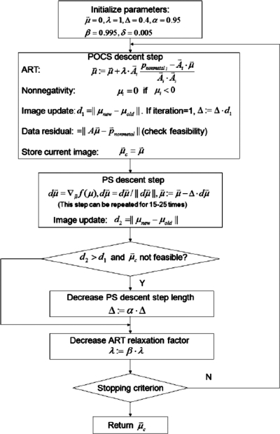
The implementation of the proposed algorithm involves selection of a set of parameters shown in Fig. 1. The optimization problem is specified by the metal excluded projection ${\stackrel{⃑}{p}}_{\text{nonmetal}}$ and the data-inconsistency parameter ε. The parameters that control the algorithm include the ART relaxation factor λ, initial step-length factor Δ, step lengths decreasing factors α and β, and the smoothing parameter δ in the PS function. The values shown in Fig. 1 are typical values used in generating the results in Sec. 3. The initial image was set to zero in this paper, but other choices are possible. The outermost loop in Fig. 1 contains two main components: Approaching data consistency through the POCS step and the PS steepest descent toward low PS images. The decreasing factors α and β is the key to control the respective step lengths for POCS and PS steepest descent. In the POCS step, the ART operator depends on the relaxation parameter λ, which starts at 1 and slowly decreases to 0 as the iteration progresses. The changes in the current image are computed after the POCS step and the PS descent step. The current image is stored in ${\stackrel{⃑}{\mu }}_c$ after each POCS step; once the optimality criterion is reached, it is the image stored in ${\stackrel{⃑}{\mu }}_c$ that is considered the “final” solution. The feasibility of the current image is checked after each POCS step by calculating the data residual $\Vert A\stackrel{⃑}{\mu }-{\stackrel{⃑}{p}}_{\text{nonmetal}}\Vert$. The initial PS descent step length is a fraction of a step length to an absolute image distance on the first iteration. In practice, it is effective when multiple small descent steps are taken for each large loop.¹⁹ The step-length adjustment is performed to have the image slide along the boundary of the feasible set by stopping reducing the PS descent step size once the data-tolerance condition is satisfied, while the ART relaxation factor is always decreasing. Thus the PS objective can have more power in moving the image toward a low PS one when the image is in the feasible pool. The optimization is terminated once the stopping criteria are met, i.e., the image estimate is feasible and k_d is below a certain value. The tolerance ε accommodates all sources of data inconsistency. For ideal simulations with no additive noise, zero data fidelity is approachable. However, lower data fidelity is at the cost of large number of iterations. The ideal ε should have a good trade-off between the size of the feasible set and the computation cost. To choose an appropriate ε, we simply run a number of iterations with POCS step alone and monitor the change of data fidelity. In the noiseless digital QA phantom case, for example, the data fidelity changes slowly after it falls below 2.5. Thus, the data tolerance for this reconstruction is set to ε=2.5, which is reached at iteration i=150. As the various parameters in the proposed algorithm are adjusted, the data fidelity converges to 2.5 and we choose the setting that yields the smallest k_d value. In the case of simulated noisy projection data or experimental data, zero data fidelity is generally not possible. When the value of ε is near ε_min, there is likely not much room in the set of feasible images. As a result, a larger data distance, which suggests an expanded feasible set of images, enables the PS objective to have a greater effect. Therefore, the data constraint is loosened by setting ε to a value that has a distance to ε_min. For example, the data tolerance ε is set to 41.8 for the digital QA phantom simulation with Poisson noise, although data fidelity is still slowly decreasing after it falls under this value. But how much we loosen from ε_min is heuristic rather than optimal. In general, we try to define a reasonably sized feasible set at a fair computational cost.

Figure 1.

Flowchart of the proposed constrained optimization approach (the parameters shown are used for the digital QA phantom).

With the current version of the proposed algorithm, there is no theoretical proof on the convergence properties and the image does not rigorously reach the solution of the optimization problem defined in Sec. 2B, but the reconstructed images showed that they are practically close to optimal.

Data acquisition

Two phantoms were used to evaluate the performance of the proposed constrained optimization algorithm. The first is a digital 2D QA phantom consisting of 350×350 (in pixels), 1×1 mm² per pixel. The outer circular background is composed of water, with tissue equivalent material in the inner circle. The two circles are with diameters 210 and 90 mm, respectively. The four objects within the inner circle are iron (left), brass (right), aluminum (upper), and bone (lower), of which the circles are with a diameter of 12 mm. Iron object has a slightly more complicated structure. The projection data are generated according to the fan-beam CT geometry. The distance of source-to-axis is 100 cm and source-to-detector distance of 150 cm. The projection data of each projection view consist of 500×1 pixels and the size of detector element is 1×1 mm². A total of 680 views projection data are simulated over 2π rotation. A monochromatic spectrum is assumed and the photon energy is set to 80 keV. Each projection value along a ray through the phantom is computed based on the known densities at 80 keV and intersection lengths of the ray with the pixels in the phantom. After the ideal or noise-free projection data $\stackrel{⃑}{p}$ is calculated, the noisy measurement I_i is generated according the following noise model:²¹

$$I_i=\text{Poisson}\left(I_0\text{\hspace{0.17em}exp}\left(-p_i\right)\right)+\text{Normal}\left(0,{\sigma }_e^2\right),$$ (14)

where I₀ is the incident x-ray intensity and ${\sigma }_e^2$ is the background electronic noise variance. In the simulation, I₀ is chosen as 2×10⁴ and ${\sigma }_e^2$ is chosen as 10. The noisy projection data can then be calculated as

$$p_i=\{\begin{array}{cc}\text{ln}\left(\frac{I_0}{I_i}\right)& I_i\ge T\\ \text{ln}\left(\frac{I_0}{T}\right)& I_i<T\end{array}\phantom{\}},$$ (15)

where T is a threshold to enforce that the logarithm transform is applied on positive numbers and it is chosen as 1 in this study.

The experimental study is done on a commercial calibration phantom (CatPhan^® 600 from the Phantom Laboratory, Inc., Salem, NY). In our experimental studies, the cone-beam CT projection data are acquired by using an Acuity simulator (Varian Medical Systems, Palo Alto, CA). The tube voltage is set to 125 kVp. The x-ray tube current was set at 10 mA and the duration of x-ray pulse at each projection view was 10 ms during the acquisition. The projection data were acquired in full-fan mode with the use of a full-fan bowtie filter. The source-to-axis distance is 100 cm and the source-to-detector distance of 150 cm. The number of projections for a full 360° rotation is 680. The dimension of each acquired projection image is 397 mm×298 mm, containing 1024×768 pixels. To save computational time during iterative reconstruction, the data at each projection view was down-sampled by a factor of 2 and only the central slice out of 768 projection data along the axial direction was chosen for reconstruction. The reconstructed image is 2D with size 350×350 pixels and the pixel size is 0.776×0.776 mm².

RESULTS

Digital QA phantom

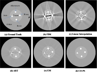
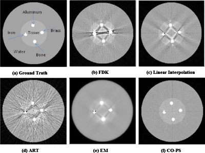
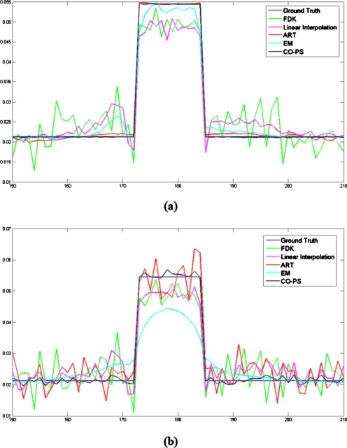
A 350×350 (in pixels) digital QA phantom is created to evaluate the proposed metal artifact reduction method. Figure 2 shows the reconstruction results using different approaches with noiseless projection data. FDK is applied to the original metal-contaminated projection data. Linear interpolation is applied to the original projection with the metal parts substituted by the linear interpolated data. ART, EM, and constrained optimization with penalized smoothness (CO-PS) are applied to the projection with the metal shadows removed. The ART and EM iteration procedures are terminated once the predefined data tolerance ε in the CO-PS method is attained. All the reconstructed images from the constrained optimization are fused with the binary metal image obtained from the procedure described in Sec. 2A by substituting the metal areas. Prominent artifacts are present in the FDK reconstruction. The linear interpolation method refers to that the missing projection data are first linearly interpolated based on neighboring values and then backprojected to the image domain. It partially suppressed the artifacts but has significant residuals remaining in the reconstruction. Two conventional iterative reconstruction algorithms, ART and EM, generally performed better in reducing the artifacts, but the residuals are still visible. The CO-PS removed the artifacts completely and produced the original phantom without blurring at the edge of the metal structures. Figure 3 shows the reconstruction results when Poisson noise is present in the projection data. It can be observed that FDK and ART have very noisy reconstructions with severe streaking artifacts present. EM suppressed artifacts and noise at the same time but at the cost of an oversmoothed image. Linear interpolation method can partially reduce the artifacts but does not seem to suppress noise effectively. CO-PS not only removed metal artifacts completely, but also had a significantly reduced noise level of the reconstructed image. Compared to other methods, CO-PS had a superior performance in suppressing metal artifacts and noise at the same time. The transverse image profiles through row 203 shown in Fig. 4 also agree with the reconstructions in Fig. 23. In the noiseless case, the CO-PS profile (black line) almost superimposes the ground truth (blue line). In the noisy case, the CO-PS profile is still very close to the noise-free ground truth, with only small variations that indicate the presence of noise.

Figure 2.

Reconstructed images of the digital QA phantom with noiseless projection data: (a) Ideal phantom, (b) analytical FDK reconstruction, (c) reconstruction from linear interpolated projection data, (d) ART reconstruction, (e) EM reconstruction, and (f) CO-PS reconstruction with ε=2.5, k_d=0.250. All reconstructions are shown with metal objects combined.

Figure 3.

Reconstructed images of the digital QA phantom with simulated Poisson noise on the projection data. The simulated incident photon number isN₀=2×10⁴. (a) Ideal phantom, (b) analytical FDK reconstruction, (c) reconstruction from linear interpolated projection data, (d) ART reconstruction, (e) EM reconstruction, and (f) CO-PS reconstruction with ε=41.8, k_d=2.54. All reconstructions are shown with metal objects combined.

Figure 4.

Transversal profile through row 203 of the reconstructed images shown in Figs. 23. (a) Noiseless case and (b) noisy case.

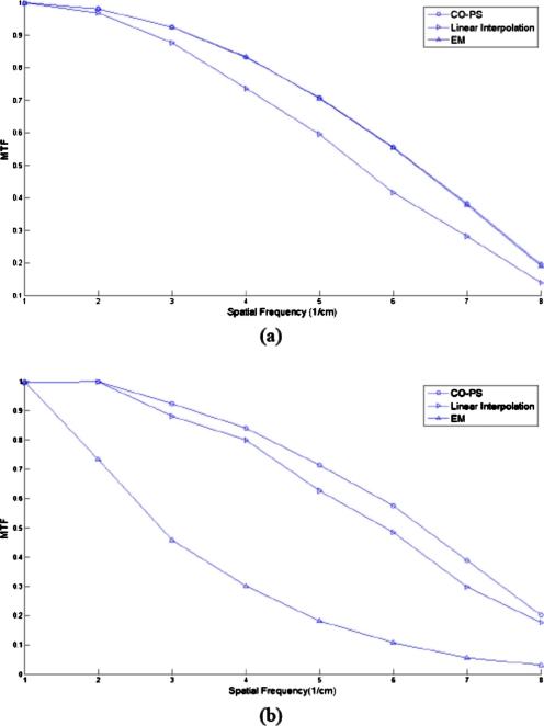
The modulation transfer function (MTF) that characterizes the spatial resolution of images is calculated to show further comparisons of different approaches. The dashed line segment indicated in Fig. 2a provides a step function and the MTF can be obtained by calculating one-dimensional Fourier transform. The MTF curves of CO-PS are shown in Fig. 5 with comparison to the MTF curves of EM and linear interpolation, which have relatively better reconstructions in Figs. 23. It can be observed that CO-PS produces better image resolution.

Figure 5.

MTF curves of different image reconstruction algorithms. (a) Noiseless case and (b) noisy case.

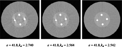
Figure 6 shows the CO-PS reconstructions with the same data tolerance ε and different k_d values when Poisson noise is present. As k_d decreases, the reconstructed image is visibly improved in terms of both artifacts suppression and noise performance.

Figure 6.

CO-PS reconstructions with the same data tolerance and different k_d values. Images are reconstructed from Poisson noise corrupted projection data with incident photons N₀=2×10⁴. All reconstructions are shown with metal objects combined.

CatPhan^® 600 Phantom

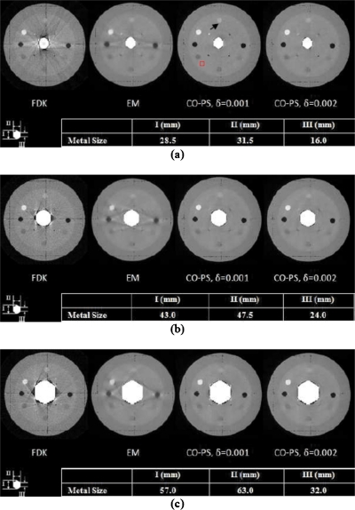
An experimental study was conducted using the CatPhan^® 600 phantom with a hexagonally shaped metal object embedded in the central region. The projection data were acquired using low-dose protocol (10 mA∕10 ms). Figure 7 shows CO-PS reconstructions together with FDK calculations for three differently sized metal objects. All the images shown are fused with the binary metal images. Extensive streak artifacts are present in the FDK results. The EM method, similar to the digital phantom case, partially suppressed the artifacts but the image contrast seemed to be compromised. In comparison, CO-PS almost completely suppressed the metal artifacts with the image contrast retained and edge structures well preserved. In Fig. 7, the CO-PS reconstructions are shown with two smoothing parameters δ=0.001 and δ=0.002. As δ increases, the CO-PS reconstruction slight loses contrast but is visibly smoother.

Figure 7.

Reconstructed images of CatPhan^® 600 phantom with different metal object sizes. Two different smoothing parameters are applied to CO-PS reconstructions. All reconstructions are shown with metal objects combined.

In the CatPhan^® 600, there are several circles of different intensities which can be used to quantify the contrast-to-noise (CNR) of the reconstructed images. The circle indicated by the black arrow in Fig. 7 is selected as the region of interest (ROI) for the calculation of the CNR in the image reconstructed by different algorithms. The contrast was calculated as the absolute difference between the mean value of the region inside the ROI and the mean value of the uniform background region. The noise level was characterized by the standard deviation of a uniform area of size 10×10 pixels indicated by the red square. The CNR was defined as the contrast divided by the standard deviation. Table 1 lists the CNRs of FDK, EM, and CO-PS with two different δ values. It can be observed that the CNR of CO-PS reconstruction is comparable to that of EM and significantly higher than that of the FDK reconstructed image. As δ doubles, the CNR of CO-PS reconstruction increases accordingly. It indicates that although the contrast is slightly compromised with larger δ value, the noise is better suppressed. Also, the parameter δ gives us extra flexibility in selecting the reconstructed image we need.

Table 1.

CNRs of the indicated ROI in Fig. 7.

	FDK	EM	CO-PS, δ=0.001	CO-PS, δ=0.002
Metal size 1	1.484	6.010	6.097	6.266
Metal size 2	1.664	5.685	4.378	6.381
Metal size 3	1.991	4.440	3.459	4.574

DISCUSSION

A constrained optimization algorithm for metal artifacts removal and noise suppression has been described. In the proposed algorithm, the metal-shadow-corrupted projections are treated as a system with missing data and a constrained optimization model is then utilized to select an optimal solution out of a feasible set. A novel penalized smoothness function with an edge-preserving prior is introduced to encourage smooth and edge-preserved image solution. Simulation and experimental results show that, in general, the proposed algorithm can significantly improve the widely used FBP-type methods as well as the basic iterative methods.

The PS objective is designed to select images that are piecewise smooth and can faithfully reconstruct the image when the assumption is valid. Similarly, TV objective can be chosen when images are with sparse GMIs. However, the TV objective is not expected to have a particular effect in suppressing noise. PS objective seems to be a suitable choice if both artifacts removal and noise suppression are pursued. A careful control of the smoothing parameters is recommended in this case to avoid oversmoothed solutions.

A possible limitation of the constrained optimization approach is that the iterative algorithms are usually very sensitive to system configurations and the quality of projection data. For computer simulations in which every condition is accurately set, the constrained optimization works very well and the quality of reconstructed images is a monotonic function of the number of iterations. However, our study using experimental data shows that the performance of constrained optimization degrades when system geometry mismatch exists, which sets a higher standard on experimental setup and data acquisition. This also leaves a problem of parameter setting in solving the constrained optimization. In this work, the parameters, including the initial ART relaxation factor, initial gradient descent step length, and decreasing factors, are empirically determined, which may not guarantee the best performance of the algorithms. For experimental studies, manual adjustment of the parameters may be needed to accommodate different data qualities and ensure good performance of the algorithm for different cases. Further work is useful to automatically determine the optimal parameters for a given set of experimental data by using some random sampling procedures.

The computation efficiency is not yet a particular concern in our work. To reconstruct a 350×350 (in pixels) image, the constrained optimization algorithm took about 45 s to finish one loop on a 2.4 GHz PC with 2G RAM. There are several ways to improve computational efficiency. One way to optimize the problem solving procedure, for example, is to void the gradient descent when POCS has not yet started to drag the image close to the feasible set. Graphics processing unit acceleration can also be used to save time on the vector computations.

In conclusion, the constrained optimization algorithms have been developed for metal artifacts removal. Superior performance of the algorithms has been demonstrated using both simulation and experimental data. Overall, images with much reduced artifacts can be obtained using the proposed approaches. Finally, these algorithms do not discriminate the source of missing data in the raw projections. They can thus be easily generalized to deal with other incomplete data problems with various x-ray scanning geometries and trajectories.

References

- Mahnken A. H., Raupach R., Wildberger J. E., Jung B., Heussen N., Flohr T. G., Günther R. W., and Schaller S., “A new algorithm for metal artifact reduction in computed tomography,” Invest. Radiol. 38, 769–775 (2003). 10.1097/01.rli.0000086495.96457.54 [DOI] [PubMed] [Google Scholar]
- Srinivasa N., Ramakrishnan K. R., and Rajgopal K., “Image reconstruction from incomplete projection,” J Med Life Sci Eng 14, 1–19 (1997). [Google Scholar]
- Zhao S., Robertson D. D., and Wang G., “X-ray CT metal artifact reduction using wavelets: An application for imaging total hip prostheses,” IEEE Trans. Med. Imaging 19, 1238–1247 (2000). 10.1109/42.897816 [DOI] [PubMed] [Google Scholar]
- Wang G. et al. , “Iterative deblurring for CT metal artifact reduction,” IEEE Trans. Med. Imaging 15, 657–664 (1996). 10.1109/42.538943 [DOI] [PubMed] [Google Scholar]
- Robertson D. D. et al. , “Total hip prosthesis metal-artifact suppression using iterative deblurring reconstruction,” J. Comput. Assist. Tomogr. 21, 293–298 (1997). 10.1097/00004728-199703000-00024 [DOI] [PubMed] [Google Scholar]
- Nuyts J., De Man B., and Dupont P., “Iterative reconstruction for helical CT: A simulation study,” Phys. Med. Biol. 43, 729–737 (1998). 10.1088/0031-9155/43/4/003 [DOI] [PubMed] [Google Scholar]
- Williamson J. F., Whiting B. R., Benac J., Murphy R. J., Blaine G. J., O’Sullivan J. A., Politte D. G., and Snyder D. L., “Prospects for quantitative computed tomography imaging in the presence of foreign metal bodies using statistical image reconstruction,” Med. Phys. 29, 2404–2418 (2002). 10.1118/1.1509443 [DOI] [PubMed] [Google Scholar]
- Ebraheim N. A. et al. , “Reduction of postoperative CT artefacts of pelvic fractures by use of titanium implants,” Orthopedics 13, 1357–1358 (1990). [DOI] [PubMed] [Google Scholar]
- Ling C. C. et al. , “CT-assisted assessment of bladder and rectum dose in gynecological implants,” Int. J. Radiat. Oncol., Biol., Phys. 13, 1577–1582 (1987). 10.1016/0360-3016(87)90327-0 [DOI] [PubMed] [Google Scholar]
- Wang G. et al. , “Iterative x-ray cone-beam tomography for metal artifact reduction and local region reconstruction,” Microsc. Microanal. 5, 58–65 (1999). 10.1017/S1431927699000057 [DOI] [PubMed] [Google Scholar]
- Toft P., “A very fast implementation of 2D iterative reconstruction algorithms,” IEEE Proc Med Imaging Conf 3, 1742–1746 (1996). [Google Scholar]
- Kalender W. A., Hebel R., and Ebersberger J. A., “Reduction of CT artifacts caused by metallic implants,” Radiology 164, 576–577 (1987). [DOI] [PubMed] [Google Scholar]
- Klotz E., Kalender W. A., Sokiranski R., and Felsenberg D., “Algorithms for reduction of CT artifacts caused by metallic implants,” SPIE Med Imaging IV 1234, 642–650 (1990). [Google Scholar]
- Lewitt R. M. and Bates R. H. T., “Image reconstruction from projections: III. Projection completion methods,” Optik (Stuttgart) 50, 189–204 (1978). [Google Scholar]
- Feigenberg S. J., Paskalev K., McNeeley S., Horwitz E. M., Konski A., Wang L., Ma C., and Pollack A., “Comparing computed tomography localization with daily ultrasound during image-guided radiation therapy for the treatment of prostate cancer: A prospective evaluation,” J. Appl. Clin. Med. Phys. 8, 2268–2268 (2007). 10.1120/jacmp.v8i3.2268 [DOI] [PMC free article] [PubMed] [Google Scholar]
- Wang J., Li T., and Xing L., “Iterative image reconstruction for CBCT using edge-preserving prior,” Med. Phys. 36, 252–260 (2009). 10.1118/1.3036112 [DOI] [PMC free article] [PubMed] [Google Scholar]
- Wang J. and Xing L., “Accurate determination of the shape and location of metal objects in x-ray computed tomography,” Proc. SPIE 7622, 76225A–76225A-10 (2010). [DOI] [PMC free article] [PubMed] [Google Scholar]
- Meng B., Wang J., and Xing L., “Sinogram processing and binary reconstruction for determination of the shape and location of metal objects in computed tomography (CT),” Med. Phys. 37, 5867–5875 (2010). 10.1118/1.3505294 [DOI] [PMC free article] [PubMed] [Google Scholar]
- Sidky E. Y. and Pan X., “Image reconstruction in circular cone-beam computed tomography by constrained, total-variation minimization,” Phys. Med. Biol. 53, 4777–4807 (2008). 10.1088/0031-9155/53/17/021 [DOI] [PMC free article] [PubMed] [Google Scholar]
- Fessler J. A., “Penalized weighted least-squares image-reconstruction for positron emission tomography,” IEEE Trans. Med. Imaging 13, 290–300 (1994). 10.1109/42.293921 [DOI] [PubMed] [Google Scholar]
- Wang J., Li T., Lu H. B., and Liang Z. R., “Penalized weighted least-squares approach to sinogram noise reduction and image reconstruction for low-dose x-ray computed tomography,” IEEE Trans. Med. Imaging 25, 1272–1283 (2006). 10.1109/TMI.2006.882141 [DOI] [PMC free article] [PubMed] [Google Scholar]
- Li T. F., Li X., Wang J., Wen J. H., Lu H. B., Hsieh J., and Liang Z. R., “Nonlinear sinogram smoothing for low-dose x-ray CT,” IEEE Trans. Nucl. Sci. 51, 2505–2513 (2004). 10.1109/TNS.2004.834824 [DOI] [Google Scholar]
- Wang J., Lu H., Liang Z., Eremina D., Zhang G., Wang S., Chen J., and Manzione J., “An experimental study on the noise properties of x-ray CT sinogram data in Radon space,” Phys. Med. Biol. 53, 3327–3341 (2008). 10.1088/0031-9155/53/12/018 [DOI] [PMC free article] [PubMed] [Google Scholar]
- Sauer K. and Bouman C., “A local update strategy for iterative reconstruction from projections,” IEEE Trans. Signal Process. 41, 534–548 (1993). 10.1109/78.193196 [DOI] [Google Scholar]
- Sukovic P. and Clinthorne N. H., “Penalized weighted least-squares image reconstruction for dual energy x-ray transmission tomography,” IEEE Trans. Med. Imaging 19, 1075–1081 (2000). 10.1109/42.896783 [DOI] [PubMed] [Google Scholar]
- La Riviere P. J., Brian J. G., and Vargas P. A., “Penalized-likelihood sinogram restoration for computed tomography,” IEEE Trans. Med. Imaging 25, 1022–1036 (2006). 10.1109/TMI.2006.875429 [DOI] [PubMed] [Google Scholar]
- Perona P. and Malik J., “Scale-space and edge-detection using anisotropic diffusion,” IEEE Trans. Pattern Anal. Mach. Intell. 12, 629–639 (1990). 10.1109/34.56205 [DOI] [Google Scholar]
- Candes E., Romberg J., and Tao T., “Robust uncertainty principles: Exact signal reconstruction from highly incomplete frequency information,” IEEE Trans. Inf. Theory 52, 489–509 (2006). 10.1109/TIT.2005.862083 [DOI] [Google Scholar]
- Candès E., Romberg J., and Tao T., “Stable signal recovery from incomplete and inaccurate measurements,” Commun. Pure Appl. Math. 59, 1207–1223 (2006). 10.1002/cpa.20124 [DOI] [Google Scholar]
- Boyd S. and Vanderberghe L., Convex Optimization (Cambridge University Press, Cambridge, 2004). [Google Scholar]