

Abstract
The role of modelling and simulation on the systemic analysis of living systems is now clearly established. Emerging disciplines, such as Systems Biology, and world-wide research actions, such as the Physiome project or the Virtual Physiological Human, are based on an intensive use of modelling and simulation methodologies and tools. One of the key aspects in this context is to perform an efficient integration of various models representing different biological or physiological functions, at different resolutions, spanning through different scales. This paper presents a multi-formalism modelling and simulation environment (M2SL) that has been conceived to ease model integration. A given model is represented as a set of coupled and atomic model components that may be based on different mathematical formalisms with heterogeneous structural and dynamical properties. A co-simulation approach is used to solve these hybrid systems. The pioneering model of the overall regulation of the cardiovascular system, proposed by Guyton, Coleman & Granger in 1972 has been implemented under M2SL and a pulsatile ventricular model, based on a time-varying elastance has been integrated, in a multi-resolution approach. Simulations reproducing physiological conditions and using different coupling methods show the benefits of the proposed environment.
Keywords: Cardiovascular System; Computer Simulation; Humans; Models, Cardiovascular; Systems Biology
Keywords: Multiformalism modelling, Multiresolution, Simulation, Integrative physiology
1. Introduction
Modelling and simulation have proven particularly useful for the analysis of complex living systems. A variety of models have been proposed for different biological or physiological functions, at different resolutions. These models can be classified according to their level of i) structural integration, ii) functional integration and iii) data integration, as proposed by McCulloch and Huber (2002), and they can be projected into a three-dimensional space defined by these axes.
The structural integration (vertical axis) spans from the sub-cellular level to the whole body and the population level, covering different spatio-temporal scales. The integration of different biological or physiological functions (e.g. cardiac electrical activity, cardiac mechanical activity, body fluid regulation, autonomic regulation, etc…) is represented in the horizontal axis. Finally, the third axis concerns the level of knowledge represented in the model: one end of this axis corresponds to black-box models, which are limited to the reproduction of observations, and the other end corresponds to models integrating the most detailed biochemical, physical or physiological knowledge available.
Most of the models proposed in the literature can be associated with a single 3D ’cell’ of this space, as they are usually developed to reproduce a specific function, at a given scale and level of knowledge integration, adapted to the problem under consideration. A major goal of current efforts in the emerging fields of systems biology and integrative physiology is to ease the integration of models proposed by different authors, for different functions (horizontal integration), different scales (vertical integration) and different levels of data/knowledge representation, in order to analyse the complex interactions governing biological systems. International actions such as the Physiome project (Hunter, 2004) and the Virtual Physiological Human (VPH) (Fenner et al., 2008) are headed in this direction.
An interesting example of horizontal integration is the pioneering work of Guyton, Coleman and Granger (1972) on the analysis of the overall regulation of the cardiovascular system. They proposed an integrated mathematical model, composed of a set of ’blocks’ representing the most relevant physiological sub-systems involved in cardiovascular regulation. Simulation results obtained from this model have been used to perform a simultaneous analysis of the main effects triggered by specific circulatory stresses and even to predict behaviours that were only observed experimentally later on (Guyton and Hall, 1995). It was also used to identify in which parts of the system new knowledge was required, helping to propose new experimental investigations. However, this model only represents a basic description of the cardiovascular regulatory system and the resolution of each one of the constituting blocks was not sufficient to represent most interesting pathologies.
Models including vertical integration have also been proposed in the literature, in particular in the field of cardiology. For example, cell-to-organ representations of the electrical activity of the heart have been proposed by different authors (Fenton et al., 2005; Nickerson et al., 2006; Noble, 2004). Certain works include, to some extent, both vertical and horizontal integration, such as the electromechanic models of the cardiac activity (Dou et al., 2009; Kerckhoffs et al., 2007; Usyk and McCulloch, 2003; Watanabe et al., 2004). These models have proven useful in a number of situations; however, their complexity and their significant computational costs make it difficult to perform essential tasks such as sensitivity analysis and parameter identification. Moreover, the absence of a coupling with other physiological systems may limit the definition of appropriate boundary conditions.
It is impossible to realize a complete horizontal and vertical integration at the highest structural resolution, as this would demand unlimited resources. A way to get round this problem can be to represent different functions at different scales, in a multi-resolution approach (Bassingthwaighte et al., 2006). However, this is a challenging task. Models in different sub-spaces of the above-mentioned 3D space are often represented using different mathematical formalisms, which can be continuous (such as ordinary, stochastic, delay or partial differential equations) or discrete (cellular automata, agent-based models, etc.), to name a few. Coupling these different models in a multi-formalism approach is not simple. Moreover, the correspondence of detailed and simplified models, via homogenisation methods for example, can be difficult to obtain and may require specific modelling and simulation environments.
A number of commercial or academic, open-source environments for modelling and simulation are available today, either for generic applications, such as Mathematica, MATLAB/Simulink, COMSOL, Modellica/OpenModellica, or specific to the field of systems biology and integrative physiology, such as e-Cell (Tomita, 2001), VirtualCell (Loew and Schaff, 2001) or JSim (Raymond et al., 2003), at the cellular and subcellular levels, or CMISS (Blackett et al., 2005) and Continuity† for cell to organ integration. These modelling environments integrate, to different extents, the set of requirements identified, for example, in the context of the VPH, for the definition of a common set of tools allowing model integration (Fenner et al., 2008). In particular, most of the specific environments are compatible with standard model representation schemes, such as SBML or CellML. However, the coupling of heterogeneous models (with different formalisms, temporal dynamics, etc.) cannot be efficiently handled with current tools and new propositions are emerging in this sense (Hetherington et al., 2007).
This work presents the current status of a multi-formalism modelling and simulation library (M2SL) that is in active development in our laboratory, which may ease model integration in this context. The library was designed around the following requirements: i) it should be based on a compiled language and a distributed, object-oriented approach; ii) the library must be capable of coupling models developed under different mathematical formalisms; iii) efficient schemes for the simulation of coupled model components, presenting heterogeneous time-scales should be integrated within the library; iv) the definition of a specific simulator for each model component should be possible and v) an API for sensitivity analysis and parameter identification should be provided.
The first section of this paper presents a general description of M2SL and the underlying methods integrated in the library. Example applications are proposed in §3, using the Guyton 1972 model as an illustration. The last section recalls the main properties of the library and depicts current developments.
2. General description of the M2SL library
M2SL is a collection of generic C++ classes that has been developed for modelling and simulating complex systems using a combination of different modelling formalisms. Two main approaches have been identified for modelling and simulating these multiformalism systems (Lara and Vangheluwe, 2002; Vangheluwe et al., 2002):
Formalism-transformation: All the components of a system are transformed into a single formalism, for which a simulator is available. This approach has been mainly developed by Zeigler by coupling the Discrete EVent System Specification (DEVS) and the Differential Equation System Specification (DESS) formalisms (Zeigler et al., 2000), with DEVS&DESS-based tools. Other solution methods using DEVS as a common formalism, such as the Quantized State Systems (QSS) Kofman (2004) have been proposed.
Co-Simulation: Each component of the system is processed by a formalism-specific simulator, in a distributed scheme, and perform inter-component coupling at the input/output trajectory level.
The co-simulation approach was chosen for our work, as it avoids the limits and the time-consuming processes associated with the formalism-transformation approach and maintains the possibility of using model-specific simulators that are common in complex physiological models.
A global model is defined in M2SL by coupling a set of components, made up of a combination of two types of model objects: atomic models (Ma) and coupled models (Mc). Atomic models represent a specific component of the system under study, using a given formalism (for example, a continuous model of a single myocite). Coupled models are composed of a hierarchy of interconnected coupled or atomic sub-models, that may be defined with different formalisms, as represented in figure 1 (for example, a tissue-level model composed of a set of coupled myocite atomic models (Defontaine et al., 2005)).
Figure 1.
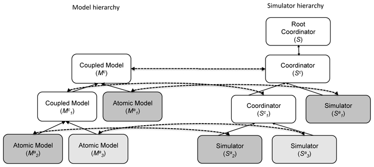
On the left side: Functional diagram representing the hierarchy of a coupled model Mc, composed of a set of atomic and coupled sub-models (solid arrows represent the relation ’is a component of’). On the right side: Dynamically-created simulator hierarchy, defined at runtime by the Root Coordinator (S). Each model is associated with the corresponding atomic simulator or coordinator (dotted arows). Grey-levels represent different mathematical formalisms used to define each model and its corresponding simulator.
At run-time, a global simulator S, called the ’Root coordinator’ is created. It will follow the global model hierarchy to define a parallel simulator hierarchy, in which a specific atomic simulator will be associated with each atomic model . A continuous atomic model will be associated with a continuous simulator, and a discrete atomic model will be associated with a discrete simulator. These simulators will adapt their properties (such as the integration step size, in the continuous case) according to the dynamics of the corresponding atomic model. Coupled models are associated with a particular kind of simulator called ’coordinators’ (Sc), that will mainly handle the input-output relations and time synchronisation between the constituting sub-models. These two points represent the main difficulty for the development of a multi-formalism environment based on the co-simulation approach.
(a). Input-output coupling and temporal synchronisation
The problems of input-output coupling and temporal synchronisation may be stated as follows: Let an atomic model Ma and a coupled model Mc be defined as:
| (2.1) |
| (2.2) |
where F is the description formalism, I is a vector of one or more inputs, E is the vector of state variables, P are the model parameters and {Mi} is the set of n atomic or coupled model objects constituting coupled model Mc.
As previously mentioned, the co-simulation approach that we have retained is based on a parallel between a model Mk and its corresponding simulator Sk, according to their kind (k = {a, c} for atomic or coupled, respectively) and their description formalism F. These simulators can be represented as:
| (2.3) |
where Ps are the simulation parameters and O is the output of the model, obtained from a given simulation.
The coupling of two atomic models and , defined respectively by formalisms F2 and F3, in which the outputs of are used as inputs to is performed within a coupled model object, . From the simulators standpoint, this coupling can be stated as follows:
| (2.4) |
| (2.5) |
| (2.6) |
where T is a transformation permitting to solve the input-output coupling in equation 2.5. One of the most important aspects of co-simulation is thus to define an appropriate transformation T, which will be applied at the coordinator level, at each coupling time-step. A definition of such a transformation and the handling of the temporal synchronisation between coordinators and atomic simulators are presented in the following sections.
(i). Input-output coupling
Input-output coupling is performed via specific interface objects. Depending on the formalisms involved, this coupling can be done by means of sampling-and-hold, filtering and interpolation (linear, splines, etc.), or quantisation methods. Experience shows that the definition of input-output coupling of two models represented by different formalisms is problem-specific and depends on the kind of formalisms involved (discrete, continuous or event-based). For instance, in the previous example of equation 2.5, if O3 is discrete while expects continuous inputs, a sample-and-hold method can be used between two consecutive coupling steps. Linear or higher-order interpolation can also be applied. If O3 is continuous while I2 expects discrete values, quantisation methods can be used. Interface objects for input-output coupling can also be useful when associating two models using the same formalism, but using different temporal or spatial resolutions. An example of this latter point will be presented in §3 c.
(ii). Temporal synchronisation
The problem of temporal synchronisation in a co-simulation approach resides on the fact that each atomic model is processed by a particular simulator, which may have specific simulation parameter values. A temporal synchronisation strategy is thus needed to synchronize these simulators (and coordinators), perform input-output coupling and obtain the global simulation output values.
Consider the coupled model depicted in figure 2, in which all atomic models ( , i = 2, … n) are represented in a continuous formalism and a hierarchy of continuous atomic simulators ( , i = 2, … n), each one with its own fixed or adaptive integration step-size (δta,i), has been defined. The input-output coupling of atomic models ( ) is performed by and at fixed or adaptive intervals, denoted δtc, in which a temporal synchronisation of all atomic models occur, and outputs of the coordinator are calculated.
Figure 2.

Functional diagram of an example coupled model composed of n atomic models and its corresponding simulator hierarchy.
At the current state of development, three different schemes for synchronising δta,i and δtc, noted ST1−ST3, have been proposed and implemented in the library (figure 3):
Figure 3.

Graphical representation of the time synchronization schemes implemented in the library, based on the example of coupled models on figure 2. a) Fixed-step method; b) Adaptive synchronisation and simulation, with the smallest atomic timestep and c) Synchronisation at a fixed time-step (δtc) and atomic simulation with independent, adaptive time-steps δta;i.
ST1: Simulation and synchronisation with a unique, fixed time-step (figure 3-a). In this approach, the simulation step is δta,i = δtc for all the elements, regardless of their local dynamics. This is the simplest way, which is indeed the same used in centralized simulators that update all the state-variables of the model in a single simulation loop. This approach does not handle efficiently the heterogeneity of the local dynamics associated with each component of the model.
ST2: Adaptive atomic simulation and synchronisation at the smallest time step required by any of the atomic models (figure 3-b). The simulation time-step for each atomic model, δta,i(t) and the coupling time-step δtc(t) are adaptive, and are updated after each coupling step with δtc(t) = mini [δta,i(t)] and δta,i(t) = δtc(t), ∀i. This scheme is a completely adaptive approach, requiring minimum user interaction. However, the benefits of this method are only observed when the dynamics of atomic simulators are similar and these dynamics present significant differences through time.
ST3: Synchronisation at a fixed time-step and atomic simulation with independent, adaptive time-steps (figure 3-c). Here, each atomic simulator evolves with its own adaptive simulation step δta,i(t) and all simulators are coupled at fixed intervals δtc. The objective is to exploit the different dynamics of the atomic models in order to reduce simulation time. For instance, if model shows slower dynamics than model , δta,2 will be greater than δta,3. This approach benefits from the heterogeneity of the dynamics in each atomic simulator, but the value of δtc should be chosen carefully, with δtc(t) ≥ maxi [δta,i(t)].
Classical algorithms for the adaptation of the simulation time-step can be used with methods ST2 and ST3. It should be noticed that, in a typical centralized method, equivalent strategies for ST1 and ST2 can be applied. However, implementation of ST3 is only possible using a distributed co-simulation architecture.
(b). Implementation aspects
M2SL is composed of two main abstract classes, ’Model’ and ’Simulator’, based on the definitions in equations (2.1) and (2.3), and a set of derived classes. The ’Model’ class implements properties and operators that are common to all model components. The main properties include: i) vector objects representing state variables, inputs, outputs and model parameters; ii) a specific structure to represent the formalism in which a given model is defined; iii) structures defining the preferred simulator and simulation parameters; iv) a pointer to the corresponding simulator object; v) a vector of ’Model’ objects (called ’components’) which contains the sub-models associated with a coupled model.
The ’components’ vector also allows for the differentiation between atomic or coupled models: if this vector contains no elements in an object derived from this class, it is considered as an atomic model, otherwise, it will be treated as a coupled model. The ’Model’ class also includes operators to: i) create an instance of the model, allocate storage space and create model components (constructor method); ii) initialize state variables; iii) setup internal properties before starting a simulation; iv) update state variables, read inputs, and solve algebraic equations and constraints; v) estimate the appropriate simulation time-step; vi) calculate derivatives (in the case of differential models); vii) calculate model outputs; viii) setup internal properties after the end of a simulation. In the abstract ’Model’ class, these operators are either empty or containing the common functions for all model types. Creating a model under M2SL thus implies creating one class for each model component (each class inheriting directly or indirectly from the Model class), that will integrate specific functions into these generic operators (method overriding).
The ’Simulator’ abstract class implements properties and operators concerning generic simulation tasks. Properties include: a pointer to the corresponding model object; a structure with the simulation parameters, corresponding to Ps in equation (2.3), a structure storing the formalisms supported by the simulator, the current simulation time, etc. This class includes operators to initialize, start or finish a simulation. It also defines abstract operators to update state variables, calculate outputs and estimate the next simulation time-step. These operators are overridden by each descendant of the ’Simulator’ class and are directly linked to the corresponding operators on the ’Model’ class.
Two particular classes are derived from the ’Simulator’ class: the ’RootCoordinator’ and the ’Coordinator’. As previously described, the ’RootCoordinator’ will follow the model hierarchy, create the simulator hierarchy associating each model with an appropriate simulator, initialize simulator and model objects and perform the global simulation loop. The ’Coordinator’ class applies similar tasks for coupled models. The simulation loops on these two classes will recursively apply each one of the following steps: i) estimate the next δta,i and its δtc, according to the selected temporal synchronisation strategy, ii) update state variables, iii) calculate derivatives (for continuous atomic simulators), iv) calculate outputs and v) perform input-output coupling. Each one of these steps is applied for each simulator object in the hierarchy (and, thus, to their corresponding model objects), before proceeding to the next step.
Concerning atomic simulators, a set of classes has been developed for discrete and continuous simulators. Continuous simulators are based on the numerical functions of the GNU Scientic Library (GSL) and include all the integration methods and all the algorithms to adapt the integration step-size available in the GSL. Adding new simulators, adapted to different formalisms, for example, can be easily done by overriding the appropriate operators from the Simulator class.
A typical simulation session is thus performed by implementing the following steps:
Create an instance of the global model, which will recursively create instances for all its components.
Define the Root Coordinator simulation parameters, including the temporal synchronisation scheme and the total simulation time for this session.
Create an instance of the Root Coordinator class, specifying the simulation parameter structure.
Associate the model object with the Root Coordinator object. This will create the whole simulation hierarchy, as shown in figure 1.
Send a ’Simulate’ message to the Root Coordinator, which will apply the global simulation loop.
3. Results and discussion
This section presents a modular implementation of the Guyton 1972 model (G72), based on M2SL. This legacy model has been chosen as an example, as its implementation presents the typical difficulties encountered when trying to perform horizontal and vertical model integration. In particular, the problem of an efficient handling of the heterogeneous temporal scales of the model components, which was already mentioned by the authors in their original paper (Guyton et al., 1972), is handled in this section. For instance, in the G72 model, long-term regulatory effects of the cardiovascular activity (such as the renin-angiotensin-aldosterone system) present time constants measured in hours or days, while the short-term regulation (mainly by the baroreflex) presents time constants of the order of the second. A detailed presentation of this model can be found elsewhere (Thomas et al., 2008). Section 3 b presents simulation results with the different strategies of temporal synchronisation integrated in M2SL.
Another reason for choosing this model is that we consider it as a good starting point for the development of a ’core-modelling environment’ that could be useful in the framework of the VPH, for coupling multi-resolution model components. This is one of the main objectives of the SAPHIR project (Thomas et al., 2008). Section 3 c shows an example of multi-resolution integration in which the non-pulsatile ventricles of the original G72 model are substituted with pulsatile, elastance-based models.
(a). Implementation of the G72 model under M2SL
In order to implement the G72 model using M2SL, atomic model classes were created for each one of the ’blocks’ described on the original paper. Additionally, one coupled model class (the ”Guyton72” class) was defined, to create instances of all other classes, as sub-model components, and to perform input-output couplings between these components. All these classes inherit from the abstract ’Model’ class. A class diagram of the implementation is presented in figure 4. Two continuous formalisms are used in the description of this model: ordinary differential equations (ODE) and algebraic equations (AE). The preferred continuous simulator defined for the 18 atomic models with F = ODE, is the fourth-order Runge-Kutta method.
Figure 4.
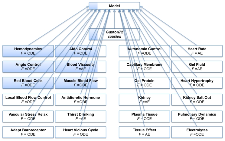
Simplified class diagram of the M2SL implementation for the G72 model. The class ’Guyton72’ is the coupled model that links all other atomic models as components. The description formalism F of each component is also displayed: algebraic equations (AE) and ordinary differential equations (ODE).
Verification of our M2SL implementation of the model was carried out by repeating the simulated experiments, published in the 1972 Guyton et al. paper, and comparing the simulated results with the output from the original FORTRAN program. We obtained this reference output data from Ron J. White, who worked in Guyton’s laboratory at the time.
The first experiment, which will be called benchmark 1 (BM1), is the simulation of sudden severe muscle exercise during 9 minutes. After 30 seconds, the exercise parameter (EXC) was modified to 60 times its normal value, corresponding to a whole body metabolism increase of approximately 15 times and the time constant for the local vascular response to metabolic activity (A4K) was reduced by 40. After 2 minutes, EXC was set to its normal value. At the beginning of exercise, cardiac output and muscle blood flow rose immediately. Urinary output fell to its minimum level while arterial pressure increased moderately. Muscle cell and venous PO2 decreased rapidly. Muscle metabolic activity instantaneously increased before falling considerably because of the development of a metabolic deficit in the muscles. After completing exercise, muscle metabolic activity decreased to below normal, but cardiac output, muscle blood flow, and arterial pressure remained elevated for a while as the oxygen activity returned to normal.
The second experiment (BM2) is the simulation of an atrioventricular fistula during 9 days. After 2 hours, the fistula parameter (FIS) was set to a value equal to −0.05, which would double cardiac output; then, after 4 days, the fistula is closed (FIS = 0). The fistula caused an instantaneous effect on cardiac output, total peripheral resistance and heart rate. Concurrently, urinary output falls to its minimum. To compensate the fistula, extracellular fluid volume and blood volume increased. As a consequence, arterial pressure, heart rate, and urinary output reached normal values after few days, while peripheral resistance and cardiac output doubled. The closing of the fistula also caused dramatic effects: the cardiac output instantaneously fell and the peripheral resistance rapidly increased. The rapid increase in urinary output makes the extracellular fluid volume and the blood volume decrease to normal values. After several days, all physiological variables present almost normal values. Figures 5 and 6 show the close match between M2SL simulations and the results from the original Guyton model.
Figure 5.

Comparison of M2SL simulations (black curves) with the original Guyton model (dotted curves) during BM1 (sudden severe muscle exercise). Total experiment time was 9 min. VUD (urinary output in ml/min), PVO (muscle venous oxygen pressure in mm Hg), PMO (muscle cell oxygen pressure in mm Hg), PA (mean arterial pressure in mm Hg), AUP (sympathetic stimulation in ratio to normal), QLO (cardiac output in l/min), BFM (muscle blood flow, in l/min), and MMO (rate of oxygen usage by muscle cells in ml O2/minK1)
Figure 6.

Comparison of M2SL simulations (black curves) with the original Guyton model (dotted curves) during BM2 (atrioventricular fistula). Total experiment time was 9 days (216 hours). VEC (extracellular fluid volume in litres), VB (blood volume in litres), AU (sympathetic stimulation ratio to normal), QLO (cardiac output in l/min), RTP (total peripheral resistance in mm Hg/l/min), PA (mean arterial pressure in mm Hg), HR (heart rate in beats/min), ANC (angiotensin concentration ratio to normal), VUD (urinary output in ml/min)
(b). Comparison of the three different temporal synchronization strategies
In this section, we will use simulations of the M2SL G72 implementation to compare the evolution of δta,i for all atomic models, using the three different strategies for temporal synchronisation (ST1 − ST3). ST1 will be used as a reference for the comparison of the computation time to perform the whole simulation and to estimate the mean-squared error (MSE) of all the output variables of the simulation, after resampling outputs from ST2 and ST3 with a spline interpolation to the same time scale on ST1. An MSE of 10−3 was considered satisfactory. ST1 was performed with δtc = δta,i = 10−4 min, which was the highest value presenting a stable output. As a sub-sampling period is applied to obtain each sample of the model’s output, the mean value of each δta,i(t) on these sub-sampling periods has been calculated. Figures 7 and 8 show these δta,i(t) for BM1 with time-synchronisation strategies ST2 and ST3, respectively.
Figure 7.

Evolution of δta;i(t) (in min·10−3) for the main atomic models of the M2SL G72 implementation during the simulation of BM1, using time-synchronisation strategy ST2.
Figure 8.
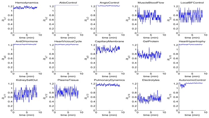
Evolution of δta;i (in min·10−3) for the main atomic models of the M2SL G72 implementation during the simulation of BM1, using time-synchronisation strategy ST3.
For ST2, although the values of δtc(t) = δta,i, ∀i are always slightly higher than in strategy ST1, computation times are similar to those obtained with that method (ratio of the simulation time with ST2/ST1 = 1.03). This is mainly due to the time consumed in estimating the smallest δta,i at each coupling instant. The mean-squared error obtained with this strategy, when compared to ST1 is 2.5285 · 10−5.
Concerning ST3, the value of δtc was fixed experimentally to 2.5 · 10−3 min. The heterogeneous dynamics of each atomic model can be appreciated in figure 8. Simulation under this configuration was 2.26 times faster than those observed with ST1 and the relative mean-squared error was 5.9385 · 10−4. The three strategies have also been applied to BM2, obtaining similar results.
(c). Integration of a pulsatile model of the heart
This section presents an example of vertical integration in which a module of the G72 model is replaced with a more detailed version. Indeed, the G72 model is based on a mean, non-pulsatile ventricular model and thus cannot be used for a beat-to-beat analysis. The integration of a new module representing an elastance-based pulsatile ventricle is thus explored.
Left and right ventricles on the original G72 model are represented by a simple AE, giving as output the ’baseline’ ventricle outflow (QLN and QRN for the left and right ventricles, respectively) for a given value of atrial pressure (PLA and PRA). The final ventricular outputs (QLO and QRO) are then computed as the product of QLN or QRN and various other parameters including the mean arterial pressure (PA), pulmonary pressure (PPA) and the autonomic effect on cardiac contractility (AUH).
In order to implement a pulsatile heart, the Guyton left heart model was substituted with a coupled model that includes two valves and a ventricle (figure 9-a). The heart valves are represented as non-ideal diodes, that correspond to modulated resistances. Each ventricle is modelled as a single time-varying elastance as poposed in previous studies (Guarini et al., 1998; Palladino and Noordergraaf, 2002). The main advantages of this approach are related to their low computational costs and the fact that they can easily be integrated into a model of the circulation. Time-varying elastances have shown a satisfying behaviour in response to physiological variations (change of position, temperature, physical activity, etc.) (Heldt et al., 2002). In order to model the ventricular contraction, a sinusoidal expression was used.
Figure 9.
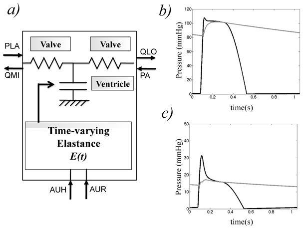
a) Implementation of the pulsatile left ventricle and valves. PLA(left atrial pressure), PA(arterial pressure), QLAO (ventricular inflow), QLO (ventricular outflow) b) Simulated pulsatile left ventricular pressure (black curves) and arterial pressure (grey curves) for one beat c) Simulated pulsatile right ventricular pressure (black curves) and pulmonary arterial pressure (grey curves) for one beat.
The pulsatile left ventricle and the valves were integrated into the hemodynamic block of the G72 model by connecting PLA and PA as inputs and the mitral and aortic flows (QMI and QLO) as outputs. The ventricle elastance is also connected to the autonomic control in order to take into account the regulation of heart rate (chronotropic effect) and ventricular contraction strength (inotropic effect). The output signal of the heart rate regulation model is continuous. To obtain pulsatile blood pressure, an IPFM (Integral Pulse Frequency Modulation) model was introduced (Rompelman et al., 1977). The input of the IPFM model is the Guyton variable for autonomic stimulation of heart rate (AUR). And each emitted pulse of the IPFM generates a variation of the ventricular elastance, which depends on AUH and AUR as follows:
| (3.1) |
where ta is the time elapsed since the last activation pulse; T is the contraction duration, which is modulated by the heart rate; Emin and Emax are respectively the minimum and the maximum value of the elastance function. Emax is modulated by AUH, as it is an indicator of ventricular contractility.
The implementation of the pulsatile right ventricle was done in a similar way, by using the right atrial pressure (PRA) and pulmonary arterial pressure (PPA) as inputs and flows through the tricuspid and pulmonary valves (QTR and QRO), as outputs.
Simulations were performed in steady-state conditions and during BM1, using ST3 for temporal synchronisation. The simulated pressure in steady-state shows realistic profiles for the left and right ventricles and the systemic and pulmonary arteries (figures 9-b and c). Figure 10 shows a comparison between the M2SL simulations of the original G72 model and the model coupled with pulsatile ventricles. A close match can be observed for PMO, QLO, BFM, MMO. Although the other curves are qualitatively consistent with original data, some differences can be noted for VUD, PVO, PA and AUP. This is mainly due to the fact that the pulsatile behaviour of the cardiac model generates oscillations on the other atomic models. It is important to note that an interface object, applying a mean value, could be used for input-output coupling between the pulsatile atomic models and their neighbours. Although this would avoid the above-mentioned problem, part of the benefit of including a pulsatile model would be lost. An additional parameter estimation stage could be applied to the proposed models in order to better approach all outputs.
Figure 10.
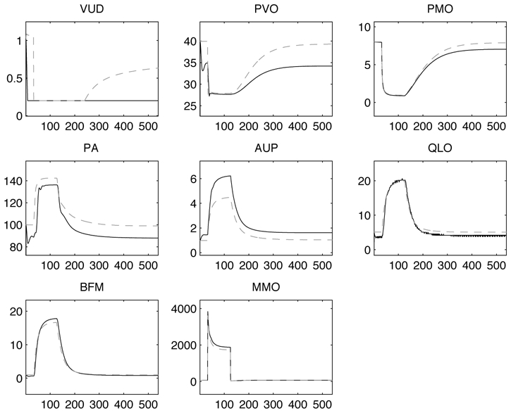
Comparison of M2SL simulations of Guyton model coupled with pulsatile ventricles (black curves) with the original Guyton model (dotted curves) during BM1 (sudden severe muscle exercise). Total experiment time was 9 min. VUD (urinary output in ml/min), PVO (muscle venous oxygen pressure in mm Hg), PMO (muscle cell oxygen pressure in mm Hg), PA (mean arterial pressure in mm Hg), AUP (sympathetic stimulation in ratio to normal), QLO (cardiac output in l/min), BFM (muscle blood flow, in l/min), and MMO (rate of oxygen usage by muscle cells in ml O2/minK1)
4. Discussion and Conclusions
This paper presented a multi-formalism modelling and simulation library, based on a co-simulation principle, that can be useful to perform an efficient model integration. This library provides an object-oriented environment to represent and solve coupled models, with components presenting different mathematical formalisms and heterogeneous dynamic properties.
The Guyton 1972 model was used as an example throughout the paper, as it presents interesting characteristics due to the modularity of its original presentation, the heterogeneity of the dynamics of each model component, and the potential to be used as a ’core model’ demonstrator, allowing for multi-resolution horizontal and vertical model integration. This model was implemented on M2SL as a coupled model made up of a set of atomic models, representing the main ’blocks’ proposed in the original paper. One fixed and two adaptive time-synchronisation strategies between atomic and coupled models (ST1 − ST3) have been proposed and evaluated. The two adaptive approaches are complementary in the way they can improve the efficiency of calculations. ST3 has shown to be particularly useful when the output variables used at the coupling stage are those presenting the slowest dynamics of their corresponding atomic models (or when an interface object performing a time-window mean operator is used at the interface of atomic and coupled models).
Although the results on this paper have been limited to the G72 model, the M2SL library has been in use for some years and other applications, coupling discrete (automata models) and continuous (Bond-Graph, ODE and transfer function) formalisms, have been presented elsewhere (Defontaine et al., 2005; Le Rolle et al., 2005). Moreover, an API is already available to couple M2SL models with external modules, and a parameter identification method, based on evolutionary algorithms, has been developed and applied to obtain patient-specific models in different biomedical contexts (Le Rolle et al., 2008; Wendling et al., 2005).
This library is still in active development. The lack of a graphical user interface (GUI) allowing to create M2SL models and to control simulations is one of the main current limitations. In addition to these GUIs, current developments include: i) a new time synchronisation strategy, integrating an adaptive coupling time-step as a function of the input-output dynamics of atomic models; ii) a set of XSLT transforms to support XML standards for model representation and iii) an MPI-compatible version of the library.
Acknowledgments
This work was supported by the INSERM and the French National Research Agency (ANR grant ANR-06-BYOS-0007-01 - SAPHIR Project). The authors would like to thank Ron White for providing access to benchmark data.
Footnotes
References
- Bassingthwaighte JB, Chizeck HJ, Atlas LE. Strategies and tactics in multiscale modeling of cell-to-organ systems. Proceedings of the IEEE. 2006;94:819–831. doi: 10.1109/JPROC.2006.871775. [DOI] [PMC free article] [PubMed] [Google Scholar]
- Blackett SA, Bullivant D, Stevens C, Hunter PJ. Open source software infrastructure for computational biology and visualization. Conf Proc IEEE Eng Med Biol Soc. 2005;6:6079–6080. doi: 10.1109/IEMBS.2005.1615879. [DOI] [PubMed] [Google Scholar]
- Defontaine A, Hernández A, Carrault G. Multi-formalism modelling of cardiac tissue. Lecture Notes in Computer Science - FIMH 2005. 2005;3504:394–403. [Google Scholar]
- Dou J, Xia L, Zhang Y, Shou G, Wei Q, Liu F, Crozier S. Mechanical analysis of congestive heart failure caused by bundle branch block based on an electromechanical canine heart model. Phys Med Biol. 2009;54:353–371. doi: 10.1088/0031-9155/54/2/012. [DOI] [PubMed] [Google Scholar]
- Fenner JW, Brook B, Clapworthy G, Coveney PV, Feipel V, Gregersen H, Hose DR, Kohl P, Lawford P, McCormack KM, Pinney D, Thomas SR, Jan SVS, Waters S, Viceconti M. The europhysiome, step and a roadmap for the virtual physiological human. Philos Transact A Math Phys Eng Sci. 2008;366:2979–2999. doi: 10.1098/rsta.2008.0089. [DOI] [PubMed] [Google Scholar]
- Fenton FH, Cherry EM, Karma A, Rappel WJ. Modeling wave propagation in realistic heart geometries using the phase-field method. Chaos. 2005;15:13502. doi: 10.1063/1.1840311. [DOI] [PubMed] [Google Scholar]
- Guarini M, Urzua J, Cipriano A. Estimation of cardiac function from computer analysis of the arterial pressure waveform. IEEE Transactions on Biomedical Engineering. 1998;45:1420–8. doi: 10.1109/10.730436. [DOI] [PubMed] [Google Scholar]
- Guyton A, Coleman T, Granger H. Circulation: overall regulation. Annu Rev Physiol. 1972;34:13–46. doi: 10.1146/annurev.ph.34.030172.000305. [DOI] [PubMed] [Google Scholar]
- Guyton A, Hall J. Textbook of Medical Physiology. New York: Saunders Co; 1995. Nervous Regulation of the Circulation, and Rapid Control of Arterial Pressure. [Google Scholar]
- Heldt T, Shim E, Kamm R, Mark R. Computational modelling of cardiovascular response to orthostatic stress. J Appl Physiol. 2002;92:1239–1254. doi: 10.1152/japplphysiol.00241.2001. [DOI] [PubMed] [Google Scholar]
- Hetherington J, Bogle I, Saffrey P, Margoninski O, Li L, Rey MV, Yamaji S, Baigent S, Ashmore J, Page K, Seymour R, Finkelstein A, Warner A. Addressing the challenges of multiscale model management in systems biology. Computers & Chemical Engineering. 2007;31:962–979. [Google Scholar]
- Hunter PJ. The IUPS Physiome Project: a framework for computational physiology. Prog Biophys Mol Biol. 2004;85:551–69. doi: 10.1016/j.pbiomolbio.2004.02.006. [DOI] [PubMed] [Google Scholar]
- Kerckhoffs RC, Neal ML, Gu Q, Bassingthwaighte JB, Omens JH, McCulloch AD. Coupling of a 3d finite element model of cardiac ventricular mechanics to lumped systems models of the systemic and pulmonic circulation. Ann Biomed Eng. 2007;35:1–18. doi: 10.1007/s10439-006-9212-7. [DOI] [PMC free article] [PubMed] [Google Scholar]
- Kofman E. Discrete event simulation of hybrid systems. SIAM Journal on Scientific Computing. 2004;25:1771–1797. [Google Scholar]
- Lara JD, Vangheluwe H. Fundamental Approaches to Software Engineering. Springer; 2002. ATOM 3: A Tool for Multi-Formalism Modelling and Meta-Modelling; pp. 174–188. [Google Scholar]
- Le Rolle V, Hernndez AI, Richard PY, Buisson J, Carrault G. A bond graph model of the cardiovascular system. Acta Biotheor. 2005;53:295–312. doi: 10.1007/s10441-005-4881-4. [DOI] [PMC free article] [PubMed] [Google Scholar]
- Le Rolle V, Hernndez AI, Richard PY, Donal E, Carrault G. Model-based analysis of myocardial strain data acquired by tissue doppler imaging. Artif Intell Med. 2008;44:201–219. doi: 10.1016/j.artmed.2008.06.001. [DOI] [PubMed] [Google Scholar]
- Loew LM, Schaff JC. The virtual cell: a software environment for computational cell biology. Trends in Biotechnology. 2001;19:401–406. doi: 10.1016/S0167-7799(01)01740-1. [DOI] [PubMed] [Google Scholar]
- McCulloch AD, Huber G. ’In silico’ simulation of biological processes. Wiley; 2002. Integrative biological modelling; pp. 4–19. [PubMed] [Google Scholar]
- Nickerson D, Niederer S, Stevens C, Nash M, Hunter P. A computational model of cardiac electromechanics. Conf Proc IEEE Eng Med Biol Soc. 2006;1:5311–5314. doi: 10.1109/IEMBS.2006.260169. [DOI] [PubMed] [Google Scholar]
- Noble D. Modeling the heart. Physiology (Bethesda) 2004;19:191–197. doi: 10.1152/physiol.00004.2004. [DOI] [PubMed] [Google Scholar]
- Palladino J, Noordergraaf A. A paradigm for quantifying ventricular contraction. Cell Mole Biol. 2002;7:331–335. [PubMed] [Google Scholar]
- Raymond G, Butterworth E, Bassingthwaighte J. Jsim: Free software package for teaching physiological modeling and research. Exper Biol. 2003;280:102. [Google Scholar]
- Rompelman O, Coenen AJ, Kitney RI. Measurement of heart-rate variability: Part 1-comparative study of heart-rate variability analysis methods. Med Biol Eng Comput. 1977;15:233–239. doi: 10.1007/BF02441043. [DOI] [PubMed] [Google Scholar]
- Thomas SR, Baconnier P, Fontecave J, Franoise JP, Guillaud F, Hannaert P, Hernndez A, Rolle VL, Mazire P, Tahi F, White RJ. Saphir: a physiome core model of body fluid homeostasis and blood pressure regulation. Philos Transact A Math Phys Eng Sci. 2008;366:3175–3197. doi: 10.1098/rsta.2008.0079. [DOI] [PubMed] [Google Scholar]
- Tomita M. Whole-cell simulation: a grand challenge of the 21st century. Trends Biotechnol. 2001;19:205–210. doi: 10.1016/s0167-7799(01)01636-5. [DOI] [PubMed] [Google Scholar]
- Usyk TP, McCulloch AD. Relationship between regional shortening and asynchronous electrical activation in a three-dimensional model of ventricular electromechanics. J Cardiovasc Electrophysiol. 2003;14:S196–S202. doi: 10.1046/j.1540.8167.90311.x. [DOI] [PubMed] [Google Scholar]
- Vangheluwe H, de Lara J, Mosterman PJ. An introduction to multi-paradigm modelling and simulation. Proceedings of the AIS’2002 Conference; 2002. pp. 9–20. [Google Scholar]
- Watanabe H, Sugiura S, Kafuku H, Hisada T. Multiphysics simulation of left ventricular filling dynamics using fluid-structure interaction finite element method. Biophys J. 2004;87:2074–2085. doi: 10.1529/biophysj.103.035840. [DOI] [PMC free article] [PubMed] [Google Scholar]
- Wendling F, Hernndez A, Bellanger JJ, Chauvel P, Bartolomei F. Interictal to ictal transition in human temporal lobe epilepsy: insights from a computational model of intracerebral EEG. J Clin Neurophysiol. 2005;22:343–356. [PMC free article] [PubMed] [Google Scholar]
- Zeigler BP, Praehofer H, Kim TG. Integrating Discrete Event and Continuous Complex Dynamic Systems. 2. Academic Press; 2000. Theory of Modeling and Simulation. [Google Scholar]