

Abstract
A new sharp-interface immersed boundary method based approach for the computation of low-Mach number flow-induced sound around complex geometries is described. The underlying approach is based on a hydrodynamic/acoustic splitting technique where the incompressible flow is first computed using a second-order accurate immersed boundary solver. This is followed by the computation of sound using the linearized perturbed compressible equations (LPCE). The primary contribution of the current work is the development of a versatile, high-order accurate immersed boundary method for solving the LPCE in complex domains. This new method applies the boundary condition on the immersed boundary to a high-order by combining the ghost-cell approach with a weighted least-squares error method based on a high-order approximating polynomial. The method is validated for canonical acoustic wave scattering and flow-induced noise problems. Applications of this technique to relatively complex cases of practical interest are also presented.
Keywords: Immersed Boundary Method, Computational Aeroacoustics, Flow induced noise, Phonation
1. Introduction
Low-Mach number, flow-induced sound plays a critical role in engineering applications such as transportation systems, engineering appliances and turbo-machines. In many of these applications, flow-induced noise is undesirable and engineers seek to identify noise source(s) with the objective of eliminating or diminishing the same. One examples of this is the cabin noise in automobiles associated with external air-flow and another is the aeroacoustics sound associated with the flow from an air-conditioning vent. Flow-induced sound also plays an important role in biomechanics. Human speech and animal vocalization is enabled by the generation of flow-induced sound in the larynx [1]. In the cardiovascular system, sounds such as “bruits” [2], heart murmurs[3], and Korotkoff sounds [4] are blood-flow induced sounds that carry important information about the health of the individual. Finally, hydroacoustic sound generation[5, 6, 7] associated with wakes, shear layers, jets, tip-vortices etc. are also low-Mach number flows phenomena which have tremendous importance in naval hydrodynamics and ocean acoustics.
The ability to predict flow-induced sound in these various applications can advance the design of quieter devices/machines and also lead to insights and non-invasive diagnostic techniques for pathologies associated with phonation, speech and the cardiovascular system. However, all of the above aeroacoustic problems are associated with very complex geometries, and accurate prediction of sound generation and propagation in such complex geometries is a challenging proposition. Although sound wave propagation and scattering by a complex geometry can be modeled with a boundary element method (BEM) [8, 9], the prediction of flow induced sound generation requires more direct approach such as the direct computation of compressible conservation equations (see [10, 11]). Computation of sound wave generation/propagation requires a method that has very low dispersion and dissipation and is therefore best accomplished by high-order finite-difference schemes such as compact schemes [12] or DRP (Dispersion-Relation-Preserving) scheme [13]. Most of these high-order, finite-difference numerical method used in computational aeroacoustics (CAA) are formulated on structured grids and are usually very sensitive to the quality of the computational grid and the formulation of the boundary conditions. However, it is difficult to generate high-quality structured grids around complex geometries and this has mostly limited CAA to relatively simple geometries.
There are however a few approaches that have been used with some success for CAA in relatively complex geometries. A high-order overset grid method[14, 15] has been developed to solve the compressible flow and acoustics over complex geometries. However the level of geometric complexity that this solver can handle is still limited. Furthermore, while the method is well suited for high-Mach number sound, computations at low Mach numbers (M < 0.1) are difficult. The high-order discontinuous Galerkin method[16, 17, 18, 19] could be an alternative to solve for the aeroacoustic field around complex geometries, but this method is computationally expensive. Thus, there is a clear need for developing a method that can compute low-Mach number flow-induced sound in geometrically complex configurations.
The immersed boundary method (IBM)[20] is well suited for dealing with complex geometries. With IBM, all the equations can be solved on a body non-conformal, Cartesian grid, and also the grid does not need to be re-generated for moving or deforming bodies. Due to this flexibility, many different types of IBM are used in compressible and incompressible flow solvers. A few IB based approaches for acoustic wave propagation/scattering problem in frequency [21, 22] and time domain[23, 24] have also been developed. In these studies, however, only the linear wave propagation and scattering with prescribed acoustic source is considered. The key to IBM is the treatment of boundary condition at the body surface and the vast majority of immersed boundary formulation are first or second-order accurate (one exception is the high-order immersed-interface method of Linnick[25]). For example, in the IB method of Tullio et al.[26] and Palma et al.[27] for compressible flows, a direct forcing with a linear or inverse-distance weighted interpolation is employed and this leads to a locally first-order accurate method. In the compressible IB method of Ghias et al.[28], a ghost-cell method is used with two-point centered scheme, which results in local and global second-order accuracy.
Acoustic field computations however require high-order boundary formulations so as to minimize the dispersion/dissipation errors. Additionally, not only the order of accuracy of boundary formulation, but also the sharpness of interface would be very important in order to limit the phase and amplitude errors generated by a wave interacting with the boundary. Recently, Liu & Vasilyev[29] applied a Brinkman penalization method, which is an immersed boundary method based on a porous media model equation, to the compressible Navier-Stokes equations and considered an acoustic wave scattering problem. Although the order of accuracy of numerical scheme could be maintained near the immersed boundary, the immersed interface is not sharp.
In the present study, we propose a sharp-interface, higher-order immersed boundary method to solve aeroacoustic problems with complex bodies in low-Mach number flows. For the efficient computation of low Mach number aeroacoustics, a hybrid method based on the hydrodynamic/acoustic splitting technique [30, 31, 32] is employed. In this approach, the flow field is obtained by solving the incompressible Navier-Stokes equations (INS), and the acoustic field is predicted by the linearized perturbed compressible equations (LPCE) proposed by Seo & Moon[32]. The INS/LPCE hybrid method is a two-step/one-way coupled approach to the direct simulation of flow induced noise. In the method proposed here, we couple an existing immersed boundary solver for incompressible flows[33] with a new high-order immersed boundary method for solving the LPCE equations with complex immersed boundaries. The high-order immersed boundary method proposed here also employs ghost-cells as in Refs.[28, 33] but the method is extended to higher-orders by using an approximating polynomial method originally proposed by Luo et al.[34] for the solid mechanics equations. Dirichlet as well as Neumann boundary conditions can be applied with a high order of accuracy on the solid surface using the method. Thus dispersion/dissipation errors caused by the boundary condition formulation can be minimized thereby ensuring highly accurate representation of wave reflection on the solid walls.
The current method therefore combines the flexibility of the immersed boundary method with the capability offered by the INS-LPCE hydrodynamic/acoustic splitting technique for computing low Mach number (M < 0.3) flow-induced sound. It should be pointed out that the sound generation and propagation is modeled here in a natural way and unlike acoustic analogy methods (e.g. Lighthill's analogy[35]), the predicted acoustic field is valid for both the far and near-fields. The time-dependant base flow effects on the sound generation and propagation are also fully taken into account. Additionally, the LPCE secures a consistent acoustic solution by suppressing the evolution of the unstable perturbed vortical mode[32]. Finally, since this method is based on the incompressible flow solution, it is very effective for the flows at low Mach numbers which are of particular relevance to the applications of interest to us.
The paper is organized as follows: In section 2, the governing equations and numerical methods including the present immersed boundary approach are described. In section 3, several canonical acoustic wave scattering problems and a fundamental flow-induced noise problem are considered in order to validate the present method. The acoustic wave scattering results are compared with analytical solutions while the flow-induced noise simulation is validated against data from a highly resolved direct compressible flow simulation performed on a body-fitted grid using a different solver. Finally, the capability of the present approach for modeling flow-induced sound in complex geometries is demonstrated by computing the generation and propagation of sound in a modeled human vocal-tract as well as that from a modeled air-conditioning vent.
2. Computational Method
2.1. Governing Equations
In the hydrodynamic/acoustic splitting method, the total flow variables are decomposed into the incompressible variables and the perturbed compressible ones as:
| (1) |
where ρ0, U⃗, P are the incompressible flow density (constant), velocity, pressure, and ρ′, u⃗′, p′ are compressible perturbed counter parts. The incompressible variables predicted by the incompressible Navier-Stokes equations represent the hydrodynamic flow field, while the acoustic fluctuations and other compressibility effects are represented by the perturbed quantities denoted by (′). The incompressible Navier-Stokes equations are written as
| (2) |
| (3) |
The equations for the perturbed quantites (i.e. the perturbed compressible equations (PCE)[31]) can be derived by subtracting the incompressible Navier-Stokes equations from the compressible ones with the variable decomposition, Eq. (1). The PCE, however, contains the perturbed vortical mode (ω⃗′ = ∇ × u⃗′) generated by the coupling effect between perturbed velocities and hydrodynamic vorticity. While this may be not a major sound source at low Mach numbers, it can cause a self-excited instability if not properly resolved[32]. A detailed order-of-magnitude analysis of the equation that governs this quantity[32] shows that all the source terms are O(M4) which are clearly smaller than the O(M) terms retained in the linearization process. Therefore, this term can be safely dropped from the linearized equations. A resulting set of linearized perturbed compressible equations (LPCE) can be written in a vector form as,
| (4) |
| (5) |
| (6) |
where s′ is any additional prescribed acoustic source. The boundary conditions on the solid wall are:
where n̂ is the unit wall-normal vector, and the initial conditions are normally ρ′ = u⃗′ = 0 and . It should be noted that the LPCE has a much simpler form than the original PCE. Furthermore, the perturbed velocity (Eq. 5) and pressure (Eq. 6) fields are decoupled from the perturbed density field (Eq. 4), and if one is not interested in a perturbed density field, this equation does not need to be solved. The left hand sides of LPCE represent the effects of acoustic wave propagation and refraction in the unsteady, inhomogeneous base flows, while the right hand side only contains the acoustic source term. For low Mach number flows, it is interesting to note that the total change of hydrodynamic pressure DP/Dt is the only source term coming from the incompressible base flow and this is consistent with the analysis of Goldstein[38]. The LPCE have been well validated for fundamental dipole/quadruple flow noise problems[32] and also for the low Mach number turbulent flow noise problems[36, 37]. Further details regarding the derivation of LPCE can be found in Ref.[32].
2.2. Numerical Methodology
The underlying flow equations for the base flow are the incompressible Navier-Stokes equations (Eqs. 2 and 3) and these are solved with a projection method based approach[39]. A second-order central difference is used for all spatial derivatives and time integration is performed with the second-order Adams-Bashforth method for convection terms and Crank-Nicolson method for diffusion terms[33].
The LPCE are spatially discretized with a sixth-order central compact finite difference scheme[12] and integrated in time using a four-stage Runge-Kutta (RK4) method[40]. The first derivative is evaluated with a sixth-order compact scheme as follows
| (7) |
where α = 1/3, a = 14/9, and b = 1/9. Near the immersed solid boundaries and domain boundaries, the following boundary schemes are used.
| (8) |
| (9) |
Equation (8) is fourth-order and (9) is third-order accurate. These boundary schemes are discussed and suggested in Ref.[12]. Since a central compact scheme has no numerical dissipation, an implicit spatial filtering proposed by Gaitonde et al.[41] is applied to suppress aliasing errors and ensure numerical stability. A general M-th order spatial filtering formulation is written as
| (10) |
where −0.5 < αf < 0.5 is a free parameter, and coefficients an can be found in Ref.[41]. For a value of αf which is close to 0.5, the filtering truncates only very high wave number components. In this study, we applied tenth-order filtering with αf = 0.45 in the interior region. Near the boundaries, reduced, (8th, 6th, 4th, and 2nd) order filtering is used. A similar approach is used in the high-order, body-fitted compressible flow solver in Ref.[42]. The spatial derivative, Eq. (7)-(9), and filtering, Eq. (10) form a closed tri-diagonal matrix system. Thus, the spatial derivative and filtering are computed by a usual tri-diagonal matrix solver algorithm (e.g. Thomas algorithm[43]). For the non-uniform Cartesian grid, the physical derivatives are evaluated by the following transformation:
| (11) |
where xi and ξi are coordinates for physical and computational domain, respectively. The metric, with the high-order numerical schemes described above to retain the order of accuracy[42]. Once the spatial derivatives are evaluated, the LPCE system is solved by a fully explicit four stage Runge-Kutta time-marching scheme[40] and the spatial filtering is applied at the end of each time-step.
2.3. Immersed Boundary Formulation
The incompressible Navier-Stokes equations for the base flow with complex immersed boundaries are solved using the sharp-interface immersed boundary method of Mittal et al.[33]. In this method, the surface of the immersed body is represented with an unstructured surface mesh which consists of triangular elements. At the pre-processing stage before integrating governing equations, all cells whose centers are located inside the solid body are identified and tagged as ‘body’ cells and the other points outside the body are ‘fluid’ cells. Any body-cell which has at least one fluid-cell neighbor is tagged as a ‘ghost-cell’ (see Fig. 1), and the wall boundary condition is imposed by specifying an appropriate value at this ghost point. In the method of Mittal et al.[33] a ‘normal probe’ is extended from the ghost point to intersect with the immersed boundary (at a body denoted as the ‘body intercept’). The probe is extended into the fluid to the ‘image point’ such that the body-intercept lies midway between the image and ghost points. A linear interpolation is used along the normal probe to compute the value at the ghost-cell based on the boundary-intercept value and the value estimated at the image-point. The value at the image-point itself is computed through a tri-linear (in 3D) interpolation from the surrounding fluid nodes. This procedure leads to a nominally second-order accurate specification of the boundary condition of the immersed boundary.
Figure 1.

Schematic of ghost cell method
While the above normal-probe approach is well suited for achieving second-order accuracy, extension to higher order formulations is problematic. Higher-order formulations require large interpolation stencils along the normal probe and for complex geometries, these large stencils can intersect with other nearby immersed boundaries (see Fig 2b). Also, the overall accuracy could be limited by the interpolation method used to compute values on the image points. A method is therefore needed which will enable higher-order boundary formulations while allowing a high degree of flexibility with respect to the interpolation stencil. In the current approach we propose the use of high-order polynomial interpolation combined with a weighted-least square error minimization. In this approach, the value at the ghost point is determined by satisfying the boundary condition at the body-intercept point using high-order polynomial. Specifically, a generic variable ϕ is approximated in the vicinity of the body-intercept point (xBI, yBI, zBI) in terms of a Nth-degree polynomial Φ as follows:
Figure 2.

Schematic of the boundary condition formulation
| (12) |
where x′ = x − xBI, y′ = y − yBI, z′ = z − zBI and cijk are unknown coefficients. In fact, Eq. (12) is the approximation of ϕ using the Taylor series expansion from the body-intercept point:
| (13) |
where subscript ‘BI’ denotes the value at the body-intercept point (xBI, yBI, zBI). The coefficients, cijk can be expressed as
| (14) |
The number of coefficients L for a polynomial order N is listed in Table 1 for 2D and 3D cases. In order to determine these coefficients, we need values of ϕ from fluid data points around the body-intercept point. Following Luo et al.[34], a convenient and systematic method for selecting these data points is to search a circular (spherical in 3D) region (of radius R) around the body-intercept point. (see Fig. 2). With M such data points, the coefficients cijk can be determined by minimizing the weighted error estimated as:
Table 1. Number of coefficients (L) for N-th order polynomial.
| L(N) | ||
|---|---|---|
| N | 2D | 3D |
| 1 | 3 | 4 |
| 2 | 6 | 10 |
| 3 | 10 | 20 |
| 4 | 15 | 35 |
| (15) |
where is the m-th data point, and wm is the weight function. In this study, we used a cosine weight function suggested in previous studies[34, 44]:
| (16) |
where is the distance between the m-th data point and the body-intercept point. To make the least-square problem well-posed, M > L(N) and the radial range R is adaptively chosen so as to ensure the satisfaction of this well-posedness condition. Since we need to find the value at the ghost point in conjunction with the body-intercept point, the first data point is replaced by the ghost point, and (M − 1) data points are found in fluid region (see Fig. 2). The exact solution of the least-square error problem, Eq. (15) is given by
| (17) |
where superscript ‘+’ denotes the pseudo-inverse of a matrix, vector c and ϕ contain coefficients cijk and the data respectively, and W and V are the weight and Vandermonde matrices given by
| (18) |
Note that is the ghost-point and V is a M × L matrix where L is the number of coefficients listed in Table 1. The pseudo-inverse matrix is computed by singular value decomposition (SVD) method[45]. After solving Eq. (17), the coefficients cijk can be written as a linear combination of . For example,
| (19) |
where A(l, m) is the l-th row, m-th column component of matrix A = (WV)+W, which has dimension of L × M. According to Eq. (13), coefficients cijk represent the value and derivatives at the body-intercept point (xBI, yBI, zBI):
| (20) |
Therefore, for given Dirichlet or Neumann type boundary condition at the body wall, the value at the ghost point can be evaluated with Eq. (19) & (20). For example, given the Dirichlet boundary condition at the wall, ϕ(xBI, yBI, zBI) = φw, the value at the ghost-point can be computed as
| (21) |
where φgp is the value at the ghost point . For the Neumann type boundary condition, , the value at the ghost point is given by
| (22) |
where n̂ is the unit wall normal vector at the body point.
The present method allows a high level of flexibility with respect to the choice of the stencil points. One essentially needs to find a sufficient number of fluid points around the body-intercept point to accomplish the interpolation and the simplest procedure is to increase the radius R until the required number of fluid interpolation points are identified (see Fig 2b). The key to successful implementation of this method is to maintain the well-posedness of the least-square error problem, Eq. (17), and a convenient way to check this is to monitor the condition number of matrix (WV). Large values of the condition number are indicative of an ill-conditioned situation which has to be remedied by increasing the number of data points in the stencil. It is found that the condition number is dependent on the geometrical configuration and the order of polynomial. In most case, the matrix (WV) is singular, and it means that one can not get a well-posed condition with the minimum number of data points, i.e. M = L(N). Even though the least-square error problem is successfully solved with the SVD technique, (Eq. 17), for large condition number of (WV) (e.g. O(106) or larger), small numerical errors in the ghost-point value can amplify and lead to numerical instability. Thus it is necessary to limit the maximum condition number by increasing the number of data points used in the interpolation. Note that even for large interpolation stencils, the computational expense associated with the implementation of the boundary condition is a small fraction of the overall expense since the number of ghost cells is a very small proportion of the total number of cells in the computational domain. Also, the search for the data points and matrix computations for each ghost-point is done once at in the pre-processing stage and the matrix A = (WV)+W is stored at that time. The computation for the value on the ghost point at every time step is then accomplished through highly efficient vector multiplications (Eq. 21 and 22).
Once the boundary condition is imposed by setting the ghost-point value, the values at the internal body points need not to be computed and these points are treated as holes in computational domain. For spatial derivative and filtering, the body points are decoupled in the tri-diagonal matrix system by setting banded values as {0 1 0}. To close the tri-diagonal matrix system, the same boundary derivative and filtering scheme used at the domain boundary are also applied at the immersed boundary. Near the immersed body interface, spatial derivative and filtering scheme are applied as shown in Fig. 3. Here C6, C4 and C3 indicate Eq. (7), (8), and (9) respectively, and FP denotes P-th order spatial filtering. Note that the first point of spatial derivative formulation is the ghost-point, but this point is not filtered to ensure accurate specification boundary condition. The present boundary derivative and filtering schemes are chosen by considering the stability and flexibility of the overall method. We have found that one-sided higher-order derivative/filtering schemes[46, 47] are unstable for the current method. This may be because the ghost-point value is not determined one-dimensionally along the numerical stencils. Furthermore, such one-sided schemes require extended one-sided numerical stencils which would degrade the overall flexibility of the method, since such stencils can intersect with other nearby immersed boundaries. On the other hand, the present method can potentially work even when the distance between two immersed boundaries is relatively small. While the most satisfactory solution to computing flows with small gaps is to improve resolution (such as with local refinement), sometimes the flow in these regions might be of marginal interest and the present method would be particularly useful for such cases.
Figure 3.

Application of compact scheme and spatial filtering near the immersed boundary
3. Results and Discussion
In order to test the present immersed boundary method and boundary condition formulation for the LPCE equations, several benchmark 2D and 3D problems in acoustic scattering are considered. Following this, we validate our computed solution for sound generation by a cross flow over a circular cylinder against that obtained from a highly accurate direct simulation of the full compressible flow equations. Finally, we demonstrate the versatility of the current approach by computing flow-induced sound in two complex configurations with widely disparate appications: one in biomechanics and the other in engineering acoustics.
3.1. Acoustic Wave Scattering Bench-Mark Problems
In order to test the present immersed boundary method and boundary condition formulation, several benchmark problems are considered. The first problem is the acoustic wave scattering by a circular cylinder (Fig. 4) which is a well established validations case[22, 29, 49]. A circular cylinder with diameter 1 is placed at (x, y) = (0, 0), and the computational domain is −6 ≤ (x, y) ≤ 6. The Gaussian pulse at (x, y) = (4, 0) is given by the initial condition,
Figure 4.

Schematic of benchmark problem: acoustic wave scattering by a circular cylinder
| (23) |
Equations (5)-(6) are solved with U = 0, P = 1/γ on a (600 × 600) uniform Cartesian grid with Δx = Δy = 0.02, and a time step Δt = 0.01 is used. At the cylinder surface, a slip-wall boundary condition is applied for the perturbed velocities, and the Neumann boundary condition of wall-normal gradient zero is applied for the perturbed pressure. For outer boundaries, the ‘Energy Transfer and Annihilating (ETA)’ boundary condition [48] is used to treat the out-going acoustic waves. For the immersed boundary formulation, N = 3 (third-order polynomial) and M = 40 are used. As discussed above, the maximum number of data points, M should be chosen so that the least-square error problem is well-posed. We have found that the current numerical method is stable for the maximum condition number of matrix (WV) (in Eq. 17) up to O(105), and the number of data points M = 40 (about 6 × 6 grid points, if approximated as a square array stencil in 2D) is required to get such well-posed condition for the present configuration. Note that this stencil size (about 6 along the grid line) is very much inline with the stencil of the sixth-order compact scheme (5 along the grid line). As mentioned earlier, the number of data points used in the approximation does not significantly increase the overall computational time. For this particular case, the computation time for the pre-processing step was about 10% of one time-step of the flow computation and the computation time for the applying immersed boundary condition was about 0.1% of the overall computation time.
The time evolution of the acoustic wave is shown in Fig. 5 and reflected as well as deflected waves are observed. The time histories of pressure fluctuation monitored at four different positions around a cylinder (point a-d in Fig. 4) are plotted in Fig. 6 along with the analytical solution[49]. We note that the computed results agree very well with the analytical solution.
Figure 5.

Acoustic wave scattered by a circular cylinder. Perturbed pressure, p′ contours (10 contour levels between -0.04 and 0.04)
Figure 6.

Time histories of pressure fluctuation compared with analytical solutions. Sold line: present, Dash-dot: analytical solution
We use this case to perform a convergence test of the present immersed boundary method. The convergence test employs five different grid sizes with Δx = Δy ranging from 0.02 to 0.08. The results with Δx = 0.02, 0.04, and 0.08 are plotted along with the analytical solution in Fig. 7a for the first reflected wave monitored at point a(x = 2, y = 0). The result with a grid spacing, Δx = 0.04 is still acceptable, while the coarser grid, Δx = 0.08 causes noticeable reduction in the peak value. It should however be noted that with Δx = 0.08, the cylinder is resolved by only about 12 grid points which explains the loss in accuracy. The grid convergence rate is analyzed by the error with respect to the analytical solution at the peak time for the incident and (first) reflected wave at point a, respectively. Since the error is computed at a fixed time, it addresses both phase and amplitude error. The results are shown in Fig. 7b for different polynomial orders of immersed boundary formulation, N = 1 ∼ 4. Since the incident wave is not affected by immersed-boundary formulation, it shows a clear sixth-order convergence. The error clearly increases for the reflected wave due to influence of the boundary schemes (reduced-order discretization/filtering near the boundary) and the immersed boundary formulation. It is observed that the absolute error is smaller for the higher polynomial order, N, but the slope of convergence is similar for all N except the linear method (N = 1). The result with N = 4 is not much different with N = 3. The convergence slope is about five for the finer grid resolution, but it degrades to about three for the coarser resolutions. This might be due to the fact that the present boundary scheme is only third-order accurate at the ghost point, and the ratio of number of ghost points to the number of interior fluid points along the grid line is larger for the coarser resolution. However, the fast (nearly 5th order) convergence at relatively finer grid resolutions is very encouraging and quite acceptable for most aeroacoustic problems. From a practical point-of-view, the increased error level due to the boundary formulation can be controlled with a non-uniform grid clustering around the immersed boundaries.
Figure 7.

a) Time histories of pressure fluctuation at (x, y) = (2, 0) for the first reflected wave. Symbols: analytical solution. b) Errors for the incident wave (black line, circular symbols) and the first reflected wave (other lines). Errors are computed for the time signal at (x, y) = (2, 0) with respect to the analytical solution at the peak time.
In the second test problem, the initial acoustic pulse is replaced by a time harmonic, Gaussian monopole source:
| (24) |
where ω = 8π, b = 0.2, and (x0, y0) = (4, 0). All other conditions are the same with the first problem. The snapshot of acoustic field around a cylinder is shown in Fig. 8a and the directivity of at r = 0.52 (which is very near the immersed boundary) and r = 5 are plotted along with the analytical solution[49] in Fig. 8b and c. The present result agrees very well with the analytical solution at both locations. Higher frequency wave scattering is also considered with ω = 12π and 16π. For these cases, b is set to 0.1 and the grid spacing and time step size are 0.01 and 0.005, respectively. The directivity of at r = 5 is found to compare well with the analytical solution in Fig. 9 and thus high-frequency wave scattering is also resolved well by the present immersed boundary method.
Figure 8.
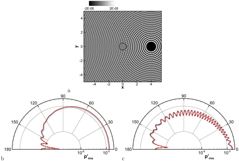
Time-harmonic acoustic wave scattering. a) Snapshot of fluctuating pressure field, b) directivity of at r = 0.52, c) at r = 5. sold line: analytical solution, symbols: present.
Figure 9.

High-frequency time-harmonic acoustic wave scattering. Directivity of at r = 5. a) ω = 12π, b) ω = 16π. sold line: analytical solution, symbols: present.
Now in order to test a complex geometrical configuration, the acoustic wave scattering by three cylinders with different sizes is considered[50]. The time harmonic monopole source defined by Eq. (24) is placed at the origin, (x0, y0) = (0, 0) and source parameters are set to b = 0.2, ω = 8π. The computational domain is −8 ≤ (x, y) ≤ 8, and a uniform Cartesian grid with Δx = 0.02 is used. The first cylinder with diameter 1 is placed at (−3, 0) and two cylinders with diameter 0.75 are placed at (3, −4) and (3, 4). Figure 10a shows the instantaneous fluctuating pressure field, and profile along the y = 0 line is compared with the analytical solution[50] in Fig. 10b and c. We note that the present results coincide well with the analytical solution thereby demonstrating the ability of the the solver to provide accurate solution with relatively complex geometries.
Figure 10.
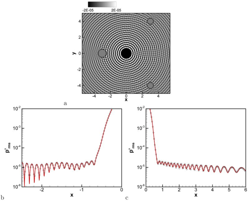
Acoustic wave scattering by three cylinders. a) Snapshot of fluctuating pressure field. along the y = 0 line, b) from the source to the surface of left cylinder, c) from the souece to the center of two right cylinders. Sold line: analytical solution, symbols: present.
Finally, we consider a three-dimensional acoustic wave scattering problem. A sphere with diameter 1 is placed at (x, y, z) = (0, 0, 0), and a Gaussian monopole source is given by,
| (25) |
The frequency ω is set to 6π. A uniform Cartesian grid of 400 × 200 × 200 (16 million) with grid spacing 0.03 is used and the time step is set to Δt = 0.01. For the immersed boundary formulation, N = 3 and M = 80 are used. The present LPCE solver is fully parallelized by the domain decomposition technique using a message passing interface (MPI) library, and the current Cartesian grid is easily and efficiently decomposed into 8 × 4 × 4 (128) blocks. One time-step takes about 7 sec. with 128 processors on the NICS-Kraken (Cray XT-5). The instantaneous perturbed pressure field is shown in Fig. 11a and the directivity of at r = 2 on z = 0 plane plotted along with the analytical solution [51] in Fig. 11b shows excellent agreement.
Figure 11.
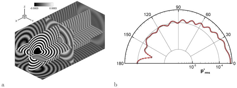
Spherical, time-harmonic wave scattering. a) Snapshot of fluctuating pressure field, b) directivity of at r = 2 on z = 0 plane, sold line: analytical solution, symbols: present.
3.2. Flow Induced Noise
The present method is now applied to an actual low Mach number flow-induced noise problem: the generation of tonal noise by the flow past a circular cylinder. The Reynolds number based on a cylinder diameter D, ReD = U∞D/ν is 200 and Mach number M = U∞/c = 0.2. Here U∞, c, and ν are free-stream flow velocity, speed of sound, and kinematic viscosity, respectively. The incompressible flow field is solved by the immersed boundary incompressible flow solver, developed by Mittal et al.[33] and described briefly in Sec 2. The domain size for the simulation is −90D ≤ x ≤ 90D, −100D ≤ y ≤ 100D and a non-uniform 512 × 512 Cartesian grid with Δxmin = Δymin = 0.015D is used (see Fig. 12). The grid is stretched in the outer region and the maximum grid spacing is about 1.4D. The grid resolution in the far-field is designed to resolve only acoustic waves. For the present case, the acoustic wave length is expected to be about 25D and this wave length is resolved by about 20 grid points in the far-field. The time step for the flow simulation is set to Δtf = 0.005D/U∞. For this particular case, the associated LPCE are solved on the same Cartesian grid as the flow solver. However, it should be noted that in principle, the two grids can be different and that would necessitate a spatial interpolation of the base flow terms employed in the LPCE equations. For the flow solver, the viscous flow sturucture should be resolved accurately with the refined grid resolution around the immersed body. In this regard, a local grid refinement strategy would be quite helpful in increasing the efficiency of the present immersed boundary flow solver. For the LPCE simulation, Δta = Δtf/3 is used in order to satisfy the acoustic CFL condition, cΔta/Δx ≤ 1, and the base flow U, P and source term DP/Dt are obtained by a second-order temporal Lagrangian interpolation of the incompressible flow solution. Thus, for tf < ta ≤ tf + Δtf, the incompressible flow solutions at three time levels (tf − Δtf, tf, tf + Δtf) are used for the Lagrangian interpolation. Since the current flow solver is second-order accurate in time, this temporal interpolation method is sufficient to retain the overall temporal accuracy of the solver. Both the flow and the acoustic solvers are fully parallelized and computations are carried out simultaneously. On 16 processors of an IBM iDataPlex cluster, the computation of one time step takes about 6 sec. for the flow solver and about 1 sec. for the acoustic solver.
Figure 12.

Computational grid around a circular cylinder
Figure 13 shows the instantaneous vorticity field obtained by the immersed boundary incompressible flow solver and time histories of the drag and lift coefficients. Karman vortex shedding is observed in the cylinder wake and the computed Strouhal number is St = fD/U = 0.195 which matches well with the value of 0.196 reported in the literature[52]. The computed mean drag coefficient CD,avg = 1.31 is also very close to the value of 1.33 obtained by Henderson[53]. Figure 14a shows the acoustic field solved by LPCE on the same Cartesian grid. The acoustic field is visualized by time fluctuation of total pressure:
Figure 13.
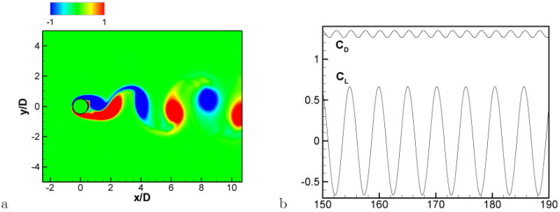
a) Instantaneous vorticity field (immersed boundary incompressible flow solver), non-dimensionalized by U/D. b) Time histories of drag and lift coefficients.
Figure 14.
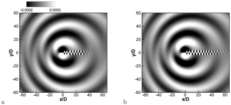
Comparison of instantaneous acoustic field; instantaneous pressure fluctuation contours, non-dimensionalized by ρ0c2. a) Incompressible Navier-Stokes/LPCE hybrid method on the Cartesian grid. b) Direct simulation of compressible Navier-Stokes equations on the body-fitted, O-type grid.
| (26) |
where overbar denotes time average and one can clearly observe the dipole noise generated by periodic vortex shedding. For comparison, the problem has also been solved by a direct numerical simulation (DNS) on an O-type body-fitted grid. In this simulation, the full compressible Navier-Stokes equations are solved on the cylindrical grid using a high-order numerical scheme (a sixth-order compact scheme for spatial derivatives, and a four-stage Runge-Kutta method for time integration) and both flow and acoustics are resolved simultaneously[31, 32]. The outer domain boundary of the grid lies at r = 100D and the grid employs 400 and 640 points in the circumferential and radial directions respectively. The minimum grid spacing in this DNS is 0.005D and the results are compared in Fig. 14 and 15. The instantaneous acoustic field obtained by the direct simulation shown in Fig. 14b is almost the same with the one predicted by the present method. It is however observed that the vortical structure in the wake is damped out earlier in the present result than the compressible DNS. This is because the spatial derivative scheme used in the present flow solver is second-order accurate, while the DNS employs a sixth-order scheme. Furthemore, the stream-wise grid resolution is finer for body-fitted DNS. However, these convecting/diffusing vortices at the far-downstream are not a significant noise source, and therefore do not affect the accuracy of acoustic field in other regions. In Figure 15, the pressure fluctuation Δp′ along the x = 0 line above the cylinder and along a line inclined 30 degree from the wake are plotted for both direct simulation and the present method and one can see that the present result matches well with the direct simulation.
Figure 15.

Pressure fluctuation Δp′, a) along the x = 0 line above the cylinder, b) along a line inclined 30 degree from the wake (x-axis). black solid line: present result (immersed boundary INS/LPCE hybrid method on a Cartesian grid), red circular symbols: the result of direct simulation performed on a body-fitted grid.
3.3. Generation and Propagation of Voiced Sound in the Human Vocal Tract
The present method is now applied to the computation of voiced sound generation and propagation to demonstrate its capability for dealing with complex geometries in practical applications. Human phonation and speech is well suited for the current methodology since it involves low-Mach number flow induced sound in a complex geometry. It is well known that the source of voiced sound is the flow rate fluctuation in the vocal tract caused by the vibration of vocal folds in the larynx[54]. The glottal flow rate fluctuation generates monopole sound in conjunction with the acoustic response of the vocal tract, and this monopole sound is the dominant component of voiced sound[1]. The typical human vocal tract system is shown in Fig. 16a. Note that the nasal pharynx is not included in this particular model but could be included easily if required. The acoustic system of the vocal tract can be considered as an open-ended duct and acts as a resonator for acoustic waves. If one assumes the vocal tract as a one-dimensional duct with a constant cross-sectional area, the resonance frequencies can be estimated by
Figure 16.
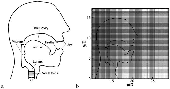
a) Human vocal tract system. b) Grid for voiced sound computation (only every 4th grid is plotted)
| (27) |
where l is the length of the duct, c is the speed of sound, and n = 1,2,3,…. In reality, these resonance frequencies are shifted by the cross-sectional area variation along the vocal tract, the radiation impedance at the mouth (open-end), and other coupling effects. The resulting resonance frequencies of the vocal-tract constitute the formant frequencies of voiced sound[1]. Therefore, the shape of vocal tract has a significant effect on the actual voiced sound generation. There have been several CAA studies on the human phonation problem[55, 56, 57]. All of these studies focused on the vocal fold vibration and laryngeal flow, and the vocal tract is assumed as a simple, infinitely long duct. In the present study, we directly compute the voiced sound generation for a given time-dependent glottal flow rate and also consider the propagation of this sound into the ambient region outside the speaker's mouth. In this preliminary study, two-dimensional computations are performed with geometries of human head and vocal tract representing the saggital symmetry plane as shown in Fig. 16a. Although the geometry has been simplified significantly, it is complex enough so as to pose a serious challenge to any conventional CAA method.
The computational grid around the head geometry is shown in Fig. 16b. The diameter of the trachea in the larynx D (see Fig. 16a) which is chosen as the characteristics length scale for this problem, and the outer domain boundaries are extended to 100D. A Cartesian grid with total 1024 × 1024 grid points is used and the head region is resolved by 600 × 800 grid points with uniform grid spacing, Δx = 0.02D. The vocal tract is modeled from the end of vocal folds and a glottal flow rate is prescribed as an inflow velocity boundary condition at the lower end of the vocal tract which coincides with the glottal outlet. The glottal gap size is assumed as d = 0.1D and velocity inlet boundary condition is only applied over this glottal gap in order to model the glottal. A parabolic profile is used for the velocity distribution and the maximum jet velocity, Vmax is chosen for the velocity scale. The dimensional values of length and velocity scale are D = 0.02(m) and Vmax = 34(m/s) [58]. Thus, the flow Mach number based on a maximum jet velocity is M = Vmax/c = 0.1.
In this study, the glottal flow rate waveform is modeled with the LF (Liljencrants-Fant) model[59] wherein the time derivative of the glottal flow rate, E = dQ/dt over one cycle is given by
| (28) |
where Eo = −Ee/{eαTe sin(ωoTe)}, E1 = Ee/(1 − e−β(Tc−Te)), T0 is a period, Te is the minimum flow rate derivative time, and Tc is a vocal fold close time, α, β, ωo, and Ee are parameters and E(t) satisfies the constraint: . The waveform for modal voice sound is constructed with the following parameters: α = 8.0, β = 20.0, ωo = 5.9631617, Ee = 0.8, and Te and Tc are set to 0.6T0 and 0.9T0, respectively. Figure 17a and 17b show the flow rate wave form (Q) and its time derivative (E). The fundamental frequency, f0 = 1/T0 is set to 125(Hz) which is a typical value of the adult male voice.
Figure 17.

a) Glottal flow rate wave form (Q) and b) its time derivative (E = dQ/dt) made with the LF model, Eq.(28).
The flow field is computed with the immersed boundary solver of Mittal et al.[33] for about 40 glottal cycles (40T0). With the fluctuating inlet flow rate, a pulsatile jet flow is developed at the vocal tract inlet and the instantaneous vorticity field is shown in Fig. 18a. The shear layer of the pulsatile glottal jet rolls-up into vorticies, which interact with the boundaries and pair with the vortices formed in previous cycles. The vortices are eventually found to dissipate further downstream. The hydrodynamic pressure fluctuation monitored near the vocal tract inlet is plotted in Fig. 18b. The overall waveform of the hydrodynamic pressure fluctuation is very similar to the time derivative of glottal flow rate. This is to be expected since if one assumes the vocal tract system to be a quasi one-dimensional tube, the hydrodynamic pressure gradient along the vocal tract can be represented by
Figure 18.
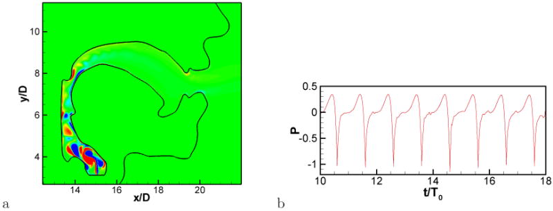
a) Instantaneous vorticity field of pulsatile jet flow in the vocal tract. b) Hydrodynamic pressure fluctuation monitored near the vocal tract inlet. Pressure is non-dimensionalized by .
| (29) |
where s is the distance variable along the vocal tract, and A is the cross-sectional area of the vocal tract. Equation (29) can be obtained by integrating the quasi one-dimensional momentum equation while neglecting the viscous effects and assuming the rate of cross-sectional area change is small. The small fluctuations observed in Fig. 18b are the effects of vortex motions. Since the hydrodynamic pressure fluctuation in the vocal tract will be the major source of sound generation and the pressure fluctuation is directly related with the time derivative of glottal flow rate as shown above, it is clear that the time derivative of glottal flow rate is primarily responsible for the voiced sound source mechanism.
The acoustic field computed with LPCE is shown in Fig. 19. One can see the generation of monopoles sound at the end of mouth and its propagation into the surrounding region. The acoustic wave-length corresponding to the fundamental frequency, f0 is about 136D, but a higher frequency component with a wavelengths of about 50D is also clearly visible. The time history of the acoustic pressure fluctuation monitored at 30D (about 60 cm) from the end of mouth and its sound pressure level (SPL) spectrum are shown in Fig. 20. The acoustic waveform is quite different from the hydrodynamic pressure fluctuation and its spectral peak is observed at the third harmonic of the fundamental frequency. As mentioned above, this is due to the resonance effect of the vocal tract system. The length of current vocal tract system is about l = 12.5D and this results in the first resonance frequency based on Eq. (27) of F1 = 2.72f0 (about 340Hz). Although the observed resonance frequency is slightly shifted from this value, the estimated F1 is near the third harmonic of the fundamental frequency and also explains the amplification of higher frequency components. In the ‘source-filter mechanism’ widely used in the analysis of voiced sound studies [1], the voiced sound signal is related to the glottal source (glottal flow rate or its time derivative) using a filter or transfer function which represents the acoustic response of the vocal tract. This transfer function can be computed with the present results. In the frequency domain, the transfer function (TF) can be estimated as
Figure 19.
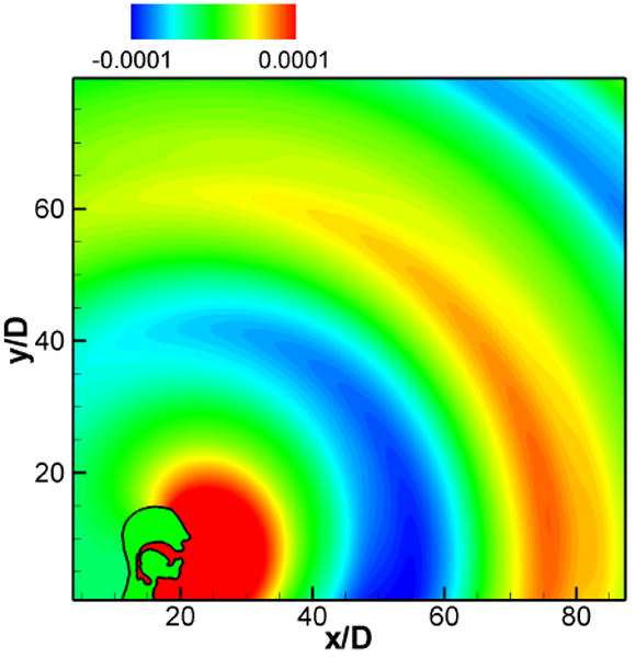
Instantaneous acoustic field, total pressure fluctuation, Δp′ contours, non-dimensionalized by ρ0c2.
Figure 20.

a) Time history of fluctuating pressure monitored at 30D from the end of mouth. Pressure fluctuation is non-dimensionalized by ρ0c2. b) Solid: sound pressure level (SPL) spectrum at 30D from the end of mouth. Dash-dot line: Envelope of the spectrum of E = dQ/dt shown in Fig. 17b.
| (30) |
where E is the time rate of change of the glottal flow rate. The spectrum of time derivative of glottal flow rate, E is plotted along with the SPL spectrum of acoustic signal at 30D from the end of mouth in Fig. 20b. The transfer function is computed by Eq. (30) at every harmonic of the fundamental frequency, f = nf0 and plotted in Fig. 21. The transfer function represents the acoustic response of the vocal tract system and one can clearly see the formant frequencies[1] of the current vocal tract system. The first formant corresponding to 350 Hz is close to the F1 value estimated with Eq. (27), but higher formant frequencies (683, 1554, 2093) are significantly shifted from the Fn values. The advantage of this direct computation of transfer function is that all the effects such as area variation, radiation impedance, and acoustic energy dissipation can be resolved without assumption or modeling. Moreover, the effect of the base flow can also be included in order to extract the finer features of the voiced sound. The directly computed transfer function would be quite helpful in the study of glottal source by the inverse filtering of voice sound signal[60].
Figure 21.

Transfer function computed by Eq. (30). The values are computed at the each harmonics of fundamental frequency and the continuous curve is made by parametric Splines.
Although the present voiced sound computations are performed with two-dimensional geometries, the fundamental mechanisms of voice sound generation are well resolved. In future work, we will consider actual three-dimensional geometry obtained with CT and ultrasound imaging [61] and also dynamic coupling with the vocal fold motion and laryngeal flow for the real voiced sound computation.
3.4. Flow-Noise from a Modeled Air-Conditioning Vent
The flow-induced noise by the deflector grille of the air-conditioning vent is known as one of the major interior noise components for automobile[62]. The sound generated by the grille is a complex problem whereas multiple deflectors result in a complex flow field and the generated sound also interacts with deflectors and the duct. In this section, the flow-induced noise produced by a deflector grille on an air conditioning vent is considered. This problem is considered here in order to demonstrate the capability of the present method for modeling complex low Mach number flow induced noise problems in engineering application.
The geometry and configuration of air conditioning vent and deflector grille considered in this study are shown in Fig. 22a. The deflectors are idealized by rounded plates and their length and thickness are l = 0.3D and h = 0.06D, respectively where D is the duct height and the deflector angle is set to 30 degrees. The relative dimensions of the duct and the deflectors are based on the Ref.[62]. A parabolic velocity profile is applied at the duct inlet and the maximum velocity Umax is chosen for the velocity scale. The Reynolds number and flow Mach number are set to ReD = UmaxD/ν = 10,000 and M = Umax/c = 0.1, respectively. The computational domain boundary is extended to 12D in x and y direction and open(velocity gradient zero)/radiation(ETA) boundary conditions are applied at these domains for flow and acoustic solver, respectively. The simulations employ a high-density non-uniform 1024 × 1024 Cartesian grid (shown in Fig. 22b) with a minimum grid spacing Δxmin = Δymin = 0.002D. The simulations are carried out on 256 processors of NICS-Kraken.
Figure 22.
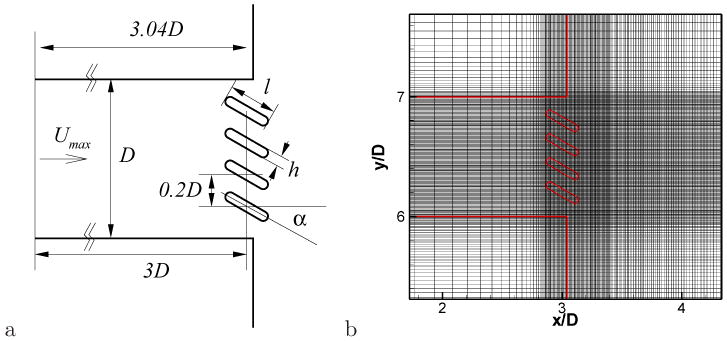
a) Modeling of air conditioning vent and deflector grille. b) Computational grid (every 4th grid is only plotted)
The flow field is computed with the incompressible flow solver and the instantaneous vorticity field is shown in Fig. 23a. The Reynolds number based on the deflector-plate thickness is 600 and therefore as expected, Karman vortex shedding is observed in the deflector wakes. For the uppermost deflector, a leading-edge separation vortex is also observed and all of these vortices interact in a highly complex manner in the grille wake. Figure 23b shows the vertical velocity (V) fluctuation monitored at the near wake of each deflector. The quasi-periodic velocity fluctuation caused by the Karman vortex shedding is clearly exhibited, especially for the lowest deflector (deflector 4). The Strouhal number for the vortex shedding of this deflector based on the deflector thickness is Sth = 0.27. For the uppermost deflector, the leading-edge separation affects the vortex shedding, and the dominant vortex shedding frequency for this deflector (deflector 1) is about 0.12. Vortex shedding from Deflector 2 is clearly affected significantly by the vortices from deflector 1.
Figure 23.
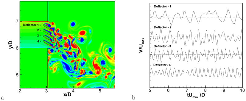
a) Instantaneous vorticity field around deflectors. b) vertical velocity component (V) fluctuations monitored at the near wake of each deflector.
The instantaneous acoustic field computed by LPCE is visualized in Fig. 24a with the dilatation rate, (∇ · u⃗′) field to show the structure more clearly. The power spectral densities of pressure fluctuation, Δp′, at four monitoring points (A-D) are also plotted in Fig. 24b. For the present low Mach number flow noise problem, the dipole sound generated by the vortex shedding for each deflector is expected to be the dominant noise source. The most clearly visible acoustic wave in Fig. 24a has acoustic wave length about 2D. Also, in Fig. 24b, the dominant peak is observed at Sth = 0.3, of which wave length is 2D. Since this peak frequency is very close to the Karman vortex shedding frequency, Sth = 0.27, it is conjectured that the Karman vortex shedding is the dominant source mechanism. However, it should be noted that the sound sources are located at the duct outlet, and the generated sound wave interact significantly with the duct. In a previous experimental study[62], it was found that the duct transversal mode plays an important role on the noise generated by the deflector grille. The observed dominant acoustic wave length of 2D (Sth = 0.3) also matches the wave length of duct transversal mode. Therefore, it is believed that the dominant radiated noise is a result of the coupling of vortex shedding at the deflectors and the duct transversal mode. A more detailed analysis for this problem will be performed in a future study which will include a more realistic 3D geometric model of the vent.
Figure 24.
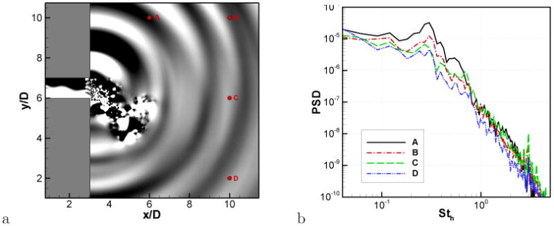
a) Instantaneous dilatation rate, (∇ · u⃗′) field. b) Power spectral densities of total pressure fluctuation monitored at points (A-D)
4. Conclusion
A sharp-interface, high-order immersed boundary method for the time-domain acoustic field computation is proposed. The sharp representation of immersed boundary interface by a ghost-point method and the boundary condition formulation using high-order polynomials enables accurate modeling of acoustic wave interaction with complex immersed boundaries. For the efficient computation of low Mach number flow noise, the proposed method is applied to the INS/LPCE hybrid method. Both the flow and acoustic solvers employ immersed boundary methods to resolve the flow and acoustic field around complex geometries respectively. The accuracy and fidelity of present method is demonstrated through verification against analytical solutions of canonical acoustic scattering problems as well as validation for the flow-induced noise by a flow past a circular cylinder. Two practical flow induced noise problems are also considered and the results show the potential of this new solver for addressing complex aeroacoustic sound generation problems.
Acknowledgments
The project described was supported by in part Grant Number ROIDC007125 from the National Institute on Deafness and Other Communication Disorders (NIDCD). The content is solely the responsibility of the authors and does not necessarily represent the official views of the NIDCD or the NIH. This research was also supported in part by the National Science Foundation through TeraGrid resources provided by the National Institute of Computational Science under grant number TG-CTS100002
References
- 1.Stevens KN. Acoustic Phonetics. The MIT Press; Cambridge, Massachusetts, London, England: 1998. [Google Scholar]
- 2.Mittal R, Simmons SP, Najjar F. Numerical Study of Pulsatile Flow in a Constricted Channel. J Fluid Mech. 2003;485:337–378. [Google Scholar]
- 3.El-Seaier M, Lilja O, Lukkarinen S, Sörnmo L, Sepponen R, Pesonen E. Computer-based Detection and Analysis of Heart Sound and Murmur. Annals of Biomedical Eng. 2005;33(7):937–942. doi: 10.1007/s10439-005-4053-3. [DOI] [PubMed] [Google Scholar]
- 4.Lehmann J. Auscultation of Heart Sounds. The American Journal of Nursing. 1972;72(7):1242–1246. [PubMed] [Google Scholar]
- 5.Howe MS. On the Hydroacoustics of a Trailing Edge with a Detached Flap. J Sound and Vibration. 2001;239(4):801–817. [Google Scholar]
- 6.Bourgoyne DA, Hamel JM, Judge CQ, Ceccio SL, Dowling DR. Hydrofoil near-wake Sound Sources at High Reynolds number. J Acou Soc Am. 2002;111(5):2425–2425. [Google Scholar]
- 7.Howe MS. Sound Produced by a Vortex Interacting with a Cavitated Wake. J Fluid Mech. 2005;543:333–347. [Google Scholar]
- 8.Terai T. On Calculation of Sound Fields around Three Dimensional Objects by Integral Equation Methods. J Sound Vib. 1980;69(1):71–100. [Google Scholar]
- 9.Shen L, Liu YJ. An adaptive fast multipole boundary element method for three-dimensional acoustic wave problems based on the Burton-Miller formulation. Comput Mech. 2007;40:461–472. [Google Scholar]
- 10.Colonius T, Lele SK. Computational aeroacoustics: progress on nonlinear problems of sound generation. Progress in Aerospace Sciences. 2004;40(6):345–416. [Google Scholar]
- 11.Bailly C, Bogey C, Marsden O. Progress in direct noise computation. International Journal of Aeroacoustics. 2010;9:123–143. [Google Scholar]
- 12.Lele SK. Compact Finite Difference Schemes with Spectral-like Resolution. J Comput Phys. 1992;103:16–42. [Google Scholar]
- 13.Tam CKW, Webb JC. Dispersion-Relation-Preserving Finite Difference Schemes for Computational Acoustics. J Comput Phys. 1993;107:262–281. [Google Scholar]
- 14.Sherer SE, Scott JN. High-order Compact Finite Difference methods on General Overset Grids. J Comput Phys. 2005;210:459–496. [Google Scholar]
- 15.Sherer SE, Visbal MR. High-order Overset-grid Simulations of Acoustic Scattering from Multiple Cylinders, Proc. of the Fourth Computational Aeroacoustics (CAA) Workshop on Benchmark Problems, NASA/CP-2004-212954. 2004:255–266. [Google Scholar]
- 16.Hu FQ, Hussaini MY, Rasetarinera P. An Analysis of the Discontinuous Galerkin for Wave Propagation Problems. J Comput Phys. 1999;151:921–946. [Google Scholar]
- 17.Chevaugeon N, Hillewaert K, Gallez X, Ploumhans P, Remacle JF. Optimal Numerical Parameterization of Discontinuous Galerkin Method applied to Wave Propagation Problems. J Comput Phys. 2007;223:188–207. [Google Scholar]
- 18.Dumbser M, Munz CD. ADER Discontinuous Galerkin Schemes for Aeroacoustics. CRMecanique. 2005;333:683–687. [Google Scholar]
- 19.Toulorge T, Reymen Y, Desmet W. A 2D Discontinuous Galerkin Method for Aeroacoustics with Curved Boundary Treatment. Proc. of International Conference on Noise and Vibration Engineering (ISMA2008); 2008; pp. 565–578. [Google Scholar]
- 20.Mittal R, Iaccarino G. Immersed Boundary Methods. Annu Rev Fluid Mech. 2005;37:239–261. [Google Scholar]
- 21.Casalino D, Di Francescantonio P, Druon Y. GFD Predictions of Fan Noise Propagation. AIAA Paper, 2004-2989; 2004. [Google Scholar]
- 22.Arina R, Mohammadi B. An Immersed Boundary Method for Aeroacoustics Problems. AIAA Paper, 2008-3003; 2008. [Google Scholar]
- 23.Cand M. 3-Dimensional Noise Propagation using a Cartesian Grid. AIAA Paper, 2004-2816; 2004. [Google Scholar]
- 24.Liu M, Wu K. Aerodynamic Noise Propagation Simulation using Immersed Boundary Method and Finite Volume Optimized Prefactored Compact Scheme. J Therm Sci. 2008;17(4):361–367. [Google Scholar]
- 25.Linnick MN, Fasel HF. A high-order immersed interface method for simulating unsteady incompressible flows on irregular domains. J Comput Phys. 2005;204:157–192. [Google Scholar]
- 26.de Tullio MD, De Palma P, Iaccarino G, Pascazio G, Napolitano M. An Immersed Boundary Method for Compressible Flows using Local Grid Refinement. J Comput Phys. 2007;225:2098–2117. [Google Scholar]
- 27.De Palma P, de Tullio MD, Pascazio G, Napolitano M. An Immersed Boundary Method for Compressible Viscous Flows. Comput & Fluids. 2006;35:693–702. [Google Scholar]
- 28.Ghias R, Mittal R, Dong H. A Sharp Interface Immersed Boundary Method for Compressible Viscous Flows. J Comput Phys. 2007;225:528–553. [Google Scholar]
- 29.Liu Q, Vasilyev OV. A Brinkman Penalization Method for Compressible Flows in Complex Geometries. J Comput Phys. 2007;227:946–966. [Google Scholar]
- 30.Hardin JC, Pope DS. An Acoustic/Viscous Splitting Technique for Computational Aeroacoustics. Theoret Comput Fluid Dynamics. 1994;6:323–340. [Google Scholar]
- 31.Seo JH, Moon YJ. The Perturbed Compressible Equations for Aeroacoustic Noise Prediction at Low Mach Numbers. AIAA Journal. 2005;43:1716–1724. [Google Scholar]
- 32.Seo JH, Moon YJ. Linearized Perturbed Compressible Equations for Low Mach Number Aeroacoustics. J Comput Phys. 2006;218:702–719. [Google Scholar]
- 33.Mittal R, Dong H, Bozkurttas M, Najjar FM, Vargas A, von Loebbecke A. A Versatile Sharp Interface Immersed Boundary Method for Incompressible Flows with Complex Boundaries. J Comput Phys. 2008;227:4825–2852. doi: 10.1016/j.jcp.2008.01.028. [DOI] [PMC free article] [PubMed] [Google Scholar]
- 34.Luo H, Mittal R, Zheng X, Bielamowicz SA, Walsh RJ, Hahn JK. An Immersed-Boundary Method for Flow-Structure Interaction in Biological Systems with Application to Phonation. J Comput Phys. 2008;227:9303–9332. doi: 10.1016/j.jcp.2008.05.001. [DOI] [PMC free article] [PubMed] [Google Scholar]
- 35.Lighthill MJ. On Sound Generated Aerodynamically. I. General Theory. Proc of Royal Society of London, Ser A. 1952;211:564–587. [Google Scholar]
- 36.Seo JH, Moon YJ. Aerodynamic Noise Prediction for Long-span Bodies. J Sound and Vibration. 2007;306:564–579. [Google Scholar]
- 37.Moon YJ, Seo JH, Bae YM, Roger M, Becker S. A hybrid prediction for low-subsonic turbulent flow noise. Computers & Fluids. 2010;39:1125–1135. [Google Scholar]
- 38.Goldstein ME. A Generalized Acoustic Analogy. J Fluid Mech. 2004;488 [Google Scholar]
- 39.Chorin AJ. On the Convergence of Discrete Approximations to the Navier-Stokes Equations. Math Comput. 1969;23(106):341–353. [Google Scholar]
- 40.Jameson A. Numerical solution of the Euler equations for compressible inviscid fluds. In: Angrand F, Dervieux A, De side ri JA, Glowinski R, editors. Numerical Methods for the Euler Equations of Fluid Dynamics. SIAM; Philadelphia: 1985. pp. 199–245. [Google Scholar]
- 41.Gaitonde D, Shang JS, Young JL. Practical Aspects of Higher-order Accurate Finite Volume Schemes for Wave Propagation Phenomena. Int J Numer Method in Eng. 1999;45:1849–1869. [Google Scholar]
- 42.Visbal MR, Gaitonde DV. High-order accurate methods for complex unsteady subsonic flows. AIAA J. 1999;37(10):1231–1239. [Google Scholar]
- 43.Carnahan B, Luther HA, James OW. Applied Numerical Methods. Wiley; New York: 1969. [Google Scholar]
- 44.Li Z. A fast interactive algorithm for elliptic interface problems. SIAM J Numer Anal. 1998;35(1):230–254. [Google Scholar]
- 45.Press WH, Teukolsky SA, Vetterling WT, Flannery BP. Numerical Recipes: The art of scientific computing. Third. Cambridge Univ. Press; Cambridge, New York, Melbourne, Madrid, Cape Town, Singapore, Sao paulo: 2007. [Google Scholar]
- 46.Gaitonde DV, Visbal MR. Technical Paper 99-0557. AIAA Press; Washington, DC: 1999. Further Development of a Navier-Stokes Solution Procedure Based on Higher-Order Formulations. [Google Scholar]
- 47.Visbal MR, Gaitonde DV. On the Use of Higher-Order Finite-Difference Schemes on Curvilinear and Deforming Meshes. J Comput Phys. 2002;181:155–185. [Google Scholar]
- 48.Edgar NB, Visbal MR. A General Buffer Zone Type Non-reflecting Boundary Condition for Computational Aeroacoustics. AIAA paper 2003-3300; 2003. [Google Scholar]
- 49.Tam CKW, Hardin JC, editors. NASA-CP-3352. 1997. Second Computational Aeroacoustics (CAA) Workshop on Benchmark Problems. [Google Scholar]
- 50.Sherer SE. Scattering of sound from axisymetric sources by multiple circular cylinders. J Acoust Soc Am. 2004;115:488–496. doi: 10.1121/1.1641790. [DOI] [PubMed] [Google Scholar]
- 51.Morris PJ. Scattering of Sound from a Spatially Distributed, Spherically Symmetric Source by a Sphere. J Acoust Soc Am. 1995;98:3536–3539. [Google Scholar]
- 52.Williamson CHK. Vortex Dynamics in the Cylinder Wake. Annu Rev Fluid Mech. 1996;28:477–539. [Google Scholar]
- 53.Henderson RD. Detail of the Drag Curve near the Onset of Vortex Shedding. Phys of Fluids. 1995;7:2102–2104. [Google Scholar]
- 54.Titze IR. Principles of Voice Production. Prentice Hall; 1994. [Google Scholar]
- 55.Zhao W, Zhang C, Frankel SH, Mongeau L. Computational Aeroacoustics of Phonation, Part I: Computational Methods and Sound Generation Mechanism. J Acou Soc of America. 2002;112:2134–2146. doi: 10.1121/1.1506693. [DOI] [PubMed] [Google Scholar]
- 56.Bae Y, Moon YJ. Computation of Phonation Aeroacoustics by an INS/PCE Splitting Method. Comput & Fluids. 2008;37:1332–1343. [Google Scholar]
- 57.Link G, Kaltenbacher M, Breuer M, Dollinger M. A 2D Finite-element Scheme for Fluid-solid-acoustic Interaction and Its Application to Human Phonation. Comput Methods in Applied Mech Eng. 2009;198:3321–3334. [Google Scholar]
- 58.Zheng X, Bielamowicz S, Luo H, Mittal R. A Computational Study of the Effect of False Vocal Folds on Glottal Flow and Vocal Fold Vibration During Phonation. Annals of Biomedical Eng. 2009;37:625–642. doi: 10.1007/s10439-008-9630-9. [DOI] [PMC free article] [PubMed] [Google Scholar]
- 59.Fant G. Glottal Flow: Models and Interaction. J Phonet. 1986;14:393–399. [Google Scholar]
- 60.Plumpe MD, Quatieri TF, Reynolds DA. Modeling of the Glottal Flow Derivative Waveform with Application to Speaker Identification. IEEE Tran Speech and Audio Proc. 1999;7(5):569–586. [Google Scholar]
- 61.Stone M. Imaging the tongue and vocal tract. J Disorder of Communication. 1991;26:11–23. doi: 10.3109/13682829109011990. [DOI] [PubMed] [Google Scholar]
- 62.Guerin S, Thomy E, Wright MCM. Aeroacoustics of automotive vents. J Sound Vib. 2005;285:859–875. [Google Scholar]