

Abstract
In this article, we present a new multiscale mathematical model for solid tumour growth which couples an improved model of tumour invasion with a model of tumour-induced angiogenesis. We perform nonlinear simulations of the multi-scale model that demonstrate the importance of the coupling between the development and remodeling of the vascular network, the blood flow through the network and the tumour progression. Consistent with clinical observations, the hydrostatic stress generated by tumour cell proliferation shuts down large portions of the vascular network dramatically affecting the flow, the subsequent network remodeling, the delivery of nutrients to the tumour and the subsequent tumour progression. In addition, extracellular matrix degradation by tumour cells is seen to have a dramatic affect on both the development of the vascular network and the growth response of the tumour. In particular, the newly developing vessels tend to encapsulate, rather than penetrate, the tumour and are thus less effective in delivering nutrients.
Keywords: Solid tumour, Avascular growth, Angiogenesis, Vascular growth, Multiscale mathematical model
1 Introduction
Cancer growth, and as a particular example in this paper, solid tumour growth, is a complicated phenomenon involving many inter-related processes across a wide range of spatial and temporal scales, and as such presents the mathematical modeller with a correspondingly complex set of problems to solve. The aim of this paper is to formulate a multi-scale mathematical model of solid tumour growth, incorporating three key features: the avascular growth phase, the recruitment of new blood vessels by the tumour (angiogenesis) and the vascular growth and host tissue invasion phase.
Solid tumours are known to progress through two distinct phases of growth—the avascular phase and the vascular phase. The initial avascular growth phase can be studied in the laboratory by culturing cancer cells in the form of 3D multicell spheroids. It is well known that these spheroids, whether grown from established tumour cell lines or actual in vivo tumour specimens, possess growth kinetics which are very similar to in vivo solid tumours. Typically, these avascular nodules grow to a few millimetres in diameter. Cells towards the centre, being deprived of vital nutrients, die and give rise to a necrotic core. Proliferating cells can be found in the outer cell layers. Lying between these two regions is a layer of quiescent (or hypoxic) cells, a proportion of which can be recruited into the outer layer of proliferating cells. Much experimental data has been gathered on the internal architecture of spheroids, and studies regarding the distribution of vital nutrients (e.g. oxygen) and metabolites within the spheroids have been carried out. See, for example, the recent reviews by Walles et al. [69], Kim [37], Kunz-Schughart et al. [39], Chomyak and Sidorenko [19] and the references therein.
The transition from the relatively harmless and confined dormant avascular state to the vascular state, wherein the tumour possesses the ability to invade surrounding tissue and metastasise to distant parts of the body, depends upon the ability of the tumour to induce new blood vessels from the surrounding tissue to sprout towards and then gradually surround and penetrate the tumour, thus providing it with an adequate blood supply and microcirculation. Tumour-induced angiogenesis, the process by which new blood vessels develop from an existing vasculature, through endothelial cell sprouting, proliferation and fusion, is therefore a crucial part of solid tumour growth. Sustained angiogenesis is a hallmark of cancer [33]. Mature endothelial cells are normally quiescent and, apart from certain developmental processes (e.g. embryogenesis and wound healing), angiogenesis is generally a pathological process implicated in arthritis, some eye diseases and solid tumour development, invasion and metastasis. Tumour-induced angiogenesis is believed to start when a small avascular tumour exceeds a critical diameter (∼2 mm), above which normal tissue vasculature is no longer able to support its growth. At this stage, the tumour cells lacking nutrients and oxygen become hypoxic. In response, the tumour cells secrete a number of diffusible chemical substances—tumour angiogenic factors (TAF)—into the surrounding tissues and extracellular matrix (ECM). The TAF diffuses into the surrounding tissue and eventually reach the endothelial cells (EC) that line nearby blood vessels. ECs subsequently respond to the TAF concentration gradient by degrading the basement membrane surrounding the parent vessel, forming sprouts, proliferating and migrating towards the tumour. It takes approximately 10–21 days for the growing network to link the tumour to the parent vessel, and this vascular connection subsequently provides all the nutrients and oxygen required for continued tumour growth. An excellent summary of all the key cell-biological processes involved in angiogenesis can be found in the comprehensive review articles of Paweletz and Knierim [54] and Carmeliet [16]. Once vascularized the solid tumours grow rapidly as exophytic masses. In certain types of cancer, e.g. carcinoma arising within an organ, this process typically consists of columns of cells projecting from the central mass of cells and extending into the surrounding tissue area. The local spread of these carcinoma often assume an irregular jagged shape. By the time a tumour has grown to a size whereby it can be detected by clinical means, there is a strong likelihood that it has already reached the vascular growth phase.
Cancers also possess the ability to actively invade the local tissue and then spread throughout the body. Invasion and metastasis are the most insidious and life-threatening aspects of cancer [43,44]. Indeed, the prognosis of a cancer is primarily dependent on its ability to invade and metastasize. Many steps that occur during tumour invasion and metastasis require the regulated turnover of extracellular matrix (ECM) macromolecules, catalyzed by proteolytic enzymes released from the invading tumour. Proteases give cancers their defining characteristic—the ability of malignant cells to break out of tissue compartments. Motility, coupled with regulated, intermittent adhesion to the extracellular matrix and degradation of matrix molecules, allows an invading cell to move through the extracellular matrix [28,40,44].
The most significant turning point in cancer, however, is the establishment of metastasis. The metastatic spread of tumour cells is the predominant cause of cancer deaths, and with few exceptions, all cancers can metastasize. Metastasis is defined as the formation of secondary tumour foci at a site discontinuous from the primary tumour [43,44]. Metastasis unequivocally signifies that a tumour is malignant and this is in fact what makes cancer so lethal. In principal, metastases can form following invasion and penetration into adjacent tissues followed by dissemination of cells in the blood vascular system (hematogeneous metastasis) and lymphatics (lymphatic metastases).
Since the seminal work of Greenspan [32] the mathematical modeling of avascular solid tumour growth, like its subject, has been rapidly expanding. Most models in this area consist of systems of nonlinear partial differential equations (e.g. see [13–15]), and may be described as macroscopic. The review paper of Araujo and McElwain [6] provides an excellent overview. See also the recent reviews by Quaranta et al. [62], Byrne et al. [12], Sanga et al. [64], Graziano and Preziosi [31] and Roose et al. [63]. Likewise, modeling tumour-induced angiogenesis has a well-established history beginning with the work of Balding and McElwain [9]. The review papers of Mantzaris et al. [49] and Chaplain et al. [18] provide an excellent overview of the work in this area. However, unlike avascular growth and angiogenesis, vascular tumour growth has received considerably less attention in the mathematical modeling literature. See [17,52] for early work on vascular tumour growth and invasion.
Recently, Zheng et al. [71] developed and coupled a level-set method for solid tumour growth with a hybrid continuous–discrete model of angiogenesis originally developed by Anderson and Chaplain [4]. This work served as a building block for studies of chemotherapy [65] and morphological instability and tumour invasion [20, 27]. Hogea et al. [34] have also begun to investigate tumour induced angiogenesis and vascular growth using a level-set method coupled with a continuous model of angiogenesis. Following the strategy pioneered by Zheng et al. [71], Frieboes et al. [26] coupled a mixture model with a lattice-free continuous–discrete model of angiogenesis (originally developed by Planck and Sleeman [55]) and studied vascular tumour growth in three dimensions. In these works, however, the effects of blood flow through and subsequent remodeling of the vascular network were not included. Recently, the effects of blood flow through a vascular network on tumour growth were considered by Alarcón et al. [1], Lee et al. [41], Bartha and Rieger [10], Welter et al. [70] using cellular automaton (CA) tumour growth models coupled with network models for the vasculature. These authors investigated vascular network inhomogeneities, the stress-induced collapse of blood vessels and the implications for therapy. Because of the computational cost of simulating cell growth using CA, these studies are limited to small scales.
In this paper, we couple an improved continuum model of solid tumour invasion (following [48]) that is capable of spanning the 102 μm-cm scale and accounts for cell–cell, cell–ECM adhesion, ECM degradation, and tumour cell migration, proliferation, and necrosis with a model of tumour-induced angiogenesis (following [50]) that accounts for blood flow through the vascular network, non-Newtonian effects and vascular network remodeling, due to wall shear stress and mechanical stresses generated by the growing tumour, to produce a new multi-scale model of vascular solid tumour growth. As in [71], the invasion and angiogenesis models are coupled through the tumour angiogenic factors (TAF), that are released by the tumour cells, and through the nutrient extravasated from the neo-vascular network. As the blood flows through the neo-vascular network, nutrients (e.g. oxygen) are extravasated and diffuse through the ECM triggering further growth of the tumour, which in turn influences the TAF expression. In addition, the extravasation is mediated by the hydrostatic stress generated by the growing tumour and, as mentioned above, the hydrostatic stress also affects vascular remodeling by restricting the radii of the vessels. The vascular network and tumour progression are also coupled via the ECM as both the tumour cells and the ECs upregulate matrix degrading proteolytic enzymes which cause localized degradation of the ECM which in turn affects haptotactic migration.
We perform simulations of the multi-scale model that demonstrate the importance, on tumour invasion of the host tissue, of the nonlinear coupling between the growth and remodeling of the vascular network, the blood flow through the network and the tumour progression. Consistent with clinical observations, the hydrostatic stress generated by tumour cell proliferation shuts down large portions of the vascular network dramatically affecting the flow, the subsequent network remodeling, the delivery of nutrients to the tumour and the subsequent tumour progression. In addition, ECM degradation by tumour cells is seen to have a dramatic affect on both the development of the vascular network and the growth response of the tumour. In particular, when the ECM degradation is significant, the newly formed vessels tend to encapsulate, rather than penetrate, the tumour and are thus less effective in delivering nutrients.
The outline of the paper is as follows. In Sect. 2, we present the mathematical models, and we briefly describe the numerical techniques in Sect. 3. In Sect. 4, we present numerical results, and future work is discussed in Sect. 5. Details of the mathematical modeling and numerical methods are presented in the supplementary materials.
2 The mathematical model
Here, we present the non-dimensional model, starting first with the model of tumour invasion in Sect. 2.1 and followed by the model of tumour-induced angiogenesis in Sect. 2.2. Here, time is non-dimensionalized by the characteristic tumour cell proliferation time (i.e., 1/λm where λm ≈ 2/3 day−1 is the mitosis rate) and space is non-dimensionalized by the characteristic diffusion penetration length (i.e., , where and are characteristic values of the oxygen diffusion coefficient and uptake rate in the proliferating tumour region, respectively). The non-dimensionalization of the parameters and the corresponding values used in the numerical simulations are presented in the supplementary materials.
2.1 The tumour invasion model
To accurately model tumour growth in heterogeneous tissues, we develop a mathematical model that accounts for spatially dependent cell necrosis, cell apoptosis, cell–cell and cell–matrix adhesion, matrix degradation, cell proliferation and cell migration. The model is based on continuum reaction–diffusion equations that describe these processes and is a generalization and improvement of earlier models (see the reviews listed previously and recent work by Macklin and Lowengrub [45–48]). We present the model in 2D, but it is equally valid for the 3D case as well.
Let Ω denote a tumour mass, and let Σ denote its boundary. The tumour can be divided into three regions: a proliferating rim ΩP where the tumour cells have sufficient nutrient levels for proliferation; a hypoxic/quiescent region ΩH where the nutrient levels are too low for normal metabolic activity but not so low that the cells begin to die; and a necrotic region ΩN where the nutrient level has dropped so low that the tumour cells die and are degraded. Because necrosis is irreversible, we track the necrotic core and its interface ΣN separately of the tumour interface. See Fig. 1.
Fig. 1.

Schematic of the tumour regions. ΩP, ΩH and ΩN are the proliferating, quiescent/hypoxic and necrotic regions, respectively
2.1.1 Nutrient transport
We model the net effect of nutrients (e.g., oxygen and glucose) and growth-promoting and –inhibiting factors with a single nutrient σ. Here, we focus our attention on the role of oxygen which is supplied by the vascular network via the red blood cells. This can be modelled using the haematocrit which represents the volume fraction of red blood cells contained in the blood. Oxygen and other nutrients are supplied by the preexisting bulk vasculature and the neo-vasculature at rates and , diffuses throughout the cancerous and non-cancerous tissue, is uptaken in the non-necrotic portions of the tumour, and decays elsewhere (see below). Wherever the oxygen level inside the tumour drops below a threshold value σH, the tumour cells become hypoxic (quiescent), cease proliferating and uptake nutrient at a lower rate. If the oxygen level falls further below a threshold value σN, then the tumour cells become necrotic. Inside the necrotic core, oxygen reacts with cellular debris to form reactive oxygen species [29,38], which we model by a decay term. Since oxygen diffusion occurs more rapidly than cell-mitosis (the time scale on which the equations are non-dimensionalized), these processes are described by the quasi-steady reaction diffusion equation
| (1) |
where D is the diffusion coefficient, the parameter λσ combines the effects of oxygen uptake and decay and takes the form
| (2) |
where pσ and qσ are smooth interpolating functions (the precise forms are given in the supplementary materials) and E0 is the density of the original ECM which is used to assess changes in uptake/decay in the host microenvironment (see Sect. 2.1.3). The interpolating function qσ satisfies , where σH and σN are the oxygen concentration thresholds for quiescence and necrosis, respectively and λ̄H is the rate of oxygen uptake by quiescent cells in the hypoxic tumour. Further, λ̄tissue and λ̄σ are the rates of oxygen uptake in the host microenvironment and in the proliferating tumour regions respectively, and λ̄N is the rate of oxygen decay in the necrotic portion of the tumour. We note that because the location of the viable, hypoxic, and necrotic tumour regions depends upon the oxygen concentration σ, the uptake/decay term λσ introduces nonlinearity.
The two remaining terms and in Eq. 1 reflect the oxygen-tissue transfer from the pre-existing and neo-vascular blood vessels respectively, and are given by:
| (3) |
and
| (4) |
where and are constant transfer rates from the pre-existing and neo-vascular vessels. Here, Bpre is the (non-dimensional) blood vessel density of the pre-existing vessels whose locations are assumed to be unchanging in time. In fact, we take a uniform distribution of pre-existing vessels in the host tissue and Bpre satisfies Eq. 19 below where MDE is assumed to degrade the pre-existing vasculature. The function Bneo (x, t) = 1neo is the characteristic or indicator function of the neo-vasculature (i.e., equal to 1 at the locations of the new vessels), and 1Ω is the characteristic function of the tumour region Ω (i.e., equal to 1 inside the tumour and 0 in the tumour exterior). Further, P is the oncotic (solid/mechanical/hydrostatic) pressure, Pvessel and h are the dimensional pressure and the haematocrit in the neo-vascular network, respectively. The constants H̄D and h̄min reflect the normal value of haematocrit in the blood (generally about 0.45) and the minimum haematocrit needed to extravasate oxygen, respectively. The haematocrit is modelled via the blood flow in the vascular network and is determined from the angiogenesis model. This provides one aspect of the coupling between the tumour growth and angiogenesis models. A second mode of coupling between the two models occurs through the cutoff function c (Pvessel, P) which is given by:
| (5) |
where pcutoff is a cubic, interpolating polynomial given in the supplementary materials. Namely, large oncotic pressures may prevent extravasation and transfer of oxygen from the vessels into the tissue. Later, we will discuss how the oncotic pressure may also constrict the neovessels. Further, in Eq. 5,
| (6) |
where P̄vessel is a characteristic pressure scale and P̄scale is a scale factor. Note that we could have analogously taken the oxygen transfer rate from the pre-existing vessels to also be coupled to the haematocrit and blood vessel pressure. This will be explored in a future work.
The oxygen source terms in Eqs. 3 and 4 are designed such that for sufficiently large transfer rates and , the oxygen concentration σ ≈ 1 the spatial locations of the pre-existing and neo- vessels. In practice, we will take large but small which models the supply of only a small amount of oxygen in the host tissue from pre-existing vessels. We will assume a parent vessel, located at the boundary of the computational microenvironment domain as discussed below, supplies the bulk of the oxygen in the host tissue. Note that oxygen flux conditions across the pre-existing and neo-vasculature could be imposed (e.g., see [1]).
The boundary conditions for Eq. 1 are taken to be a combination of Dirichlet and Neumann conditions. In particular, in the simulations we present below, we assume a parent vessel coincides the upper boundary of the computational domain and therefore we impose σ = 1 (a Dirichlet condition). Zero Neumann conditions, ∂σ/∂n = 0, are imposed along the other boundaries of the computational domain.
2.1.2 Tumour mechanics and the cell velocity
The tumour cells, the ECM and host (non-cancerous) cells are influenced by a combination of forces which contribute to the cellular velocity field. The proliferating cells generate an oncotic mechanical pressure (hydrostatic stress) that also exerts force on the ECM and host cells. The cells respond to pressure variations by overcoming cell–cell and cell–ECM adhesion and migrating through the microenvironment. The ECM may also deform, degrade and remodel in response to pressure and to enzymes released by the cells. The cells may respond haptotactically to adhesion gradients in the ECM.
Following previous work, we assume that all solid phases move with a single cellular velocity field and we model the cellular motion within the ECM as incompressible fluid flow in a porous medium. In the future, we plan to use mixture models (e.g., [2,7,8,11,21]) to relax these assumptions. In this simplified description of tumour mechanics used here, Darcy's law is taken as the constitutive assumption and thus the velocity is proportional to the forces in the problem. See [2] and [11] for a motivation of this approach from a mixture modeling perspective. Accordingly, the non-dimensional velocity is given by
| (7) |
where μ is the cell-mobility which models the net effects of cell–cell and cell–matrix adhesion, E is the ECM density (e.g. a non-diffusible matrix macromolecule such as fibronectin, collagen or laminin) and χE is the haptotaxis coefficient. Models for μ and χE are given in Sect. 2.1.3. Further assuming that the density of tumour cells is constant in the viable region, the growth of the tumour is then associated with the rate of volume change:
| (8) |
where λP is the non-dimensional net proliferation rate. This implies that the non-dimensional pressure satisfies:
| (9) |
We assume that in the proliferating region, cell-mitosis is proportional to the amount of nutrient present and that apoptosis may occur. Volume loss may occur in the necrotic core and there is no proliferation in either the host microenvironment or the hypoxic/quiescent regions. We therefore take
| (10) |
where A is the non-dimensional apoptosis rate (“pre-programmed” cell death); and GN is the non-dimensional rate of volume loss in the necrotic core as water is removed and cellular debris are degraded. Assuming a uniform cell–cell adhesion throughout the tumour, cell–cell adhesion can be incorporated as a surface-tension like jump boundary condition at the tumour–host interface Σ:
| (11) |
where G is a non-dimensional parameter that measures the aggressiveness of the tumour (the strength of cell proliferation relative to cell–cell adhesion) and κ is the mean curvature of the interface. At the necrotic boundary ΣN we assume P is continuous. We assume that no voids form and therefore we take
| (12) |
where n is the unit outward normal to Σ. For simplicity, we will also assume that [∇E · n] = 0. At necrotic boundary, we assume analogous conditions. The velocity of the tumour–host interface Σ is then given by:
| (13) |
and the velocity of the necrotic boundary ΣN is
| (14) |
where nN is the outward unit normal vector along ΣN. In the far-field at the boundaries of the computational domain, the pressure is assumed to satisfy zero Neumann boundary conditions ∂P/∂n = 0.
2.1.3 Tumour-microenvironment interaction
We model tumour microenvironment by introducing an extracellular matrix density E that represents the density of non-diffusible matrix macromolecules such as fibronectin, collagen, elastin and laminin, etc. In addition, as mentioned earlier, we keep track of the density E0 of the original ECM and the pre-existing blood vessel density Bpre to assess the level of oxygen uptake and supply, respectively, in the microenvironment.
The tumour interacts with the microenvironment by responding to the nutrients supplied by the pre-existing and the neo-vasculature (e.g. see Eq. 1), remodeling the ECM locally by secreting both MDE and ECM macromolecules and by a hetereogeneous response to pressure and ECM adhesion gradients through non-constant cell-mobility and haptotaxis coefficients. In order for tumours cells to migrate into the porous matrix, they must overcome cell-matrix adhesion. However, in experiments, a maximum migration speed is obtained that depends on the level of integrin expression (e.g. [24,53]) and correspondingly a non-monotonic dependence of cell migration velocity on integrin expression and adhesion gradients in the ECM has been predicted [23,24]. This has been explained by the fact that while some integrins are required for focal adhesion based migration, too much focal contact strength can retard the detachment of cell's trailing edge from the ECM. While we do not model integrin expression directly here, we take this effect into account by making the haptotaxis coefficient a non-monotone function of E:
| (15) |
where χ̄E, min is the non-dimensional haptotaxis in low/high-density ECM, pχ is a non-monotone interpolating function with a maximum χ̄E,max located at . See the supplementary materials for the precise form of pχ. Although the mobility μ may also be non-monotone, for simplicity, we take a monotone decreasing function of E here:
| (16) |
where pμ is a smooth interpolating function (see the supplementary materials for a precise form). In a future work, we will investigate non-monotonic cell mobilities μ. In addition, the mobility and chemotaxis parameters may also be functions of oxygen concentration σ as hypoxic conditions may result in upregulation of HIF-1α target genes that may result in decreased cell–cell adhesion, among other effects, and therefore enable cells to more easily migrate through and invade the tumour microenvironment (e.g., see [25,36,56]). These effects will also be explored in a forthcoming work.
In order to migrate through the ECM and invade the host tissue, tumour cells secrete matrix degrading proteolytic enzymes (MDE), e.g. matrix metalloproteases and urokinase plasminogen activators, which cause the degradation of the ECM, provide space for the cells, and enhance the attachment of the cells to ECM macromolecules enabling the cells to exert traction forces to propel themselves through the ECM. In addition, the tumour cells remodel the ECM by secreting insoluble matrix macromolecules and possibly reorienting them. We note that during the angiogenic response of the host vasculature, an analogous molecular cascade occurs as tumour angiogenesis factors (TAF) and ECM macromolecules (e.g. fibronectin, collagen, laminin) bind to specific membrane receptors on ECs and activate the cells' migratory machinery. This leads to a remodeling of ECM similar to that described above for tumour cells. Here, we will not consider the effect of orientational remodeling. We model the remaining processes as follows. For the MDE, we take
| (17) |
where M is the nondimensional MDE concentration, DM = D̄M is the diffusion coefficient (assumed to be constant), and are the non-dimensional rates of production of MDE by the viable tumour cells (ΩV = ΩP ∪ ΩH) and the sprout tip ECs, respectively. Further, is the rate of decay (it is assumed that MDE is not used up as a result of the interaction with the ECM (Quaranta, private communication)). Finally, 1sprout tips is the characteristic function of the sprout tips. In particular, 1 sprout tips = 1 in small circle centered at each sprout tip and tends to zero smoothly, and rapidly, outside these circles. Because the diffusion coefficient of MDE, DM, is much smaller than that for oxygen diffusion the full time-dependent diffusion equation is used [67]. In the far-field (boundary of the computational domain), we take the zero Neumann boundary conditions ∂M/∂n = 0.
The ECM density satifies:
| (18) |
where and are the non-dimensional rates of production of ECM by the viable tumour cells and sprout-tip ECs and is the non-dimensional rate of matrix degradation by the MDE.
Finally, the original ECM and the pre-existing blood vessel density are assumed to be degraded by the MDE:
| (19) |
where and are non-dimensional degradation rates.
2.1.4 Tumour angiogenic factors
When tumour cells become hypoxic/quiescent, they are assumed to secrete tumour angiogenic factors (TAF), which diffuse into the surrounding tissue and attract ECs. ECs respond to the TAF by binding with it, proliferating and chemotaxing up the TAF gradient. The diffusion coefficient of TAF is similar to that of oxygen and so we model the production, diffusion, decay, and binding of TAF by
| (20) |
where T is the non-dimensional TAF concentration, DT = D̄T is the diffusion coefficient (assumed to be constant) and , , and denote the non-dimensional production, natural decay and binding rates of TAF. In the far-field at the boundary of the computational domain, we also take zero Neumann boundary conditions ∂T/∂n = 0.
2.2 Angiogenesis model
We begin with a description, in Sect. 2.2.1, of an initial mathematical model for the growth of a hollow capillary network in the absence of any blood flow. This follows [4]. Then, following [50], we will add the effects of blood flow and vascular network remodeling in Sects. 2.2.2 and 2.2.3, respectively.
2.2.1 Basic network model
As described earlier, TAF and ECM macromolecules bind to specific membrane receptors on ECs and activate the cells' migratory machinery. The model of EC migration given below describes how capillary sprouts emerging from a parent vessel migrate towards a tumour, leading to the formation of a vascular network that supplies nutrients for continued development. (See the supplementary materials for a schematic diagram). At this level, since there is no flow or vessel remodeling, this model may perhaps be considered more appropriate at describing in vitro endothelial cell migration and capillary sprout formation. The model, inspired by the tumour angiogenesis model developed by Anderson and Chaplain [4], assumes that endothelial cells migrate through (i) random motility, (ii) chemotaxis in response to TAF released by the tumour and (iii) haptotaxis in response to ECM gradients. If we denote by n the non-dimensional endothelial cell density per unit area, then the non-dimensional equation describing EC conservation is given by
| (21) |
See [50] and the supplementary materials for the non-dimensionalization. The diffusion (random migration) coefficient is D = D̄ (assumed to be constant), and the chemotactic and haptotactic migration are characterised by the functions , which reflects the decrease in chemotactic sensitivity with increased TAF concentration and , where for simplicity we have taken the haptotactic migration parameter to be constant. In a future work, we will investigate the heterogeneous response of the ECs to the ECM as discussed earlier in Sect. 2.1.3. The coefficients D̄, and characterise the non-dimensional random, chemotactic and haptotactic cell migration, respectively.
The displacement of each individual EC, located at the tips of each growing sprout, is given by the discretised form of the EC mass conservation equation (21) on a regular Cartesian mesh. The migration of each cell is consequently determined by a set of coefficients (P0–P4) emerging from this equation, which relate to the likelihood of the cell remaining stationary, moving left, right, up or down. These coefficients incorporate the effects of random, chemotactic and haptotactic movement and depend upon the local chemical environment (ECM density and TAF concentration). Proliferation of the endothelial cells at the capillary tips and branching at capillary tips are implemented in the model at the discrete level. Tip branching depends on the TAF concentration at a given spatial location. (See the supplementary materials and [4] for details). Using the above model it is possible to generate “hollow” capillary networks which are structurally similar to those observed experimentally.
2.2.2 Modelling blood flow in the developing capillary network
Blood is a complex multiphase medium, composed of many different constituents, including: red blood cells (erythrocytes), white blood cells (leukocytes), and platelets involved in clotting cascades. These solid elements represent approximately 45% of the total blood composition—red cells are predominant—and are carried in the plasma, which constitutes the fluid phase. A measure of the solid phase is given by the blood haematocrit, which represents the volume fraction of red blood cells contained in the blood. The average human haematocrit has a value of around 0.45. Because of its multiphasic nature, blood does not behave as a continuum and the viscosity measured while flowing at different rates in microvessels is not constant. The direct measurement of blood viscosity in living microvessels is very difficult to achieve with any degree of accuracy. However, by comparing the flow distribution in a numerical network (generated by a mathematical model) with a similar experimental system, Pries et al. [60] obtained
where μplasma is the plasma viscosity, and μrel is the relative viscosity that accounts for the effects of the blood haematocrit and the radius of the vessel. The apparent blood viscosity generally increases with decreasing capillary radius, although the precise relationship is nonlinear since it is actually haematocrit-dependent. See the supplementary materials for the precise form of μrel.
In order to calculate the flow within the entire interconnected network of capillaries, it is first necessary to decide upon a local relationship between the pressure gradient vessel ΔP and flow rate Q̇ at the scale of a single capillary element of length L and radius R. Such a relationship in the case of a non-Newtonian fluid can be approximated by the following Poiseuille-like expression:
| (22) |
In order to determine the pressure (and flow rate) and in the vascular network of interconnected capillary elements having distributed radii, one simply conserves mass (or flow if the fluid is incompressible) at each junction where capillary elements meet. (See the supplementary materials for a schematic diagram.) Hence, for each node (i, j) the following expression can be written:
| (23) |
where the index k refers to adjacent nodes and N = 4 in a fully connected regular 2D grid as considered in this paper (or N = 6 in 3D). This procedure leads to a set of linear equations for the nodal pressures (Pvessel,i) which can be solved numerically using any of a number of different algorithms including successive over-relaxation (SOR). Once the nodal pressures are known, Eq. 22 can be used to calculate the flow in each capillary element in turn. A more complete discussion of the procedure can be found in McDougall et al. [51,66]. The evolution of haematocrit h in the vessels is also calculated using mass conservation once the flow is determined.
2.2.3 Capillary vessel adaptation and remodeling
Blood rheological properties and microvascular network remodeling are interrelated issues, as blood flow creates stresses on the vascular wall (shear stress, pressure, tensile stress) which lead to adaptation of the vascular diameters via either vasodilatation or constriction. In turn, blood rheology (viscosity, haematocrit, etc.) is affected by the new network architecture. Consequently, we should expect adaptive angiogenesis to be a highly dynamic process. We follow the work of Pries et al. [57,59–61] in incorporating vessel adaptation into our model. In particular, we consider a number of stimuli that affect the vessel diameters. We account for the influence of the wall shear stress (Swss), the intravascular pressure (Sp), a metabolic mechanism depending on the blood haematocrit (Sm), as well as the natural tendency for vessels to shrink (Ss). These stimuli form a basic set of requirements in order to obtain stable network structures with realistic distributions of vessels diameters and flow velocities. The theoretical model for vessel adaptation assumes that the change in a flowing vessel radius ΔR over a time step Δτ, where time is scaled by the rate of the response of the vessel to wall shear stress (kw), is proportional to both the global stimulus acting on the vessel and to the initial vessel radius R, i.e.
| (24) |
We refer the reader to the supplementary materials for the definitions of the stimuli and a brief discussion. More details may be found in [50].
After the radius of the vessel is updated according to Eq. 24, the effect of the oncotic mechanical pressure P, generated by the proliferating and invading tumour, on the vessel radius is then taken into account. The tendency of the oncotic pressure to shrink the vessel is modelled by the simple cutoff:
| (25) |
where c (P, Pvessel) is the cutoff function introduced earlier in Eq. 5 and Rmin is a threshold minimum radius. This provides another means of coupling tumour invasion (and mechanics) with the angiogenic response and the developing neo-vascular network. In particular, the solid/mechanical pressure may constrict and cut off vessels in the neovasculature. To prevent singularities in practice, the radius of the vessel is constrained to lie between 2.0 and 14 μm which is the size of the parent capillary.
Inclusion of the above mechanisms into our modeling framework now allows us to simulate dynamic remodeling of a flowing vasculature. This significant improvement in angiogenesis modeling, introduced by McDougall et al. [50], allows us to describe vascular growth in a far more realistic manner, with areas of the capillary network dilating and constricting in response to variations in perfusion-related stresses, stimuli and pressure mechanical forces exerted on the host microenvironment by the invading tumour. The final step in the development of the complete dynamic adaptive tumour-induced angiogenesis (DATIA) model is to couple the network flow modeling approach outlined in this Section to the “hollow capillary” model derived from the endothelial cell migration equations described earlier. This is achieved through the role of wall shear stress.
Wall shear stress is known to play a leading role in the growth and branching of capillary vessel networks [57,58]. In order to “bring the morphological and the physiological concepts together” [68], the cell migration and flow models are coupled by incorporating the mechanism of shear-dependent vessel branching in addition to sprout-tip branching via local TAF concentrations. This enables the capillary network structures to adapt dynamically through adjuvant vessel branching in areas of the network experiencing increased shear stresses following anastomosis elsewhere in the system. We note that because the shear stress is due to the blood flowing through the capillaries, vessel branching can only occur after some degree of anastomosis has taken place. Therefore, the early stages of angiogenesis are primarily characterised by branching at the capillary tips which depends only on the TAF concentration. The combined effects of the local wall shear stress and TAF concentration upon vessel branching probability have been implemented in the model as described in the supplementary materials.
3 Numerical schemes
3.1 Tumour invasion model
The tumour invasion model described in Sect. 2.1 consists of a coupled system of nonlinear, elliptic and parabolic (reaction–diffusion) differential equations that must be solved on a complex, moving domain where the motion of the tumour/host boundary depends on gradients of the solutions to these equations. Further, one of these solutions—the pressure—is discontinuous across the tumour/host interface where the discontinuity depends on the geometry (i.e. the curvature) of the interface which is an additional source of nonlinearity. Therefore, standard finite difference methods cannot be used to accurately solve the system. Instead, specialized methods that can accurately take into account discontinuities in solutions and complex domains must be used. Here, we use a ghost-cell/level-set method and adapt and extend the numerical techniques we recently developed to solve this system [45–48]. In this approach, the equations are discretized on a regular Cartesian mesh and the difference stencils near discontinuities are modified. We note that other alternatives exist (see the discussion in [48]), but an advantage of our approach is that it can be implemented in a dimension-by-dimension manner, making the extension to 3D straightforward, and our algorithm is simpler to implement than the alternative approaches.
In this approach, the interface is captured as the zero set of an auxiliary function (the level-set function) ϕ satisfying ϕ < 0 inside Ω, ϕ > 0 outside Ω, and ϕ = 0 on the tumour/host interface Σ. Typically ϕ is taken to be an approximation to the signed distance function, i.e. |∇ϕ| ≈ 1. See the supplementary materials for a schematic diagram. The interface normal and curvature can easily be calculated from ϕ. The interface ΣN separating viable tumour cells from the necrotic cells is also captured using additional level set function boundary ϕN that satisfies the same properties as ϕ, only with ΩN and ΣN in place of Ω and Σ.
Away from Σ, the elliptic/parabolic equations can be discretized using centered finite differences. However, near the interface, the difference stencils need to be modified to account for possible jumps in solutions and in their normal derivatives. To do this, ghost cells on either side of the interface are introduced and the variables are extrapolated across the interface to ensure that the difference stencil effectively does not include nodes on the other side of the interface. The resulting nonlinear system is solved using an iterative algorithm. These techniques are described in the supplementary materials. See also [48] for additional detail.
3.2 The dynamic tumour-induced angiogenesis model
For a fixed tumour geometry and TAF distribution, the tumour vasculature is first grown using the basic network model given in Sect. 2.2.1; capillary tips may branch or anastomose during this stage. Further, the Cartesian mesh for the tumour growth system coincides with that used for the neo-vascular network. After a certain period of time, referred to as the capillary growth duration time, the fluid flow is solved in the fixed neovascular network and then the network is dynamically remodelled, following the algorithm described in Sects. 2.2.2 and 2.2.3, respectively. During the simulation of the flow, a CFL condition is imposed on the time step: Δτ ≈ min (Vcap, Q̇cap) where Vcap and Q̇cap are the velocity and flow rate in a capillary element. The minimum is taken over the neo-vascular network. This ensures haematocrit remains conserved during the simulation (e.g., [51]). Then process of blood flow, followed by remodeling, is repeated for an amount of time referred to as the flow duration time.
3.3 Overall computational solution technique
Initially, the avascular tumour, the pre-existing vascular network, the oxygen, ECM and MDE concentrations are given. We will consider a single parent vessel placed at the top of the computational domain. The algorithm then consists of iterating the following steps.
-
Solve Eq. 1 for the oxygen concentration where the oxygen source in Eq. 4 is obtained from the haematocrit and the pressure in the existing vascular network and the tumour mechanical pressure from the previous time step. We then use the solution σ to update the position of the necrotic core:
and to identify the hypoxic region ΩH. As described above, the necrotic core is expanded to include previously necrotic tissue plus any tumour tissue where the oxygen level has dipped below the necrotic threshold ΣN. We then rebuild ϕN as a level set function that represents the updated region ΩN. (Please see the supplementary materials, [45,48] and the level set references above for information on initializing a new level set function.)
Solve Eq. 20 for the tumour angiogenic growth factor (TAF) and update the MDE and ECM according to Eqs. 17 and 18, respectively.
Determine the cellular mobility and solve for the tumour biomechanical pressure from Eq. 9.
Update the position of the tumour/host interface Σ and the necrotic/viable ΣN by advecting the level set functions ϕ and ϕN with the appropriate velocities as described in the supplement). If necessary, the level-set functions are re-initialized to be local distance functions to Σ and ΣN. (See the supplementary materials for further details.)
From the updated tumour position, TAF, MDE and ECM fields, the neo-vascular network is grown using the basic network model.
The process (1)–(5) is repeated until the growth duration time interval is reached. At this point, the fluid flow in the neo-vascular network is determined and the network is adapted. The hydrostatic pressure P and the TAF are held fixed during this process. The flow and network adaption are repeated (for fixed tumour and capillary tip positions) until the flow duration time is reached.
Go to (1) and repeat the algorithm.
4 Computational results
In this work, we shall focus upon tumour growth coupled to angiogenesis in a square 4 × 4 mm region. Although we solve the non-dimensional equations, we present dimensional results using the length scale ℓ ≈ 200 μm and the time scale 1/λm ≈ 1.5 day. A parent capillary vessel is located at the top of the computational domain. A pre-existing vasculature is assumed to exist and provides a small level of nutrient uniformly throughout the host tissue domain. Initially, a small cluster of proliferating cells is placed approximately 3 mm from the parent vessel. The initial ECM is taken to be nearly constant (=1) but with small random perturbations uniformly distributed throughout the computational domain. See the time t = 0 plot in Fig. 2. Accordingly, whenever we calculate gradients of E, we actually calculate the gradient of a smoothed version of E where a Gaussian smoothing with standard deviation 3.0 is used (see [45,48]). We begin by demonstrating that in the absence of tumour-induced angiogenesis, the small tumour cluster grows to an avascular tumour (2D) spheroid. Actually, since there is a pre-existing vasculature this is an abuse of notation, however, we still refer to this case as avascular since there is no neo-vascular network. Then, tumour-induced angiogenesis is initiated and we present several simulations of angiogenesis and vascular growth. Finally, we examine the effect of increased ECM degradation by MDE and its effect on avascular and vascular growth. The parameters, and non-dimensionalization, used in the simulations are given in in the supplementary materials.
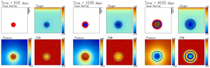
Fig. 2.

The evolution towards a steady-state avascular multicell (2D) spheroid. The tumour regions (black proliferating ΩP, dark grey hypoxic/quiescent ΩH, light grey necrotic ΩN), the oxygen, mechanical pressure and ECM are shown at times t = 0, 15 and 45 days. An animation is available with the supplementary materials
4.1 Avascular growth to a multicellular (2D) spheroid
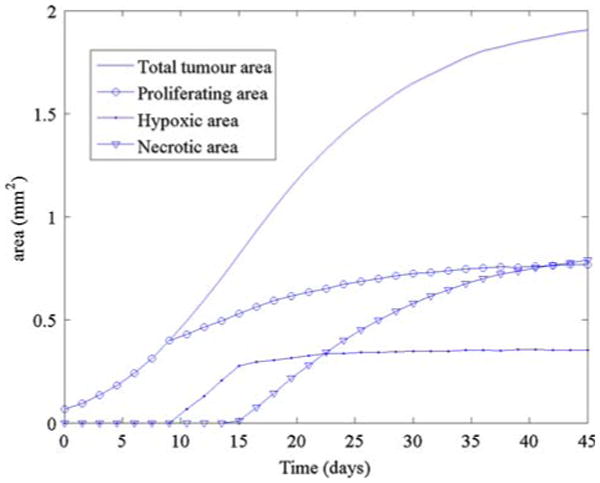
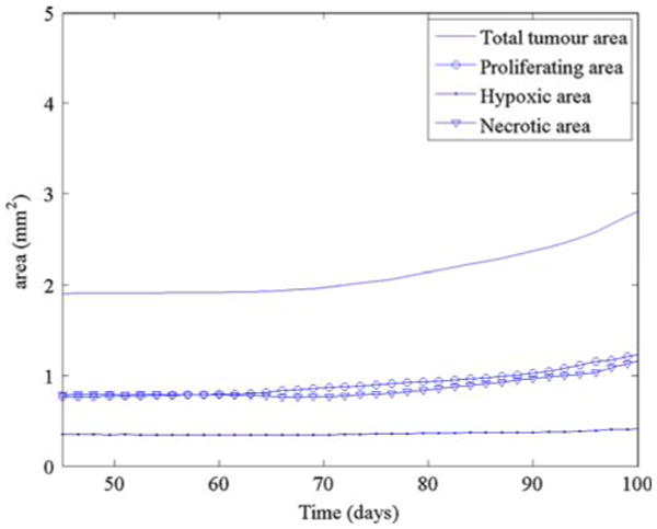
In Fig. 2, we present the growth of an avascular tumour. The spatial grid is 200 × 200 and the time step Δt = 0.05 which is adapted to satisfy the Courant–Friedrichs–Lewy (CFL) condition (see [45,46,48]). The red, blue and brown colors denote ΩP, ΩH, ΩN which are the proliferating, hypoxic/quiescent and necrotic regions, respectively. The non-dimensional oxygen and ECM concentrations and the solid (oncotic) pressure are also shown. The oxygen diffuses only a short distance (about 0.2 mm) from the parent vessel as can be observed from the figure. However, the pre-existing vasculature (which yields a background oxygen concentration of approximately 0.4), provides enough oxygen for the tumour to grow. As the tumour grows, the pressure in the proliferating region increases, the oxygen is depleted in the tumour and the ECM is degraded. A hypoxic/quiescent core forms at about 9 days when the tumour radius is approximately 0.34 mm (not shown). While the tumour continues to grow and degrade the extracellular matrix, the pressure decreases and the tumour growth starts to slow, as can be seen in Fig. 2. A necrotic core forms around day 15 when the radius of the tumour is approximately 0.5 mm. The pressure drops significantly to reflect the volume loss in the necrotic core associated with the break-down of the necrotic cells and the growth of the tumour slows even further as the tumour approaches a steady state. As the growth of the tumour slows, the ECM degradation becomes more pronounced. This actually causes a competition between two effects: the pressure-induced motion, which becomes more effective since the mobility increases when the ECM decreases, and haptotaxis which tends to inhibit growth of the tumour into the less dense ECM outside the tumour (recall that haptotaxis induces motion up ECM gradients). Further, the MDE also degrades the pre-existing vessels which results in a reduction in the supply of oxygen. As a result of haptotaxis and the reduced oxygen supply, the tumour actually shrinks slightly after reaching a maximum radius of about 0.64 mm, see Fig. 3.
Fig. 3.

The areas (mm2) of the total tumour (solid line), proliferating region (open circle), hypoxic region (closed dot) and the necrotic region (inverted triangle) as a function of time for the simulation in Fig. 2
4.2 Tumour-induced angiogenesis and vasular growth: no solid pressure-induced neovascular response
We next consider tumour-induced angiogenesis where there is no effect of the solid pressure on either the radius of the new vessels or the extravasation of nutrient. In particular, we take c (Pvessel, P) = 0 in Eqs. 4 and 25. Angiogenesis is initiated from the avascular tumour configuration at t = 45 days from Fig. 2. At this time, ten sprout tips are released from the parent vessel. The initial vessel radii are 6 μm. The inlet pressure and outlet pressures in the parent vessel are Pvessel,in = 3, 660 Pa and Pvessel,out = 2, 060 Pa, respectively. The growth duration is t = 0.05 which means that the intravascular flow and vessel adaption algorithms are called nearly every tumour growth time step. The flow duration is τ = 0.25 with a time step approximately equal to Δτ = 0.005 (again Δτ is adaptive to satisfy an intravascular CFL condition). This means that 50 iterations of the flow and vascular adaptation algorithms are performed every tumour growth time step. By flowing and adapting the vascular network so frequently, we hoped that a relatively short flow duration time could be used to get a reasonable approximation of the blood flow in the network. Indeed, preliminary simulations showed that increasing the flow duration did not change the results qualitatively or, in some cases depending on the vascular network configuration, quantitatively. In a future work, we will quantify the effect of the flow duration upon the results.
The evolution of the tumour and the neo-vascular network is shown in Figs. 4 and 5. As can be seen from the figures, it takes some time for flow to develop after angiogenesis is initiated; flow first occurs after about 7 days (52 days of total growth time) in a region near the parent vessel. This can be seen from the plots of haematocrit and oxygen which are signatures of blood flow. Little additional oxygen diffuses to the tumour. Accordingly, the tumour maintains a steady size (or shrinks a little due to the reasons described above). This may be seen in Fig. 6. Some of the vessels continue to lengthen, branch and migrate towards the tumour heading in particular for the hypoxic region where TAF is released.
Fig. 4.

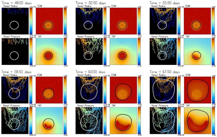
Tumour-induced angiogenesis and vascular tumour growth. The vessels do not respond to the solid pressure generated by the growing tumour. The tumour develops a microvascular network that provides it with a direct source of oxygen and results in rapid growth with a compact (sphere-like) shape. The colour scheme is the same as in Fig. 2 and the times shown are t = 48 (3 days after angiogenesis is initiated), 52.5, 55.5, 58.5, 63 and 67.5 days. An animation can be found online with the supplementary materials
Fig. 5.
Dimensional intravascular radius (m) and pressure (Pa) along with the nondimensional ECM and TAF concentrations from the simulation shown in Fig. 4. The times are the same as in Fig. 4
Fig. 6.

The areas (mm2) of the total tumour (solid line), proliferating region (open circle), hypoxic region (closed dot) and the necrotic region (inverted triangle) as a function of time for the simulation in Fig. 4
After about 10 days (55 days of total growth time), a large loop forms through which blood flows. The loop penetrates the tumour and provides the tumour cells with a direct source of oxygen. The tumour responds by rapidly growing along the oxygen source and co-opts the neo-vasculature and the hypoxic region shrinks and changes shape. As the tumour grows, the hypoxic and necrotic regions start to grow again as well and the new vessels near the tumour/host interface branch in response to wall shear stresses and increased TAF levels. This results in increased anastomosis and blood flow. The increased oxygen supply in turn causes large pressures to form in the proliferating region and the tumour to grow even more rapidly, enhancing this effect. Because there is no response of the new vessels to these large pressures, the tumour simply continues to co-opt the vessels creating an effective tumour microvasculature. This microvasculature provides a nearly uniform source of nutrient in the upper two thirds of the tumour; the lower third is primarily hypoxic and quiescent. As a consequence, the tumour shape remains compact as the tumour grows.
In Fig. 5, the dimensional neo-vasculature radii (in m) and intravascular pressures (in Pa) are shown together with the non-dimensional ECM and TAF concentrations. At early times, the radii are small and TAF diffuses from the quiescent zone. The ring of lowered ECM surrounding the tumour is clearly seen. The pressure is highest in the neo-vasculature closest to the inlet of the parent capillary where the highest pressures are. As blood flow starts, the radii increase and the overall pressure decreases while the pressure in some vessels increases as blood spreads throughout the network. This process continues as the tumour grows and the vasculature continues to branch, anastomose and carry more and more flow. As the hypoxic and necrotic regions shrink, the TAF distribution changes and the vessels respond accordingly. Observe that the degraded ECM just outside the tumour does not prevent the vessels from penetrating the tumour even though the sprout-tips have to migrate up ECM gradients to accomplish this.
The first vessels that penetrate the tumour do not carry blood and thus the tumour does not respond to their penetration. Instead, these vessels migrate towards the hypoxic region where they tend to get stuck. This occurs because the TAF concentration is nearly uniform (T = 1) and so the sprout-tips to move randomly and tend to collide with their own trailing vessel preventing further migration. At later times though, new vessels grow into the tumour center and anastomose. This leads to blood flow and oxygen extravasation deep in the tumour interior. Further, observe that the tumour grows so fast that it outruns the ring of degraded ECM around its boundary and is growing into only very slightly degraded ECM. The ECM in the tumour interior degrades rather slowly and the ECM signature of the original avascular tumour spheroid can still be seen at late times.
This simulation shows that when the new vessels are not affected by the tumour solid pressure, dramatic growth occurs as the tumour co-opts the host vasculature to create its own microvasculature and receives a direct source of oxygen. In addition, the tumour growth and angiogenesis processes are nonlinearly coupled as the vasculature responds to the growth by migrating towards the ever changing TAF distributions and by branching and anastomosing near the tumour–host interface. This leads to increased blood flow. At the same time, the increased blood flow in the vascular network affects how the tumour grows, and in particular speeds growth up. This then affects the response of the vasculature.
4.3 Tumour-induced angiogenesis and vasular growth: the effect of solid pressure-induced neovascular response
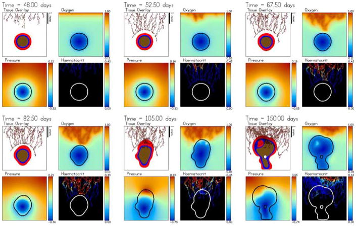
Next, we consider, in Figs. 7, 8 and 9, the effect of solid/mechanical pressure-induced vascular response on tumour-induced angiogenesis and vascular growth. We repeat the simulation in Sect. 4.2 except with c (Pvessel, P) non-zero as given in Eq. 5. This means that transfer of oxygen from the neo-vasculature to the tissue may be significantly reduced and the vessel radii may be correspondingly constricted. With the values of the parameters used here (see the supplementary materials), a solid pressure-induced vascular response begins to occur when the solid pressure P ≈ 0.8.
Fig. 7.

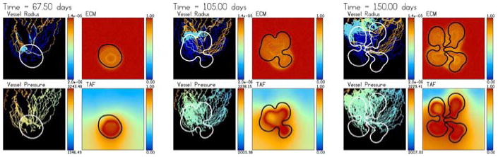
Tumour-induced angiogenesis and vascular tumour growth. The vessels respond to the solid pressure generated by the growing tumour. Accordingly, strong oxygen gradients are present that result in strongly heterogeneous tumour cell proliferation and shape instability. The color scheme is the same as in Fig. 2 and the times shown are t = 48 (3 days after angiogenesis is initiated), 52.5, 67.5, 82.5, 105 and 150 days. An animation is available online with the supplementary materials
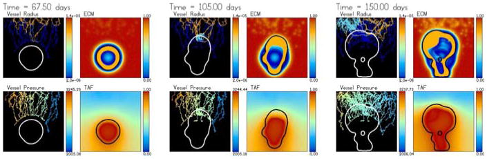
Fig. 8.
Dimensional intravascular radius (m) and pressure (Pa) along with the nondimensional ECM and TAF concentrations from the simulation shown in Fig. 7. The times are the same as in Fig. 7
Fig. 9.

The areas (mm2) of the total tumour (solid line), proliferating region (open circle), hypoxic region (closed dots) and the necrotic region (inverted triangle) as a function of time for the simulation in Fig. 7
At early times, the angiogenic response and the tumour growth is similar to the case presented earlier in Figs. 4, 5 and 6. The newly developing vessels migrate, proliferate, branch and anastomose. It also takes some time for flow to begin with significant flow developing only after about 10 days (55 days of total growth time). Blood flow in the neo-vasculature starts near the parent capillary and eventually the flow reaches the tumour. Because the initial ECM is slightly different than that in Fig. 4 (due to the random component) and due to the random component of the sprout tip motion, the vascular network at early times is not identical to that obtained previously in Fig. 4.
In contrast to the case considered in Fig. 4, here the solid pressure prevents any delivery of oxygen internally to the tumour and thus the delivery of oxygen is heterogeneous and significant oxygen gradients persist in the tumour interior. There is no functional microvasculature internal to the tumour. While the tumour responds by growing towards the oxygen-delivering neo-vasculature, the solid pressure generated by tumour cell proliferation also constricts the neo-vasculature in the direction of growth (where pressure is highest) and also correspondingly inhibits the transfer of oxygen from those vessels. As a consequence, the overall solid pressure is significantly lower than that in Fig. 4. This makes the tumour grow much more slowly than that in Fig. 4 as can be seen in Fig. 9. Note the vertical scale in Fig. 9 is one half of that in Fig. 6.
The neo-vasculature in other areas of the host microenvironment then provide a stronger source of oxygen. This triggers tumour-cell proliferation and growth in regions where proliferation had been decreased previously. The heterogeneity of oxygen delivery and the associated oxygen gradients cause heterogeneous tumour cell proliferation. Unlike the case in Fig. 4, proliferation is confined to regions close to the tumour–host interface. This results in morphological instability that leads to the formation of invasive tumour clusters (e.g. buds) and a complex tumour morphology. This result is consistent with the theory and predictions made earlier (see, for example, Cristini et al. [20,22,42], Anderson et. al. [3,5,30], and Macklin and Lowengrub [45–48]), that substrate inhomogeneities in the tumour microenvironment tend to cause morphological instabilities in growing tumours.
Although nutrient-providing, functional vessels are not able to penetrate the tumour during growth, the growth of the tumour elicits a strong branching and anastomosis response from the nearby neo-vasculature in the host microenvironment. Although there is an analogous neo-vascular response seen in Fig. 4, the effect here is much more pronounced as the levels of TAF are higher in these regions (because tumour hypoxia is increased) and thus the wall shear stresses initiate more significant branching.
In Fig. 8, the dimensional neo-vasculature radii (in m) and intravascular pressures (in Pa) are shown together with the non-dimensional ECM and TAF concentrations. As before, blood flow causes a dilation of the vessels and an overall decrease of pressure as branching, anastomosis and increased blood flow occurs throughout the neo-vascular network. The constriction of neo-vessels in response to the solid pressure is clearly seen.
The tumour-secreted MDE degrades the ECM in the host microenvironment near the tumour and in the tumour interior. As before (recall Fig. 5), the new vessels are still able to migrate through the region of lower ECM even though this acts against haptotaxis. Because the tumour grows more slowly than that in Fig. 5, only the tips of the invasive clusters outrun the degraded ECM. As can be seen in Fig. 8, the host ECM is degraded in the region between the invading clusters. The ECM signature of the original avascular tumour spheroid can no longer be seen at later times.
This simulation shows even stronger nonlinear coupling between the tumour-induced angiogenesis and the progression of the tumour compared to the prior case shown in Fig. 7, 8 and 9. The pressure-induced vascular response of constricting the radii of the neo-vasculature and inhibiting blood-tissue oxygen transfer not only affects the tumour growth dramatically, but also significantly affects the growth of the neo-vascular network, and vice-versa.
4.4 Avascular growth to a multicellular (2D) spheroid with enhanced ECM degradation and production
We next examine the effect of ECM degradation upon the results. In Fig. 10, we repeat the simulation in Sect. 4.1 except that both the MDE degradation and production parameters are increased (see the supplementary materials).
Fig. 10.
The evolution towards a steady-state avascular multicell (2D) spheroid with enhanced ECM degradation. The MDE production and degradation parameters are larger than those used in Fig. 2. See the supplementary materials where there is also an animation available online. The times shown are t = 0, 15 and 45 days
The tumour grows by uptaking oxygen delivered by the pre-existing (uniform) vasculature and growth is more rapid than that for the avascular tumour shown in Sect. 4.1 (Fig. 2). This occurs because the mobility is larger here due to the enhanced degradation of ECM. This effect overcomes the tendency of haptotaxis to keep the tumour away from the degraded ECM.
The tumour reaches a nearly steady size, containing both a hypoxic and a necrotic core, that is significantly larger than that shown in Figs. 2 and 3; the radius at 45 days is approximately 0.78 mm (see Fig. 11). At the final time shown (45 days), the ECM is significantly degraded in the host microenvironment and in the tumour necrotic core to the point that there is even a thin annular “hole” in the ECM immediately surrounding the spheroid, and a circular hole in the necrotic region where the density of ECM E ≈ 0.
Fig. 11.
The areas (mm2) of the total tumour (solid line), proliferating region (open circle), hypoxic region (solid dot) and the necrotic region (inverted triangle) as a function of time for the simulation in Fig. 10
4.5 Tumour-induced angiogenesis and vascular growth: The effect of solid pressure-induced neovascular response and enhanced ECM degradation and production
Next, we consider, in Figs. 12, 13 and 14, the effect of enhanced ECM degradation on tumour-induced angiogenesis and vascular growth. We repeat the simulation shown in Sect. 4.3 except that the initial condition is the t = 45 day simulation from Fig. 10 and the MDE parameters are the same as in that figure. (See the supplementary materials for the parameter values.)
Fig. 12.
Tumour-induced angiogenesis and vascular tumour growth with enhanced ECM degradation. The times shown are t = 48 (3 days after angiogenesis is initiated), 52.5, 67.5, 82.5, 105 and 150 days. An animation is available online with the supplementary materials
Fig. 13.
Dimensional intravascular radius (m) and pressure (Pa) along with the nondimensional ECM and TAF concentrations from the simulation in Fig. 12. The times are the same as in Fig. 12
Fig. 14.
The areas (mm2) of the total tumour (solid line), proliferating region (open circle), hypoxic region (solid dot) and the necrotic region (inverted triangle) as a function of time for the simulation in Fig. 12
As in the simulation shown in Sect. 4.2, the new vessels grow and form loops near the parent capillary. However, now because of the growing ECM annular hole surrounding the tumour, the new vessels are not able to reach the tumour and are instead trapped by the ECM hole due to haptotaxis. The vessels then encapsulate roughly the upper half of the tumour.
As blood flows through the neo-vascular network and approaches the tumour, the tumour responds by growing towards the flowing neo-vasculature that provide the oxygen source, as in Sect. 4.3. The tumour elongates, constricts the neo-vasculature in its path and prevents the transfer of oxygen from the neo-vasculature to the host. This limits tumour cell proliferation and results in a roughly steady maximum solid pressure. Correspondingly, there is heterogeneous oxygen supply, heterogeneous tumour cell proliferation and there are strong oxygen gradients. As in Sect. 4.3, this results in a morphological instability of the growing solid tumour.
As the tumour continues to grow, the neo-vasculature respond by increasing branching and anastomosing near the tumour–host interface; similar dense blood vessel growth near the tumour periphery has been observed clinically in glioma [35]. The denser vascular network results in a broader supply of oxygen in the part of the tumour closest to the parent capillary. Proliferation is increased and the top of the tumour flattens. The increased proliferation leads to large solid pressures which then constrict the nearby new vessels and inhibit oxygen supply. The tumour then begins to grow towards other vessels near the parent capillary and the top of the tumour becomes unstable. Further, there is instability along the side of the tumour that leads to the encapsulation of host domain inside the tumour. Also observe that a small amount of oxygen is able to be delivered into the tumour interior at very late times as haematocrit is trapped in a constricted vessel at a location where the pressure is sufficiently low to allow extravasation.
Figure 13 shows the dimensional neo-vasculature radii (in m) and the intravascular pressures (in Pa) together with the non-dimensional ECN and TAF concentrations. The results are similar to those obtained before except that the tumour does not outrun the ECM hole although at the top of the tumour, the hole is quite shallow.
Interestingly, even though the initial tumour in Fig. 12 is larger than that in Fig. 7, the final tumour size at t = 150 days is roughly the same for both cases (see Figs. 14 and 9). The ECM hole present in the simulation in Fig. 12 prevents the new vessels from getting close to the tumour during the early stages of growth; this allows the tumour in Fig. 7 to catch up and even grow slightly larger than that in Fig. 12.
Furthermore, the enhanced matrix degradation increases the mobility μ in the tumour microenvironment relative to inside the tumour, resulting in a biomechanically responsive microenvironment; the observed relatively compact morphology is consistent with the predictions of Macklin and Lowengrub in [47] for this growth regime. (See the analogous tumor-shapes in the upper row of the morphology diagram in Fig. 15, compared with the upper right plot). Similarly, the lower matrix degradation in Sect. 4.3 decreases the mobility in the tumour microenvironment relative to the tumour, yielding a biomechanically-unresponsive microenvironment; the observed fingering morphology matches the predictions in [47] for this growth regime. (Compare the tumor-shapes in the lower right figures of the morphology diagram in Fig. 15 with the lower right plot).
Fig. 15.
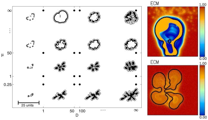
Left predicted tumour morphological response to microenvironmental nutrient availability (increases along horizontal axis) and biomechanical responsiveness (increases along vertical axis) from [47] (reprinted with permission from Elsevier). Right Tumour morphology and ECM profile at 150 days with enhanced matrix degradation (top, Sect. 4.5) and lower matrix degradation (bottom, Sect. 4.3)
Finally, in Fig. 16, we compare the average radii in the neo-vascular networks for the simulations in Figs. 4, 7 and 12. At early times, the radii for the simulation in Fig. 4, where the neo-vasculature does not respond to solid pressure, grows the fastest as blood flows uninhibited through the network. Later, however, the simulation with lower ECM degradation shows the most rapid radii increase. This occurs because the EC sprout-tips are able to move more freely through the host domain and do not get caught by degraded ECM. This provides the vascular network with a more widely varying flow response.
Fig. 16.
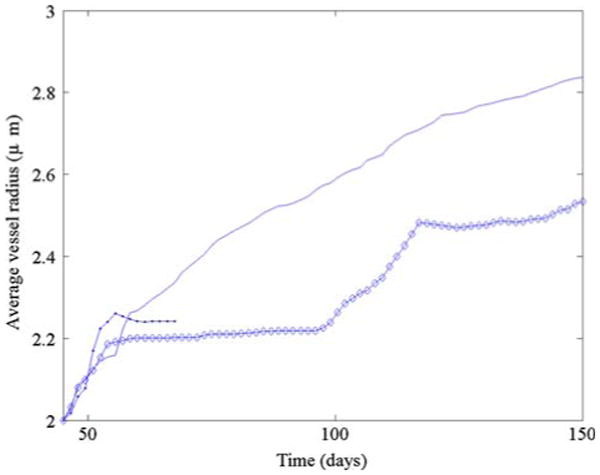
Average vessel radii. Simulation from Fig. 7 (solid), simulation from Fig. 4. (solid dots), simulation from Fig. 12 (diamond)
5 Conclusions and future directions
In this paper, we have coupled an improved continuum model of solid tumour invasion (following [48]) with a model of tumour-induced angiogenesis (following [50]) to produce a new multi-scale model of vascular solid tumour growth. The invasion and angiogenesis models were coupled through the tumour angiogenic factors (TAF) released by the tumour cells and through the nutrient extravasated from the neo-vascular network. As the blood flows through the neo-vascular network, nutrients (e.g. oxygen) are extravasated and diffuse through the ECM triggering further growth of the tumour, which in turn influences the TAF expression. In addition, the extravasation is mediated by the hydrostatic stress (solid pressure) generated by the growing tumour. The solid pressure also affects vascular remodeling by restricting the radii of the vessels and thus the flow pattern and wall shear stresses. The vascular network and tumour progression were also coupled via the ECM as both the tumour cells and ECs upregulate matrix degrading proteolytic enzymes which cause localized degradation of the ECM which in turn affects haptotactic migration.
We performed simulations of the multi-scale model that demonstrated the importance of the nonlinear coupling between the growth and remodeling of the vascular network, the blood flow through the network and the tumour progression. The solid pressure generated by tumour cell proliferation effectively shuts down large portions of the vascular network dramatically affecting the flow, the subsequent network remodeling, the delivery of nutrients to the tumour and the subsequent tumour progression. In addition, ECM degradation by tumour cells was seen to have a dramatic affect on both the development of the vascular network and the growth response of the tumour. In particular, when the ECM degradation is significant, the newly formed vessels tended to encapsulate, rather than penetrate, the tumour and were thus less effective in delivering nutrients.
There are many directions in which this work will be taken in the future both in terms of modeling additional biophysical effects as well as algorithmic improvements. Regarding the algorithm, we plan to upgrade the solid pressure/nutrient solver by solving for P and σ as a coupled system. This will prevent oscillations that may occur by lagging P in the source term for nutrient. We also plan to accelerate the solver for the intravascular pressure to improve performance of the coupled algorithm.
Regarding the model, we plan to develop a more detailed analysis of the effect of solid pressure on the constriction and collapse of vessels in the microvasculature and on the corresponding response of the microvascular network. We also plan to include the effects of the venous system. Other features, such as the recruitment of pericytes by the vascular ECs will also be investigated. In addition, we will incorporate more realistic models for soft tissue mechanics.
The work presented here demonstrates that nonlinear simulations are a powerful tool for understanding phenomena fundamental to solid tumour growth. A biophysically justified computer model could provide an enormous benefit to the clinician, the patient, and society by efficiently searching parameter space to identify optimal, or nearly optimal, individualized treatment strategies involving, for example, chemotherapy and adjuvant treatments such as anti-angiogenic or anti-invasive therapies. This is a direction we plan to explore in the future.
Supplementary Material
Acknowledgments
PM, VC and JL are grateful to Hermann Frieboes for valuable discussions. We thank the reviewers for their comments and helpful suggestions on shortening the manuscript. PM acknowledges partial support from a US Department of Education GAANN (Graduate Assistance in Areas of National Need) fellowship. MC was supported by a Leverhulme Trust Personal Research Fellowship. VC acknowledges partial support from the National Science Foundation (NSF) and the National Institutes of Health (NIH) through grants NSF-DMS-0314463 and NIH-5R01CA093650-03. JL acknowledges partial support from the NSF through grants DMS-0352143 and DMS-0612878 and from the NIH through grant P50GM76516 for a Center of Excellence in Systems Biology at UCI.
Footnotes
Mathematics Subject Classification (2000) 62P10
Contributor Information
Paul Macklin, School of Health Information Sciences, University of Texas Health Science Center, Houston, USA, paul.t.macklin@uth.tmc.edu, URL: http://biomathematics.shis.uth.tmc.edu.
Steven McDougall, Institute of Petroleum Engineering, Heriot-Watt University, Edinburgh, Scotland, UK, steve.mcdougall@pet.hw.ac.uk, URL: http://www.pet.hw.ac.uk/aboutus/staff/pages/mcdougall_s.htm.
Alexander R. A. Anderson, Division of Mathematics, University of Dundee, Dundee, Scotland, UK, anderson@maths.dundee.ac.uk, URL: http://www.maths.dundee.ac.uk/∼sanderso/
Mark A. J. Chaplain, Division of Mathematics, University of Dundee, Dundee, Scotland, UK, chaplain@maths.dundee.ac.uk, URL: http://www.maths.dundee.ac.uk/∼chaplain/
Vittorio Cristini, School of Health Information Sciences, University of Texas Health Science Center, Houston, USA; M.D. Anderson Cancer Center, Houston, TX, USA, Vittorio.cristini@uth.tmc.edu, URL: http://cristinilab.shis.uth.tmc.edu.
John Lowengrub, Mathematics Department, University of California, Irvine, CA 92697-3875, USA, lowengrb@math.uci.edu, URL: http://math.uci.edu/∼lowengrb.
References
- 1.Alarcón T, Byrne HM, Maini PK. A multiple scale model for tumor growth. Multiscale Model Simul. 2005;3:440–475. [Google Scholar]
- 2.Ambrosi D, Preziosi L. On the closure of mass balance models for tumor growth. Math Model Meth Appl Sci. 2002;12(5):737–754. [Google Scholar]
- 3.Anderson ARA. A hybrid mathematical model of solid tumour invasion: the importance of cell adhesion. IMA Math App Med Biol. 2005;22(2):163–186. doi: 10.1093/imammb/dqi005. [DOI] [PubMed] [Google Scholar]
- 4.Anderson ARA, Chaplain MAJ. Continuous and discrete mathematical models of tumor-induced angiogenesis. Bull Math Biol. 1998;60(5):857–900. doi: 10.1006/bulm.1998.0042. [DOI] [PubMed] [Google Scholar]
- 5.Anderson ARA, Weaver AM, Cummings PT, Quaranta V. Tumor morphology and phenotypic evolution driven by selective pressure from the microenvironment. Cell. 2006;127(5):905–915. doi: 10.1016/j.cell.2006.09.042. [DOI] [PubMed] [Google Scholar]
- 6.Araujo RP, McElwain DLS. A history of the study of solid tumor growth: the contribution of mathematical modeling. Bull Math Biol. 2004;66(5):1039–1091. doi: 10.1016/j.bulm.2003.11.002. [DOI] [PubMed] [Google Scholar]
- 7.Araujo RP, McElwain DLS. A mixture theory for the genesis of residual stresses in growing tissues I: a general formulation. SIAM J Appl Math. 2005;65:1261–1284. [Google Scholar]
- 8.Araujo RP, McElwain DLS. A mixture theory for the genesis of residual stresses in growing tissues II: solutions to the biphasic equations for a multicell spheroid. SIAM J Appl Math. 2005;66(2):447–467. [Google Scholar]
- 9.Balding D, McElwain DLS. A mathematical model of tumour-induced capillary growth. J Theor Biol. 1985;114:53–73. doi: 10.1016/s0022-5193(85)80255-1. [DOI] [PubMed] [Google Scholar]
- 10.Bartha K, Rieger H. Vascular network remodeling via vessel cooption, regression and growth in tumors. J Theor Biol. 2007;241(4):903–918. doi: 10.1016/j.jtbi.2006.01.022. [DOI] [PubMed] [Google Scholar]
- 11.Byrne H, Preziosi L. Modelling solid tumour growth using the theory of mixtures. Math Med Biol. 2003;20(4):341–366. doi: 10.1093/imammb/20.4.341. [DOI] [PubMed] [Google Scholar]
- 12.Byrne HM, Alarcón T, Owen MR, Webb SD, Maini PK. Modeling aspects of cancer dynamics: a review. Phil Trans R Soc A. 2006;364(1843):1563–1578. doi: 10.1098/rsta.2006.1786. [DOI] [PubMed] [Google Scholar]
- 13.Byrne HM, Chaplain MAJ. Growth of non-necrotic tumours in the presence and absence of inhibitors. Math Biosci. 1995;130:151–181. doi: 10.1016/0025-5564(94)00117-3. [DOI] [PubMed] [Google Scholar]
- 14.Byrne HM, Chaplain MAJ. Growth of necrotic tumours in the presence and absence of inhibitors. Math Biosci. 1996;135:187–216. doi: 10.1016/0025-5564(96)00023-5. [DOI] [PubMed] [Google Scholar]
- 15.Byrne HM, Chaplain MAJ. Free boundary problems arising in models of tumour growth and development. Eur J Appl Math. 1998;8:639–658. [Google Scholar]
- 16.Carmeliet P. Angiogenesis in life, disease, and medicine. Nature. 2005;438:932–936. doi: 10.1038/nature04478. [DOI] [PubMed] [Google Scholar]
- 17.Chaplain MAJ. The mathematical modelling of tumour angiogenesis and invasion. Acta Biotheor. 1995;43:387–402. doi: 10.1007/BF00713561. [DOI] [PubMed] [Google Scholar]
- 18.Chaplain MAJ, McDougall SR, Anderson ARA. Mathematical modelling of tumor-induced angiogenesis. Annu Rev Biomed Eng. 2006;8:233–257. doi: 10.1146/annurev.bioeng.8.061505.095807. [DOI] [PubMed] [Google Scholar]
- 19.Chomyak OG, Sidorenko MV. Multicellular spheroids model in oncology. Exp Oncol. 2001;23:236–241. [Google Scholar]
- 20.Cristini V, Frieboes HB, Gatenby R, Caserta S, Ferrari M, Sinek J. Morphological instability and cancer invasion. Clin Cancer Res. 2005;11(19):6772–6779. doi: 10.1158/1078-0432.CCR-05-0852. [DOI] [PubMed] [Google Scholar]
- 21.Cristini V, Li X, Lowengrub J, Wise S. Nonlinear simulations of solid tumor growth using a mixture model: invasion and branching. J Math Biol. 2008 doi: 10.1007/s00285-008-0215-x. in press. [DOI] [PMC free article] [PubMed] [Google Scholar]
- 22.Cristini V, Lowengrub JS, Nie Q. Nonlinear simulation of tumor growth. J Math Biol. 2003;46:191–224. doi: 10.1007/s00285-002-0174-6. [DOI] [PubMed] [Google Scholar]
- 23.Dickinson RB, Tranquillo RT. A stochastic model for adhesion-mediated cell random motility and haptotaxis. J Math Biol. 1993;31:563–600. doi: 10.1007/BF00161199. [DOI] [PubMed] [Google Scholar]
- 24.DiMilla PA, Barbee K, Lauffenburger DA. Mathematical model for the effects of adhesion and mechanics on cell migration speed. Biophys J. 1991;60:15–37. doi: 10.1016/S0006-3495(91)82027-6. [DOI] [PMC free article] [PubMed] [Google Scholar]
- 25.Erler JT, Bennewith KL, Nicolau M, Dornhöfer N, Kong C, Le QT, Chi JTA, Jeffrey SS, Giaccia AJ. Lysyl oxidase is essential for hypoxia-induced metastasis. Nature. 2006;440(27):1222–1226. doi: 10.1038/nature04695. [DOI] [PubMed] [Google Scholar]
- 26.Frieboes HB, Lowengrub JS, Wise S, Zheng X, Macklin P, Cristini V. Computer simulations of glioma growth and morphology. NeuroImage. 2007;37(S1):S59–S70. doi: 10.1016/j.neuroimage.2007.03.008. [DOI] [PMC free article] [PubMed] [Google Scholar]
- 27.Frieboes HB, Zheng X, Sun CH, Tromberg B, Gatenby R, Cristini V. An integrated computational/experimental model of tumor invasion. Can Res. 2006;66(3):1597–1604. doi: 10.1158/0008-5472.CAN-05-3166. [DOI] [PubMed] [Google Scholar]
- 28.Friedl P, Wolf K. Tumour-cell invasion and migration: diversity and escape mechanisms. Nat Rev Cancer. 2003;3:362–374. doi: 10.1038/nrc1075. [DOI] [PubMed] [Google Scholar]
- 29.Galaris D, Barbouti A, Korantzopoulos P. Oxidative stress in hepatic ischemia–reperfusion injury: the role of antioxidants and iron chelating compounds. Curr Pharm Des. 2006;12(23):2875–2890. doi: 10.2174/138161206777947614. [DOI] [PubMed] [Google Scholar]
- 30.Gerlee P, Anderson ARA. Stability analysis of a hybrid cellular automaton model of cell colony growth. Phys Rev E. 2007;75:0151,911. doi: 10.1103/PhysRevE.75.051911. [DOI] [PubMed] [Google Scholar]
- 31.Graziano L, Preziosi L. Mechanics in tumor growth. In: Mollica F, Rajagopal KR, Preziosi L, editors. Modelling of Biological Materials. Birkhäuser; Boston: 2007. pp. 267–328. [Google Scholar]
- 32.Greenspan HP. On the growth and stability of cell cultures and solid tumors. J Theor Biol. 1976;56(1):229–242. doi: 10.1016/s0022-5193(76)80054-9. [DOI] [PubMed] [Google Scholar]
- 33.Hanahan D, Weinberg RA. The hallmarks of cancer. Cell. 2000;100(1):57–70. doi: 10.1016/s0092-8674(00)81683-9. [DOI] [PubMed] [Google Scholar]
- 34.Hogea CS, Murray BT, Sethian JA. Simulating complex tumor dynamics from avascular to vascular growth using a general level-set method. J Math Biol. 2006;53(1):86–134. doi: 10.1007/s00285-006-0378-2. [DOI] [PubMed] [Google Scholar]
- 35.Holash J, Weigand SJ, Yancopoulos GD. New model of tumor-induced angiogenesis; dynamic balance between vessel regresion and growth mediated by angiopoietins and vegf. Oncogene. 1999;18:5356–5362. doi: 10.1038/sj.onc.1203035. [DOI] [PubMed] [Google Scholar]
- 36.Kaur B, Khwaja FW, Severson EA, Matheny SL, Brat DJ, Van Meir EG. Hypoxia and the hypoxia-inducible-factor pathway in glioma growth and angiogenesis. Neuro-oncology. 2005;7(2):134–153. doi: 10.1215/S1152851704001115. [DOI] [PMC free article] [PubMed] [Google Scholar]
- 37.Kim JB. Three-dimensional tissue culture models in canceriology. J Biomol Screen. 2005;15:365–377. doi: 10.1016/j.semcancer.2005.05.002. [DOI] [PubMed] [Google Scholar]
- 38.Kloner RA, Jennings RB. Consequences of brief ischemia: stunning, preconditioning, and their clinical implications: part 1. Circulation. 2001;104(24):2981–2989. doi: 10.1161/hc4801.100038. [DOI] [PubMed] [Google Scholar]
- 39.Kunz-Schughart LA, Freyer JP, Hofstaedter F, Ebner R. The use of 3-d cultures for high-throughput screening: the multicellular spheroid model. J Biomol Screen. 2004;9:273–285. doi: 10.1177/1087057104265040. [DOI] [PubMed] [Google Scholar]
- 40.Lauffenburger DA, Horwitz AF. Cell migration: a physically integrated molecular process. Cell. 1996;84(3):359–369. doi: 10.1016/s0092-8674(00)81280-5. [DOI] [PubMed] [Google Scholar]
- 41.Lee D, Rieger H. Flow correlated percolation during vascular remodeling in growing tumors. Phys Rev Lett. 2006;96:058,104. doi: 10.1103/PhysRevLett.96.058104. [DOI] [PubMed] [Google Scholar]
- 42.Li X, Cristini V, Nie Q, Lowengrub J. Nonlinear three-dimensional simulation of solid tumor growth. Disc Dyn Contin Dyn Syst B. 2007;7:581–604. [Google Scholar]
- 43.Liotta LA, Clair T. Checkpoint for invasion. Ann Ital Med Int. 2000;15(3):195–198. [Google Scholar]
- 44.Liotta LA, Stetler-Stevenson WG. Tumor cell motility. Sem Canc Biol. 1991;2(2):111–114. [PubMed] [Google Scholar]
- 45.Macklin P, Lowengrub JS. Evolving interfaces via gradients of geometry-dependent interior Poisson problems: application to tumor growth. J Comput Phys. 2005;203(1):191–220. [Google Scholar]
- 46.Macklin P, Lowengrub JS. An improved geometry-aware curvature discretization for level set methods: application to tumor growth. J Comput Phys. 2006;215(2):392–401. [Google Scholar]
- 47.Macklin P, Lowengrub JS. Nonlinear simulation of the effect of microenvironment on tumor growth. J Theor Biol. 2007;245(4):677–704. doi: 10.1016/j.jtbi.2006.12.004. [DOI] [PubMed] [Google Scholar]
- 48.Macklin P, Lowengrub JS. A new ghost cell/level set method for moving boundary problems: Application to tumor growth. J Sci Comput. 2008 doi: 10.1007/s10915-008-9190-z. in press. [DOI] [PMC free article] [PubMed] [Google Scholar]
- 49.Mantzaris NV, Webb S, Othmer HG. Mathematical modeling of tumor-induced angiogenesis. J Math Biol. 2004;49:111–187. doi: 10.1007/s00285-003-0262-2. [DOI] [PubMed] [Google Scholar]
- 50.McDougall SR, Anderson ARA, Chaplain MAJ. Mathematical modelling of dynamic adaptive tumour-induced angiogenesis: clinical implications and therapeutic targeting strategies. J Theor Biol. 2006;241(3):564–589. doi: 10.1016/j.jtbi.2005.12.022. [DOI] [PubMed] [Google Scholar]
- 51.McDougall SR, Anderson ARA, Chaplain MAJ, Sherratt JA. Mathematical modelling of flow through vascular networks: implications for tumour-induced angiogenesis and chemotherapy strategies. Bull Math Biol. 2002;64(4):673–702. doi: 10.1006/bulm.2002.0293. [DOI] [PubMed] [Google Scholar]
- 52.Orme ME, Chaplain MAJ. A mathematical model of vascular tumour growth and invasion. Math Comp Modell. 1996;23:43–60. [Google Scholar]
- 53.Palecek SP, Loftus JC, Ginsberg MH, Lauffenburger DA, Horwitz AF. Integrin-ligand binding properties govern cell migration speed through cell-substratum adhesiveness. Nature. 1997;385:537–540. doi: 10.1038/385537a0. [DOI] [PubMed] [Google Scholar]
- 54.Paweletz N, Knierim M. Tumor-related angiogenesis. Crit Rev Oncol Hematol. 1989;9:197–242. doi: 10.1016/s1040-8428(89)80002-2. [DOI] [PubMed] [Google Scholar]
- 55.Plank MJ, Sleeman BD. Lattice and non-lattice models of tumour angiogenesis. Bull Math Biol. 2004;66:1785–1819. doi: 10.1016/j.bulm.2004.04.001. [DOI] [PubMed] [Google Scholar]
- 56.Pouysségur J, Dayan F, Mazure NM. Hypoxia signalling in cancer and approaches to enforce tumour regression. Nature. 2006;441(25):437–443. doi: 10.1038/nature04871. [DOI] [PubMed] [Google Scholar]
- 57.Pries AR, Reglin B, Secomb TW. Structural adaptation of microvascular networks: functional roles of adaptive responses. Am J Physiol Heart Circ Physiol. 2001;281:H1015–H1025. doi: 10.1152/ajpheart.2001.281.3.H1015. [DOI] [PubMed] [Google Scholar]
- 58.Pries AR, Reglin B, Secomb TW. Structural adaptation of vascular networks: role of the pressure response. Hypertension. 2001;38:1476–1479. doi: 10.1161/hy1201.100592. [DOI] [PubMed] [Google Scholar]
- 59.Pries AR, Secomb TW, Gaehtgens P. Design principles of vascular beds. Circ Res. 1995;77:1017–1023. doi: 10.1161/01.res.77.5.1017. [DOI] [PubMed] [Google Scholar]
- 60.Pries AR, Secomb TW, Gaehtgens P. Biophysical aspects of blood flow in the microvasculature. Cardivasc Res. 1996;32:654–667. [PubMed] [Google Scholar]
- 61.Pries AR, Secomb TW, Gaehtgens P. Structural adaptation and stability of microvascular netwoks: theory and simulation. Am J Physiol Heart Circ Physiol. 1998;275(44):H349–H360. doi: 10.1152/ajpheart.1998.275.2.H349. [DOI] [PubMed] [Google Scholar]
- 62.Quaranta V, Weaver AM, Cummings PT, Anderson ARA. Mathematical modeling of cancer: the future of prognosis and treatment. Clin Chim Acta. 2005;357(2):173–179. doi: 10.1016/j.cccn.2005.03.023. [DOI] [PubMed] [Google Scholar]
- 63.Roose T, Chapman SJ, Maini PK. Mathematical models of avascular cancer. SIAM Rev. 2007;49:179–208. [Google Scholar]
- 64.Sanga S, Sinek JP, Frieboes HB, Fruehauf JP, Cristini V. Mathematical modeling of cancer progression and response to chemotherapy. Exp Rev Anticancer Ther. 2006;6(10):1361–1376. doi: 10.1586/14737140.6.10.1361. [DOI] [PubMed] [Google Scholar]
- 65.Sinek J, Frieboes H, Zheng X, Cristini V. Two-dimensional chemotherapy simulations demonstrate fundamental transport and tumor response limitations involving nanoparticles. Biomed Microdev. 2004;6(4):197–309. doi: 10.1023/B:BMMD.0000048562.29657.64. [DOI] [PubMed] [Google Scholar]
- 66.Stephanou A, McDougall SR, Anderson ARA, Chaplain MAJ. Mathematical modelling of flow in 2d and 3d vascular networks: applications to anti-angiogenic and chemotherapeutic drug strategies. Math Comput Modell. 2005;41:1137–1156. [Google Scholar]
- 67.Stéphanou A, McDougall SR, Anderson ARA, Chaplain MAJ. Mathematical modelling of the influence of blood rheological properties upon adaptive tumour-induced angiogenesis. Math Comp Model. 2006;44(1–2):96–123. [Google Scholar]
- 68.Thompson DW. On Growth and Form. Cambridge University Press; Cambridge: 1917. [Google Scholar]
- 69.Walles T, Weimer M, Linke K, Michaelis J, Mertsching H. The potential of bioartificial tissues in oncology research and treatment. Onkologie. 2007;30:388–394. doi: 10.1159/000102544. [DOI] [PubMed] [Google Scholar]
- 70.Welter M, Bartha K, Rieger H. Emergent vascular network inhomogenities and resulting blood flow patterns in a growing tumor. J Theor Biol. 2008;250:257–280. doi: 10.1016/j.jtbi.2007.09.031. [DOI] [PubMed] [Google Scholar]
- 71.Zheng X, Wise SM, Cristini V. Nonlinear simulation of tumor necrosis, neo-vascularization and tissue invasion via an adaptive finite-element/level set method. Bull Math Biol. 2005;67(2):211–259. doi: 10.1016/j.bulm.2004.08.001. [DOI] [PubMed] [Google Scholar]
Associated Data
This section collects any data citations, data availability statements, or supplementary materials included in this article.