On Combining Family–based and Population-based Case-control Data in Association Studies

Summary

Combining data collected from different sources can potentially enhance statistical efficiency in estimating effects of environmental or genetic factors or gene-environment interactions. However, combining data across studies becomes complicated when data are collected under different study designs, such as family-based and unrelated individual-based case-control design. In this paper, we describe likelihood based approaches that permit the joint estimation of covariate effects on disease risk under study designs that include cases, relatives of cases, and unrelated individuals. Our methods accommodate familial residual correlation and a variety of ascertainment schemes. Extensive simulation experiments demonstrate that the proposed methods for estimation and inference perform well in realistic settings. Efficiencies of different designs are contrasted in the simulation. We applied the methods to data from the Colorectal Cancer Family Registry.

1. Introduction

Associations between disease risk and genetic polymorphisms can be evaluated with two different study designs: population-based case-unrelated control studies and family-based studies. The population-based case-unrelated control study design has been the cornerstone of epidemiological association studies with less common and/or late onset diseases such as coronary heart disease and cancer. Population controls, genetically unrelated to the cases, are subject to genetic confounding such as population stratification. Family-based studies, on the other hand, using genotypes of blood relatives as references, are inherently robust to this type of bias. Because each type of design has its strengths and limitations, investigators sometimes conduct parallel studies using a variety of data resources (Newcomb et al., 2007; Landi et al., 2005).When both sources of information are available from the same underlying population, combining information from different sources may enhance statistical power in identifying important environmental risk factors and disease susceptibility genes.

The motivating example for our research comes from the Colorectal Cancer Family Registry (Colon CFR) (Newcomb et al., 2007). The Colon CFR is an international consortium formed to support studies of genetic and molecular epidemiology of colorectal cancer. Within the Colon CFR, colorectal cancer cases were identified in the six study sites using two strategies: a population-based recruitment where incident case probands were identified from cancer registries, or a clinic-based recruitment where families were recruited with multiple cases of colorectal cancer presenting at the cancer clinics. Controls were either randomly sampled from the general population within the relevant catchment area as cases, or from the family members of the cases. While such diverse data sources provide great research opportunities for identification and characterization of environmental risk factors and susceptibility genes, differences in sampling frame from the individual participating sites make appropriate analysis of this registry data as a whole challenging. The objective of this manuscript is to develop valid statistical estimation procedures for combining data collected from both population-based and family-based recruitment and for accommodating diverse ascertainment schemes that commonly found in association studies such as those conducted in Colon CFR.

The analysis of family data is complicated by two aspects of the data: potential familial residual correlation and the ascertainment scheme. Shared but unmeasured genetic or environmental factors may cause dependencies in disease risks among family members. Furthermore, as a strategy to improve efficiency when studying the association of a rare disease and a rare putative high-risk mutation, family designs often involve more complicated outcome-dependent ascertainment than a case-unrelated control study, for example, by only sampling family members of cases, or sampling heavily affected families ad hoc.

Methods that are appropriate for family-based studies have been developed in the last decade (Whittemore, 1995; Pfeiffer et al., 2001; Neuhaus et al., 2002). The most commonly used approach for family data is conditional logistic regression (CLR) for matched case-control studies (Breslow and Day, 1980). In the case of a family-based study, the likelihood conditions on the number of observed cases in each family, therefore it can accommodate any ascertainment scheme that is only related to phenotypes. However it is known that substantial information may be lost due to lack of proper controls as only disease and genotype discordant families are informative. For both CLR and random effects models, the regression coefficients are the log odds ratio (OR) relating the disease risk to covariates for individuals from the same family. Such estimates are not comparable to the OR estimated at the population level, and care must be taken when comparing the association estimated from a population-based case-unrelated control study with the family-specific effect that is estimated from a family-based study (Zeger et al., 1988).

In contrast, in the class of marginal models, regression coefficients represent the log odd ratios at population level regardless of the specific family from which an individual comes. Such models may be more attractive as a viable approach to be further compared or combined with data from population sampling. Different marginally specified models for family data have been proposed in the literature (Whittemore, 1995; Neuhaus et al., 2002). These marginal models treat an individual as an independent sampling unit and use robust variance estimates to accommodate within-family correlations. Both the retrospective covariate model of Whittemore and Halpern (2003) and the pseudoscore approach of Pfeiffer et al. (2008) relied on the assumption of independence conditional on measured covariates and family history, and can be potentially biased in the presence of further familial residual correlations.

Methods for combining data collected under different designs have received considerable attention recently (Slager and Schaid, 2001; Thornton and McPeek, 2007; Pfeiffer et al., 2008; Chen and Lin, 2008). Some of the existing work focuses on testing whether a genetic variant is associated with disease risk and does not always offer an approach for obtaining unbiased risk estimates. Methods that yield robust and efficient relative risk estimates at the population level are still lacking. In this paper we propose a likelihood based approach that yields efficient estimates. The key to our proposal is to first identify an appropriate model for family data that has the following characteristics: it accounts for familial residual correlations in a natural way; it flexibly incorporates a variety of ascertainment schemes commonly used in family studies; and perhaps most importantly, it provides estimates whose interpretation can be easily connected to those obtained from the analysis of case-unrelated control data collected at population level. Our proposed approach therefore can flexibly accommodate hybrid data that consist of population based cases, unrelated controls and either case of relatives. We provide detailed estimation procedures for both family data and combined data in Section 2. The performance of our proposed estimators is assessed numerically in Section 3. Efficiencies of different designs are contrasted under a few scenarios. The proposed method is illustrated with an analysis of data from the Colon CFR.

2. Methods

Consider a study where the data consist of a population based case-control sample of size n_P, with n₁ cases and n₀ unrelated controls, and a sample of n_F families. We allow n₁ cases to overlap with affected probands in the family component. Let D_k and X_k denote respectively the disease outcome and risk factors for the kth individual sampled retrospectively from the target population, and A_k = 1 if the kth subject is included in the sample. For family data, let D_ij, X_ij denote disease and vectors of covariates for the jth family member of the ith family with size m_i. For comparing and combining data from both resources, it is sensible to make inference at the level of subgroups defined by individual covariates. We therefore use a marginal logistic regression model to describe the relationship between covariates X_l and outcome D_l for an individual l from either data collection source:

$$\mathrm{logit}\{\mathrm{Pr}(D_l=1|{\mathbf{X}}_l)\}={\beta }_0+{\mathit{\beta }}_1{\mathbf{X}}_l,$$ (1)

where β₀ measures the baseline log-odds of disease risk for an individual with X = 0, and β₁ quantify the log-odds ratios (OR) of disease risk for a unit increment in components of X.

2.1 Likelihoods for Population-based Case-unrelated Control Studies

Population-based case-unrelated control studies entail retrospectively ascertaining covariate information on pre-selected cases and controls. The logistic model in equation (1) is specified for prospective sampling. It has been established that odds ratios can be consistently estimated from a case-unrelated control sample as if it had been prospectively collected in a hypothetical population (Anderson, 1972; Prentice and Pyke, 1979). The retrospective likelihood function ${ℒ}_p({\beta }_0^{\ast },\mathit{\beta })$ for the case-unrelated control sample can be written as

$$\mathbf{\prod }_{k=1}^{n_P}\mathrm{P}({\mathbf{X}}_k|D_k,A_k)\propto \mathbf{\prod }_{k=1}^{n_P}{\mathrm{logit}}^{-1}{({\beta }_0^{\ast }+{\mathit{\beta }}_1{\mathbf{X}}_k)}^{D_k}{\{1-{\mathrm{logit}}^{-1}({\beta }_0^{\ast }+{\mathit{\beta }}_1{\mathbf{X}}_k)\}}^{1-D_k},$$ (2)

with logit⁻¹( · ) denote the inverse of the logit function and ${\beta }_0^{\ast }={\beta }_0+\log \{\pi (1-\eta )/(1-\pi )\eta \}$ with η being the marginal disease probability and π = n₁/n_P.

2.2 Likelihoods for Family-Based Case-Control Studies

We employ a likelihood-based framework to accommodate two key aspects of family studies: family residual correlation and a specified non-random sampling scheme. In particular we consider a prospective factorization for the joint likelihood of the family data ℒ_f: P(D_i, X_i∣A_i = 1) = P(D_i∣X_i, A_i = 1)P(X_i∣A_i = 1). Compared with a retrospective factorization that focuses on P(X_i∣D_i), the prospective factorization is appealing since it is natural to study the disease outcome as a function of covariates. However, since the ascertainment event A_i may be dependent on the outcomes of the family members, D_i, special treatment is needed in order to acknowledge the ascertainment scheme when specifying the prospective likelihood. Below we describe a model for the joint distribution of family data with which familial residual correlations are accounted for, assuming first that families are sampled randomly.

Family study under random sampling

When individual families are randomly selected from the population, in order to accommodate dependencies in disease risks among family members in the prospective likelihood P(D_i∣X_i, A_i = 1) = P(D_i∣X_i), we adopt a class of marginally specified mixed-effect models that have been proposed in the longitudinal study setting (Heagerty, 1999). The marginalized model is appealing for family study as it promises full likelihood-based inference with a marginally specified regression model while accounting for potential residual correlations at the family level. Specifically, a ‘marginalized’ logistic-normal model for clustered binary outcome consists of a pair of regression models. The first model is the same marginal logistic regression model for the average responses as specified in equation (1), i.e., we specify a marginal logistic regression model for the mean response for the jth family member in the ith family: logit{P(D_ij ∣X_ij)} = β₀ + β₁X_ij. The second model is a conditional model and is used to characterize the dependence of disease outcomes among the family members, logit{P(D_ij∣X_i, b_i} = Δ(X_ij) + b_ij, and the vector b_i = (b_i1, b_i2, … , b_imi) is specified as b_i∣X_i ~ N(0, Σ_i). In the simplest case b_ij is a family-specific random effect with b_ij = b_i0 (scalar) and b_i0 ~ N(0, σ²). In general the covariance matrix Σ_i can be specified as a function of covariates and a parameter vector α such as log{Σ_i(i, j)} = W_iα, for W_i as a subset of X_i. For example W_i can be a variable that represents the relationship among family members or gender and thus may allow varying residual correlations within a family. More complex dependence models with higher dimensional random effect structure, for example one that incorporates both family-level and individual-level genetic random effects as those studied by Pfeiffer et al. (2001) and Pfeiffer et al. (2008), can be handled in this framework by considering a multilevel logistic-Normal model (Heagerty and Zeger, 2000).

In the marginalized mixed effects model, the pair of models, the marginal and the conditional, are connected via the following convolution equation:

$${\mu }_{\mathit{ij}}\equiv {\mathrm{logit}}^{-1}({\beta }_0+\mathit{\beta }{\mathbf{X}}_{\mathit{ij}})={\mathit{\int }}_{b_i}{\mathrm{logit}}^{-1}({\mathrm{\Delta }}_{\mathit{ij}}+b_i)d{F}_{b_i},$$

with a nonlinear function such as a logit link, Δ(X_ij) or Δ_ij can not be specified in terms of a simple linear function of X_ij. It is simply the value that satisfies the above equation.

An additional crucial assumption of the model is that the response vector D_i is conditionally independent given X_i and b_i. Therefore the likelihood for n_F families is

$${ℒ}_f^{\mathit{Pro}}(\mathit{\alpha },{\beta }_0,{\mathit{\beta }}_1)=\mathbf{\prod }_{i=1}^{n_F}\mathit{\int }\mathbf{\prod }_{j=1}^{m_i}{\mathrm{logit}}^{-1}{({\mathrm{\Delta }}_{\mathit{ij}}+b_i)}^{d_{\mathit{ij}}}{\{1-{\mathrm{logit}}^{-1}({\mathrm{\Delta }}_{\mathit{ij}}+b_i)\}}^{1-d_{\mathit{ij}}}d{F}_{b_i}$$ (3)

Estimates of the regression parameters can be obtained with standard numerical procedures where the convolution equation is solved by Gauss-Hermite quadrature (Heagerty, 1999). Inference on the parameters follows the standard theory of maximum-likelihood estimation.

One key reason for adopting the marginalized mixed effect model for family data is that it provides a ‘reproducible’ model in the sense that the regression parameters have the same interpretation in both the marginal model and the full model (Prentice, 1988). Other examples of reproducible models include the class of models proposed by Bahadur (Bahadur, 1999), where the correlations among the phenotypes of family members are explicitly modeled via correlation coefficients. A complete likelihood based estimation procedure can be challenging with the Bahadur model as all higher-order correlation coefficients need to be either estimated or set to zero with additional assumptions. In addition, the pairwise correlation coefficients in the model depend on both marginal means and family sizes. Therefore it can be less flexible in practice with variable and large family sizes. In contrast, the marginalized logistic-normal model does not have such constraints and hence is computationally more adaptive to a variety of correlation and family data structures than the Bahadur model. More importantly, since we build a regression model for the marginal mean, the parameters β have the same interpretation as the ones used in population-based case-unrelated control study. Therefore it indeed provides a unified solution so that results from population-based and family-based studies are ultimately directly comparable.

Retrospective case-control family studies (CC-family design)

Case-control family studies are commonly used in genetic epidemiology for association and familial aggregation analyses. In such a design, incident cases and unrelated controls, known as ‘case probands’ and ‘control probands’, are first sampled as in a population based case-unrelated control study. From each proband an identifiable set of family members is ascertained. The joint likelihood for such case-control family data from the ith family is P(D_i, X_i∣A_i = 1) = P(D_i,−1, X_i∣D_i1), with subscript 1 indexes the proband, and subscript −1 indexes the other relatives. To construct the likelihood we write

$$\mathrm{P}({\mathbf{D}}_{i,-1},{\mathbf{X}}_i|{\mathit{D}}_{i1})=\mathrm{P}({\mathbf{D}}_{i,-1}|{\mathit{D}}_{i1},{\mathbf{X}}_i)\mathrm{P}({\mathbf{X}}_i|{\mathit{D}}_{i1})=\mathrm{P}({\mathbf{D}}_{i,-1}|{\mathit{D}}_{i1},{\mathbf{X}}_i)\mathrm{P}({\mathbf{X}}_{i1}|{\mathit{D}}_{i1})\mathrm{P}({\mathbf{X}}_{i,-1}|{\mathbf{X}}_{i1}),$$

following Whittemore (1995). The last equality requires the subject-specific effect assumption as in Zhao et al. (1998), i.e., the marginal mean of an individual in the family depends on his or her own covariate information, not those of other family members. i.e., P(D_ij ∣X_i1, … , X_imi) = P(D_ij ∣X_ij). This, together with the conditional independent assumption of the marginalized logistic-normal model for family study, gives rise to an ascertainment corrected likelihood as:

$$\begin{array}{lll}{ℒ}_f^{\mathit{CC}}({\beta }_0,{\beta }_0^{\ast },{\mathit{\beta }}_1,\mathit{\alpha })& \propto & \mathbf{\prod }_{i=1}^{n_F}\{\mathrm{P}({\mathbf{X}}_{i1}|D_{i1})\mathrm{P}({\mathbf{D}}_{i,-1}|{\mathbf{X}}_i,D_{i1}=d_{i1})\}\\ & =& \mathbf{\prod }_{i=1}^{n_F}[{\mathrm{logit}}^{-1}{({\beta }_0^{\ast }+{\mathit{\beta }}_1{\mathbf{X}}_{i1})}^{D_{i1}}{\{1-{\mathrm{logit}}^{-1}({\beta }_0^{\ast }+{\mathit{\beta }}_1{\mathbf{X}}_{i1})\}}^{1-D_{i1}}\\ & \times & \frac{\mathit{\int }{\prod }_{j=1}^{m_i}{\mathrm{logit}}^{-1}{({\mathrm{\Delta }}_{\mathit{ij}}+b_i)}^{D_{\mathit{ij}}}{\{1-{\mathrm{logit}}^{-1}({\mathrm{\Delta }}_{\mathit{ij}}+b_i)\}}^{1-D_{\mathit{ij}}}d{F}_{b_i}}{{\mathrm{logit}}^{-1}{({\beta }_0+{\mathit{\beta }}_1{\mathbf{X}}_{i1})}^{D_{i1}}{\{1-{\mathrm{logit}}^{-1}({\beta }_0+{\mathit{\beta }}_1{\mathbf{X}}_{i1})\}}^{1-D_{i1}}}]\end{array}$$ (4)

The last equation is obtained by plugging in the likelihood equations (1), (2) and (3).

The model is of the same spirit as the likelihood-based approach proposed by Whittemore (1995) for case-control family data, except that Whittemore (1995) uses the Bahadur’s model for the joint distribution of P(D_i∣X_i). Our approach provides an alternative modeling framework which is broadly useful for handling data with large and variable family sizes.

Affected proband family design (AF-family design)

As in our motivational example of CCFR, sometimes only relatives of case probands are ascertained. If only the case probands and their families are selected into a study, the likelihood is

$$\begin{array}{lll}{ℒ}_f^{\mathit{AF}}({\beta }_0,{\beta }_0^{\ast },{\mathit{\beta }}_1,\mathit{\alpha })& =& \mathbf{\prod }_{i=1}^{n_F}\mathrm{P}({\mathbf{D}}_{i,-1}|{\mathbf{X}}_i,D_{i1}=1)\\ & =& \mathbf{\prod }_{i=1}^{n_F}\frac{\mathit{\int }{\prod }_{j=1}^{m_i}{\mathrm{logit}}^{-1}{({\mathrm{\Delta }}_{\mathit{ij}}+b_i)}^{D_{\mathit{ij}}}{\{1-{\mathrm{logit}}^{-1}({\mathrm{\Delta }}_{\mathit{ij}}+b_i)\}}^{1-D_{\mathit{ij}}}d{F}_{b_i}}{{\mathrm{logit}}^{-1}({\beta }_0+{\mathit{\beta }}_1{\mathbf{X}}_{i1})}.\end{array}$$ (5)

Note that the retrospective term P(X_i1∣D_i1) in the likelihood for CC-family design is not included in the likelihood here, as sampling case probands only will not provide additional information on β₁. Also for rare diseases, when covariate and phenotype information is collected only on affected probands and their relatives, it would not be possible to identify all the parameters with sib-pairs because information from unaffected relatives would be used for deriving both familial correlations and baseline disease risk.

High risk family design (HR-family design)

Sometimes in a family study phenotype data such as disease status is collected on all family members and the sampling probabilities of families are dependent on such pedigree data. For example, in some clinics aiming for high-risk families, a family may be recruited only if at least two of its family members are diagnosed with disease, i.e., the study requires ${\sum }_{j=1}^{m_i}{D}_{\mathit{ij}}>1$. After a prospective factorization of the joint likelihood P(D_i, X_i∣A_i = 1), we consider making inference using the conditional likelihood P(D_i∣X_i, A_i = 1). In this case the contribution to the likelihood from the ith family is ${ℒ}_f\propto \frac{{\mathrm{P}}_{({\mathbf{D}}_i,A_i=1|{\mathbf{X}}_i)}}{{\mathrm{P}}_{(A_i=1|{\mathbf{X}}_i)}}=\frac{{\mathrm{P}}_{({\mathbf{D}}_i|{\mathbf{X}}_i)}}{{\mathrm{P}}_{(A_i=1|{\mathbf{X}}_i)}}$. The last equality holds when sampling is dependent on outcome only. Note that the likelihood has two components: the contribution to the likelihood from the ith family if random sampling is done, and the likelihood that the family is selected into the study. The probability for the ascertainment event $\mathrm{A}={\sum }_{j=1}^{m_i}{D}_{\mathit{ij}}>1$ can be modeled with

$$\mathrm{P}(A_i|{\mathbf{X}}_i)=1-\mathit{\int }\mathbf{\prod }_{j=1}^{m_i}\{1-{\mathrm{logit}}^{-1}({\mathrm{\Delta }}_{\mathit{ij}}+b_i)\}d{F}_{b_i}-\sum _{l=1}^{m_i}\mathit{\int }{\mathrm{logit}}^{-1}({\mathrm{\Delta }}_{\mathit{il}}+b_i)\mathbf{\prod }_{j\ne l}\{1-{\mathrm{logit}}^{-1}({\mathrm{\Delta }}_{\mathit{ij}}+b_i)\}d{F}_{b_i}$$

The ascertainment-corrected likelihood is conditioned on the ascertainment event, i.e.,

$${ℒ}_f^{\mathit{HR}}({\beta }_0,{\beta }_0^{\ast },{\mathit{\beta }}_1,\mathit{\alpha })\propto \mathbf{\prod }_{i=1}^{n_F}\frac{\mathrm{P}({\mathbf{D}}_i|{\mathbf{X}}_i)}{\mathrm{P}(A_i|{\mathbf{X}}_i)}=\mathbf{\prod }_{i=1}^{n_F}\frac{\mathit{\int }{\prod }_{j=1}^{m_i}{\mathrm{logit}}^{-1}{({\mathrm{\Delta }}_{\mathit{ij}}+b_i)}^{D_{\mathit{ij}}}{\{1-{\mathrm{logit}}^{-1}({\mathrm{\Delta }}_{\mathit{ij}}+b_i)\}}^{1-D_{\mathit{ij}}}d{F}_{b_i}}{\mathrm{P}(A_i{|\mathbf{X}}_i)}.$$ (6)

Other outcome dependent ascertainment schemes in family studies can be similarly considered. For example, families may be selected with different sampling probabilities depending on the number of affected family members.

2.3 Combined Likelihood for the Population-based and Family-based Case-control Study

Association studies sometimes include both a population based and a family-based case-control samples. If the subjects from both samples can be considered from the same source population and the study protocol and data collection methods are similar, then it is sensible to combine data from both resources to gain power to detect an association. When the two sets of data are sampled separately and there is no overlap between them, multiplying the likelihood contribution for the case-control study, ℒ_p, given by equation (2), and the family study, for example, either ${ℒ}_f^{\mathit{AF}}$, given by (5), or ${ℒ}_f^{\mathit{HR}}$, given by (6) yields a combined data likelihood:

$${ℒ}_{\mathit{comb}}({\beta }_0,{\beta }_0^{\ast },{\mathit{\beta }}_1,\mathit{\alpha })={ℒ}_p({\beta }_0^{\ast },{\mathit{\beta }}_1){ℒ}_f({\beta }_0,{\beta }_0^{\ast },{\mathit{\beta }}_1,\mathit{\alpha }).$$ (7)

let $\mathit{\theta }\equiv ({\beta }_0^{\ast },{\beta }_0,{\mathit{\beta }}_1,\mathit{\alpha })$, the estimates $\widehat{\mathit{\theta }}=({\widehat{\beta }}_0^{\ast },{\beta }_0,{\widehat{\mathit{\beta }}}_1,\widehat{\mathit{\alpha }})$ can be obtained by maximizing the likelihood function (7). Specifically, the estimates can be obtained by solving $\frac{\mathit{\partial }}{\mathit{\partial }\mathit{\theta }}\log {ℒ}_{\mathit{comb}}=0$, where $\frac{\mathit{\partial }}{\mathit{\partial }\mathit{\theta }}\log {ℒ}^{\mathit{comb}}=S({\beta }_0^{\ast },{\beta }_0,{\mathit{\beta }}_1,\mathit{\alpha })={\{S^{(1)}({\beta }_0^{\ast },{\mathit{\beta }}_1),S^{(2)}({\beta }_0^{\ast },{\beta }_0,{\mathit{\beta }}_1,\mathit{\alpha }),S^{(3)}({\beta }_0,{\mathit{\beta }}_1,\mathit{\alpha })\}}^T$,

$$\{\begin{array}{l}{S}^{(1)}({\beta }_0^{\ast },{\mathit{\beta }}_1)=\frac{\mathit{\partial }}{\mathit{\partial }{\beta }_0^{\ast }}\log ({ℒ}_p)\\ S^{(2)}({\beta }_0^{\ast },{\beta }_0,{\mathit{\beta }}_1,\mathit{\alpha })=\frac{\mathit{\partial }}{\mathit{\partial }{\mathit{\beta }}_1}\log ({ℒ}_p)+\frac{\mathit{\partial }}{\mathit{\partial }{\mathit{\beta }}_1}\log ({ℒ}_f)\\ S^{(3)}({\beta }_0,{\mathit{\beta }}_1,\mathit{\alpha })=\frac{\mathit{\partial }}{\mathit{\partial }\mathit{\alpha }}\log ({ℒ}_f).\end{array}$$

The Newton-Raphson algorithm can be used to iteratively solve the estimating equation. Following the law of large numbers, it can be shown that θ̂ is consistent for the true parameter values θ₀. Furthermore, by the standard maximum likelihood theory we have $-\frac{1}{n_P+n_F}\frac{\mathit{\partial }}{\mathit{\partial }\mathit{\theta }}S(\mathit{\theta }){|}_{\mathit{\theta }={\mathit{\theta }}_0}\to \sum ({\mathit{\theta }}_0).$, Σ̂(θ̂) obtained by replacing the expectations with empirical counterparts, provides consistent estimators for the variances of the estimates.

The proposed likelihood function is readily extended to allow for overlapping case-family and case-control components. Suppose in addition to the AF-family data, a separate set of unrelated controls was sampled from the same catchment area. That is, the n₁ cases in the population-based case-unrelated control sample are the same as the n_F case probands in the family study. The combined likelihood in this case is simply:

$${ℒ}_{\mathit{comb}}({\beta }_0,{\beta }_0^{\ast },{\mathit{\beta }}_1,\mathit{\alpha })\propto \mathbf{\prod }_{k=1}^{n_0}\mathrm{P}({\mathbf{X}}_k|D_k=0)\mathbf{\prod }_{i=1}^{n_F}\left\{\mathrm{P}({\mathbf{X}}_{i1}|D_{i1}=1)\mathbf{\prod }_{j=2}^{m_i}\mathrm{P}(D_{\mathit{ij}}|{\mathbf{X}}_i,D_{i1}=1)\right\}.$$

To test whether data from probands and their relatives, and data from unrelated cases and unrelated controls can be safely combined, we can adapt a likelihood ratio (LR) test similar to that proposed in Epstein et al. (2005). With our likelihood procedure, a LR test or a Wald test can be easily carried out to test whether β_f = β_p.

3. Simulation Studies

We examined the performance of the proposed estimators through simulation studies under settings where it is appropriate to combine data. For each experiment, we considered one genetic variable, G, and one binary environmental covariate E. We examined the performance of the proposed estimators in terms of bias and efficiency under a general model of gene-environment interaction: logit{P(D = 1∣G,E)} = β₀ + β₁G + β₂E + β₃G × E.

Under each scenario we simulated 1000 datasets, each consisting of an equal number of cases and controls in addition to the relatives of cases. For simplicity we assumed that all families consisted of a sibship with 4 siblings. To generate G, we first generated parental genotypes for the family following Hardy-Weinberg equilibrium with an allele frequency p and then generated the genotypes for the siblings assuming Mendelian transmission. We considered G as either a common mutation (p = 0.1) or a rare mutation (p=0.01). The binary E, with P(E) = 0.5, is assumed to be independent among individuals within a family. The phenotype of a family member j in the ith family was obtained following a marginally specified logistic-normal model, with P(D_ij = 1∣G,E) = logit⁻¹(Δ_ij + b_i). The family-level random effect b_i was assumed to be normally distributed with var(b_i) ≡ σ² = 1, and Δ_ij is calculated from the convolution equation. We set β₀ to -2 and -3, representing a common disease and a rare disease situation, with disease risks approximately 13.5% and 5% respectively, among those non-carriers of high risk allele who have no exposure to the high risk environmental factor. For a common variant G, i.e., when p = 0.1, the true values for β₁, β₂ and β₃ were 0.405, 0.693, and 1.100, respectively, yielding an OR ratio of 1.5 for the main effect of the candidate gene, an OR ratio of 2 for the environmental covariate, and an OR ratio of 3 for the interaction. For a rare variant G, i.e., when p = 0.01, we assume it has stronger effects on disease risk, with an OR ratio of 10 for the main effect of the candidate gene, and an OR ratio of 15 for the interaction. The OR ratio for the environmental covariate remained 2. Following the above scheme, we randomly generated a large number of quadruplets, which in turn were used as the source population from which families were selected. Under the retrospective case-control family design, we selected n_F1 families whose first family member’s phenotype is 1 (case probands), and n_F0 families whose first family member’s phenotype is 0 (control probands). Under the affected family design, only the n_F1 families from the case probands were considered. For the high risk family design, a random sample of n_F1 families were selected in which the number of affected family members is at least 1. To mimic a combined study in practice, when families were ascertained using the affected family design, we randomly sampled an additional n₀ controls from the same source population but who were unrelated to the n_F1 affected probands. This is the same sampling scheme used in one of the participating sites in our motivating example of Colon CFR. For the high risk family design, we randomly selected an additional sample of n₁ cases and n₀ unrelated controls from the same population and considered combining data with the high risk families, with n₀ = n₁ and some of the n₁ cases may overlap with the cases in the selected high risk families.

We first examine the finite sample properties of the proposed estimating and inference procedures, and compare the performance when data were incorporated from: (1) families that were ascertained by either of the three designs; (2) from cases and unrelated controls; or (3) combined from cases, relatives and unrelated controls. We report results for an allele frequency of 0.1 and for data consist 750 families in the affected case family and high risk family design in Table 1. The estimates from all of our proposed estimation procedures were essentially unbiased, and the coverage probabilities maintained the 95% nominal levels. Substantial gain in efficiency was observed in combined analysis, compared to the analysis using only family data or population based case-control data. As expected, estimates from conditional logistic regression models were biased, since they are consistent for parameters from conditional models, rather than marginal models from which the data were generated.

Table 1.

Summary statistics for estimates under a gene-environment interaction model, logit(Pr(D = 1∣G,E)) = β₀ + β₁G + β₂E + β₃G × E. The results are based on 1000 simulated datasets, each consisting of n₁ case-relative quadruplets and n₀ unrelated controls. “AF-Family” refers to using only data from case probands and their relatives for estimation; “CC” refers to using only n₁ case probands and n₀ unrelated controls; “Combined” refers to using both n₁ sets of case-relatives and n₀ unrelated controls; “CL” refers to using conditional logistic regression model for family data; “HR-Family” refers to using only data from high risk families with at least one affected member for estimation;“CC-family” refers to using both case-relatives and control-relatives. Each entry lists the mean estimate (standard deviation of the estimates, mean of the estimated standard error, 95% coverage probability) over the 1000 simulated datasets.

Type	β0 = −2	β1 = 0.405	β2 = 0.693	β3 = 1.100	log(σ) = 0
			n0 = 750, n1 =750
AF-Family	-2.009 (0.152, 0.153, 0.952)	0.413 (0.170, 0.172, 0.950)	0.699 (0.115, 0.114, 0.952)	1.092 (0.216, 0.214, 0.947)	-0.007 (0.129, 0.128, 0.956)
CC		0.408 (0.202, 0.198, 0.947)	0.690 (0.123, 0.123, 0.957)	1.112 (0.269, 0.276, 0.950)
Combined	-2.006 (0.142, 0.142, 0.950)	0.411 (0.129, 0.129, 0.951)	0.694 (0.081, 0.084, 0.956)	1.096 (0.166, 0.168, 0.957)	-0.007 (0.128, 0.127, 0.958)
CL		0.464 (0.19, 0.186, 0.930)	0.789 (0.103, 0.102, 0.842)	1.341 (0.229, 0.221, 0.797)
			n0 = 750, n1 =750
HR-family	-2.008 (0.138, 0.136, 0.954)	0.400 (0.149, 0.150, 0.962)	0.694 (0.085, 0.087, 0.953)	1.105 (0.184, 0.181, 0.947)	-0.010 (0.148, 0.151, 0.964)
CC		0.409 (0.251, 0.253, 0.952)	0.698 (0.114, 0.114, 0.956)	1.111 (0.348, 0.360, 0.955)
Combined	-2.010 (0.134, 0.133, 0.956)	0.406 (0.123, 0.128, 0.949)	0.695 (0.067, 0.069, 0.949)	1.099 (0.163, 0.159, 0.950)	-0.011 (0.150, 0.150, 0.959)
			n0 = 375, n1 =375
CC-family	-2.003 (0.101, 0.099, 0.947)	0.406 (0.164, 0.159, 0.944)	0.696 (0.101, 0.100, 0.954)	1.099 (0.198, 0.201, 0.958)	-0.003 (0.089, 0.087, 0.952)
	β0 = −3	β1 = 0.405	β2 = 0.693	β3 = 1.100	log(σ) = 0
			n0 = 750, n1 =750
AF-family	-3.023 (0.232, 0.237, 0.957)	0.404 (0.231, 0.226, 0.948)	0.707 (0.163, 0.158, 0.938)	1.094 (0.260, 0.261, 0.957)	-0.021 (0.257, 0.209, 0.976)
CC		0.402 (0.204, 0.206, 0.953)	0.697 (0.128, 0.127, 0.950)	1.114 (0.270, 0.269, 0.950)
Combined	-3.023 (0.202, 0.212, 0.968)	0.404 (0.149, 0.151, 0.950)	0.700 (0.100, 0.099, 0.949)	1.099 (0.179, 0.184, 0.949)	-0.017 (0.160, 0.161, 0.978)
CL		0.436 (0.193, 0.192, 0.937)	0.752 (0.108, 0.107, 0.917)	1.284 (0.202, 0.209, 0.872)
			n0 = 750, n1 =750
HR-family	-3.023 (0.229, 0.231, 0.952)	0.402 (0.173, 0.171, 0.952)	0.700 (0.096, 0.098, 0.953)	1.100 (0.187, 0.188, 0.952)	-0.022 (0.216, 0.214, 0.972)
CC		0.399 (0.258, 0.255, 0.957)	0.696 (0.117, 0.116, 0.950)	1.112 (0.340, 0.333, 0.958)
Combined	-3.029 (0.227, 0.226, 0.957)	0.401 (0.141, 0.139, 0.948)	0.698 (0.075, 0.073, 0.966)	1.100 (0.161, 0.159, 0.956)	-0.029 (0.217, 0.223, 0.978)
			n0 = 375, n1 =375
CC-family	-3.003 (0.138, 0.136, 0.954)	0.408(0.201, 0.194, 0.942)	0.694(0.128, 0.125, 0.947)	1.104(0.240, 0.232, 0.943)	-0.013 (0.104, 0.103, 0.965)

In designing a gene characterization study, investigators often are interested in the optimal sampling strategy for a fixed genotyping cost. We compared the efficiencies of a variety of study designs while keeping the number of genotyped individuals the same. In Table 2 we report relative efficiencies of CC-family, AF-family, HR-family, combining AF-family and unrelated control designs as compared to a case-unrelated control study, where efficiency is measured by the inverse of the variance estimate. We vary the number of families involved in each design (but still fix each family size at 4) such that each design consisted of 3000 individuals. For example, the number of genotyped individuals for 750 case probands and their relatives is equivalent to that for 600 affected families and 600 unrelated controls, or the total number of 375 case families and 375 control families. The efficiency of these particular designs could in turn be compared with the population based case-control study of 1500 cases and 1500 unrelated controls. For a rare disease and a common mutation with moderate relative risk, the conventional case-unrelated control design was the most efficient in estimating all main effects and interactions (Figure 1 (a)). When baseline disease risk increases, however, the efficiency for estimating the interaction was improved by using either the HR-family or combined strategy (Figure 1 (b)). Improved efficiency for family designs can be expected with larger intercept term and therefore an increased number of cases. Note that under our simulation scheme, more cases are genotyped for the case-unrelated control study than for the other designs. Nevertheless, great gain in relative efficiency was achieved with the three family designs and the combined approach for a rare mutation and strong relative risks (Figure 1 (c)). This observation was also reported by Witte et al. (1999).

Table 2.

Relative efficiencies for estimates under a gene-environment interaction model, logit(Pr(D = 1∣G,E)) = β₀ + β₁G + β₂E + β₃G × E.

Design	ORG = 1.5	ORE = 2	ORG×E = 3
	p = 0.1, β0 = -3
CC-Family	0.521	0.484	0.706
AF-Family	0.462	0.469	0.525
HR-Family	0.670	0.788	1.076
Combined	0.686	0.614	0.905
	p = 0.1, β0 = -2
CC-Family	0.832	0.810	0.884
AF-Family	0.711	0.623	0.780
HR-Family	0.934	1.070	1.090
Combined	1.000	0.917	1.011
	ORG = 10	ORE = 2	ORG×E = 15
	p = 0.01, β0 = -3
CC-Family	1.467	0.507	1.809
AF-Family	1.551	0.323	2.628
HR-Family	1.487	0.884	2.619
Combined	1.731	0.663	2.478

Figure 1.

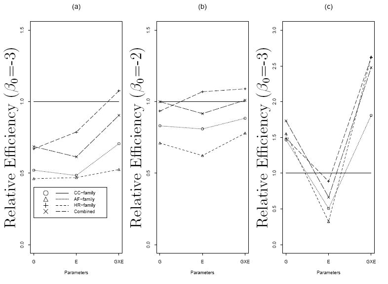
Relative efficiencies of different study designs by baseline log odds β₀ and allele frequency p. Panel (a): p = 0.1 and logit(Pr(D = 1∣G,E)) = −3 + log(1.5)G + log(2)E + log(3)G × E; Panel (b): p = 0.1 and logit(Pr(D = 1∣G,E)) = −2 + log(1.5)G + log(2)E + log(3)G × E; Panel (c): p = 0.01 and logit(Pr(D = 1∣G,E)) = −3 + log(15)G + log(2)E + log(10)G × E. The solid horizontal lines represent the relative efficiency for population based case-control studies.

4. An Example from a Study of Colorectal Cancer

Strong evidence of familial aggregation has been established in Colorectal cancer (CRC). Based on studies of high risk families, several genetic factors contributing to CRC susceptibility have been identified, including a mutation in the APC gene for familial adenomatous polyposis (FAP), and a mutation in the DNA mismatch repair (MMR) genes for hereditary nonpolyposis colorectal cancer (HNPCC) (Peltomaki and Vasen, 1997). Currently a multi-stage genome-wide association study is being carried out using Colon CFR resources, and the variants identified from such a study will be assessed for disease association by studying cases, unrelated controls and family members enrolled in the Colon CFR. It is valuable to further characterize these loci, especially their joint effects with modifiable lifestyle and environmental factors, such as smoking, physical activity and diet, as such an evaluation will have considerable clinical importance in colorectal cancer prevention.

To illustrate the proposed method, we analyzed data from the Fred Hutchinson Cancer Research Center, one of the six study sites in Colon CFR. Details regarding case and control eligibility, recruitment, data and specimen collection have been reported previously in Newcomb et al. (2007). We focus here on evaluating the main effects of smoking and body mass index (BMI) on CRC risk, as this is an important initial step toward our future analysis of modifiers of genetic risk in CRC in this study population. In the dataset we have baseline epidemiologic risk factors collected on 1905 incident CRC cases who were diagnosed between 1998 and 2002 and between the ages of 20 and 74 years, and 2302 unrelated controls identified from the same catchment area. Cases reported their smoking history and other exposure information in the year prior to diagnosis and controls during a similar reference period. In addition, 5296 first degree relatives of 1627 case probands were recruited. The median family size (including the proband) was 3. Among these, 1129 case probands had epidemiologic information available on their siblings, with 2229 sib-controls.

A logistic regression model was used to assess the effects of smoking (never, former, current) and BMI (kg/m² in quartiles), adjusting for age (in 10-year intervals), gender and colorectal screening sigmoidoscopy history within the past 10 years (yes, no, unknown). In the analysis that consists of cases and unrelated controls, compared to individuals who never smoke, there was a statistically significant increase in CRC risk among former smokers (OR=1.199, 95% confidence interval (CI) [1.045-1.376]), and particularly among the current smokers (OR=1.653, 95% CI [1.375-1.987]). The trend is consistent with that reported in the literature (Giovannucci, 2001). Increased risks were also observed in individuals with higher levels of BMI (Table 3). None of these effects were significant, however, when we restricted the analysis to only case probands and their siblings and when using the conventional conditional logistic regression model. Expanding family data to include both parents and offspring in addition to siblings yielded significant effects of smoking and BMI with the conditional logistic regression model, though the magnitude of odds ratios tended to be higher than that from the case-unrelated control study for most of the scenarios. Combining cases, siblings and unrelated controls, using the method proposed in Section 2, again yielded significant effects of smoking and BMI. The magnitude of OR estimates in this case was very close to those from the analysis using cases and unrelated controls, although with improved efficiency. Similar results were obtained when we considered data from all available family members and unrelated controls, although the estimates for σ in the family-specific random effect differed.

Table 3.

Odds ratios (estimate (95% confidence interval), relative efficiency^*) of the association between CRC risk and smoke and BMI, by type of models and type of subjects included in the model. CC: ordinal logistic regression model with population-based case and control data; CL: Conditional logistic regression model for family data; Combined: ascertainment adjusted marginalized logistic-normal model. All model adjusted for age, gender and screening history.

Model	Cases (freq.)	Controls (freq.)	Family (freq.)	Smoking		BMI
				Former vs. Never	Current vs. Never	BMI2 vs. BMI1	BMI3 vs. BMI1	BMI4 vs. BMI1
CC	1950	2302	4252	1.20 (1.05–1.38) 1.00	1.65 (1.38–1.99) 1.00	1.16 (0.96–1.40) 1.00	1.33 (1.10–1.59) 1.00	1.75 (1.46–2.11) 1.00
All Siblings
CL	1129	2229	1129	1.06 (0.87–1.29) 0.54	0.92 (0.72–1.18) 0.93	1.09 (0.85–1.39) 0.58	1.16 (0.90–1.49) 0.56	1.32 (1.01–1.73) 0.59
Combined†	2302	4179	4252	1.19 (1.04–1.36) 1.06	1.53 (1.28–1.83) 1.15	1.14 (0.95–1.36) 1.08	1.31 (1.10–1.57) 1.08	1.70 (1.41–2.03) 1.11
All Family Members
CL	1627	5296	1627	1.30 (1.12–1.50) 0.83	1.22 (1.01–1.47) 1.33	1.27 (1.05–1.53) 0.90	1.48 (1.22–1.78) 0.84	1.77 (1.45–2.16) 0.83
Combined‡	2302	7246	4252	1.18 (1.04–1.34) 1.30	1.49 (1.26–1.77) 1.30	1.13 (0.95–1.35) 1.16	1.31 (1.10–1.56) 1.15	1.69 (1.42–2.02) 1.19

^*: Relative efficiency is defined as the ratio of the normalized variance (variance/estimate) for CC versus normalized variance for the design

^†: σ = 1.64 (0.82–3.31)

^‡: σ = 0.53 (0.12–2.45)

In Table 3 we also list the estimates of relative efficiencies for different sets of data compared with the variance from the case and unrelated control data.Combining data always yields better efficiency, compared with analysis using population based control only, especially in the case where information from all family members was considered. The increase in efficiency is moderate however, ranging from 6% to 33%, indicating that the bulk of information on covariate effects still comes from the population-based case-control data.

5. Discussion

Large association studies that collect data at both population and family levels have been conducted for certain diseases. As in the case of Colon CFR study, such a design is valuable as it permits the evaluation of a broad spectrum of allele frequencies and exposures. We have described a general approach to combining data from both a family-based study and a case-unrelated control study to increase the power to detect an association in this setting. To specify the likelihood for data from a family study, we adopt a marginalized mixed effect model which was previously proposed for longitudinal data (Heagerty, 1999). The model allows us to account for residual correlations among family members naturally by using a family-specific random effect model, while specifying regression parameters at population level. The likelihood contribution from a family is conditioned on the ascertainment event to allow for retrospective case-control family study designs or other types of outcome dependent sampling in family studies. The likelihood contributions from the case-control and family studies can then be combined, and MLEs are found from the joint likelihood function. The proposed estimators are asymptotically unbiased for marginal covariate effects and are more efficient than an estimating equation-based method.

The proposed method is related to other work in the family study literature. Pfeiffer et al. (2008) considered a two-level random effects model for family data and conditioned the likelihood on the event that at least two diseased members are sampled in each family. Similar conditional prospective likelihood was also described in Kraft and Thomas (2000). Similarly we also used a generalised linear mixed model to characterize the correlations within a family. However our methods differ from these other proposals in that we base our inference at the population level, whereas parameters from these other models are conditional on the unobserved family-specific random effects. Our model will be useful for studies that aim to characterize the averaged covariate effects on disease risk in the population. For family designs involving outcome dependent sampling, we used ascertainment-adjusted likelihood, which requires an explicit modeling of the ascertainment events. Other authors considered semiparametric likelihood approaches to accommodate sampling. Neuhaus et al. (2002) proposed to divide the population of families into strata defined by the disease outcomes in a family, and made inference based on the full joint likelihood of the strata; whereas Pfeiffer et al. (2008) proposed similar stratification based on case control status and family history with a weighted estimating equation approach for estimation. The former requires that families be categorized into distinct groups and the latter needs non-zero sampling probabilities for the strata. Our approach does not have such limitations.

There are caveats when applying our proposed procedures. First, since we employed fully parametric models for family data, there is potential for model misspecification. In general, estimates of fixed effects from a mixed model are not sensitive to the misspecification of the underlying distribution of random effects, however biased estimates can result if the random effects are dependent on covariates (Heagerty and Kurland, 2001). By allowing family-level random effects to vary with covariates, our procedure can be quite flexible. Second, unlike the conditional logistic regression where nuisance parameters (family-specific intercepts) are conditioned out of the likelihood, the conditional prospective likelihood approach explicitly estimates baseline risk and random effect parameters. While such a model appears to be asymptotically identifiable, it does not ensure convergence for a given finite sample. For example, in finite samples with rare disease and the family-based ascertainment scheme we may not have sufficient information on β₀ and σ. This problem manifests in numerical instability of standard optimization procedures, especially when applied with only family data. Our experience with simulation studies shows that the rate of successful numerical convergence generally decrease for association models that have lower values of the intercept term. This problem may be alleviated by bringing in additional information such as baseline risk estimated from the entire population as in Neuhaus et al. (2006), or using a grid-search algorithm as suggested by Pfeiffer et al. (2001). Third, we have made the key assumption that ORs are homogeneous in case-unrelated controls and case-relatives. However, potential sources of genuine heterogeneity can yield different estimates from the two sources of data. For example, population substructure may cause spurious associations between genetic polymorphisms and disease risk from a population-based study. Additional simulation studies (not show) explored unmeasured heterogeneity, or population stratification, and suggest that our proposed methods will be biased without an adjustment for subpopulation membership because in this case the marginal model is misspecified. Therefore, in practice we do not recommend use of our methods for combining data if there is evidence of heterogeneity. However if there are additional measured genetic markers or variables reflective of subpopulation membership then the impact of population stratification can be minimized by adjusting for these markers. In our application of Colon CFR data, population stratification is unlikely to be a source of heterogeneity.

References

- Anderson J. Separate sample logistic discrimination. Biometrika. 1972;59:19–35. [Google Scholar]
- Bahadur RR. A representation of the joint distribution of responses to n dichoomous outcomes. Studies in item analysis and prediction. Standford University Press; 1999. [Google Scholar]
- Breslow N, Day N. Statistical Methods in Cancer Research (Vol.1): The Analysis of Case-control Studies. IARC Scientific Publications; New York: 1980. [PubMed] [Google Scholar]
- Chen Y, Lin H. Simple association analysis combing data from trios/sibships and unrelated controls. Genetic Epidemiology. 2008;32:520–527. doi: 10.1002/gepi.20325. [DOI] [PubMed] [Google Scholar]
- Giovannucci E. An updated review of the epidemiological evidence that cigarette smoking increases risk of colorectal cancer. Cancer epidimiology, Biomarkers and Prevention. 2001;10:725–731. [PubMed] [Google Scholar]
- Heagerty PJ. Marginally specified logistic-normal models for longitudinal binary data. Biometrics. 1999;55:688–698. doi: 10.1111/j.0006-341x.1999.00688.x. [DOI] [PubMed] [Google Scholar]
- Heagerty PJ, Kurland BF. Misspecified maximum likelihood estimates and generalised linear mixed models. Biometrika. 2001;88:973–985. [Google Scholar]
- Heagerty PJ, Zeger SL. Marginalized multilevel models and likelihood inference (with comments and a rejoinder by the authors) Statistical Science. 2000;15:1–26. [Google Scholar]
- Kraft P, Thomas D. Bias and efficiency in family-based gene-characterization studies: conditional, prospective, retrospecti ve and joint likelihoods. American Journal of Human Genetics. 2000;66:1119–1131. doi: 10.1086/302808. [DOI] [PMC free article] [PubMed] [Google Scholar]
- Landi M, Kanetsky P, Tsang S, et al. MC1R, ASIP, and DNA Repair in sporadic and familial melanoma in a mediterranean population. JNCI. 2005;97:998–1007. doi: 10.1093/jnci/dji176. [DOI] [PubMed] [Google Scholar]
- Neuhaus J, Scott A, Wild C. The analysis of retrospective family studies. Biometrika. 2002;89:23–37. [Google Scholar]
- Neuhaus JM, Scott AJ, Wild CJ. Family-specific approaches to the analysis of case-control family data. Biometrics. 2006;62:488–494. doi: 10.1111/j.1541-0420.2005.00450.x. [DOI] [PubMed] [Google Scholar]
- Newcomb P, Baron J, Cotterchio M, Gallinger, et al. Colon cancer family registry: An international resource for studies of the genetic epidemiology of colon cancer. Cancer Epidemiology, Biomarkers, Prevention. 2007;16:2331–2343. doi: 10.1158/1055-9965.EPI-07-0648. [DOI] [PubMed] [Google Scholar]
- Peltomaki P, Vasen H. The International Collaborative Group on Hereditary Nonpolyposis Colorectal Cancer. Mutations predisposing to hereditary nonpolyposis colorectal ancer; database and results of a collaborative study. Gastroenterology. 1997;113:1146–58. doi: 10.1053/gast.1997.v113.pm9322509. [DOI] [PubMed] [Google Scholar]
- Pfeiffer RM, Gail MH, Pee D. Inference for covariates that accounts for ascertainment and random genetic effects in family studies. Biometrika. 2001;88:933–948. [Google Scholar]
- Pfeiffer RM, Pee D, Landi MT. On combining family and case-control studies. Genetic Epidemiology. 2008;32:638–46. doi: 10.1002/gepi.20338. [DOI] [PMC free article] [PubMed] [Google Scholar]
- Prentice RL. Correlated binary regression with covariates specific to each binary observation. Biometrics. 1988;44:1033–1048. [PubMed] [Google Scholar]
- Prentice RL, Pyke R. Logistic disease incidence models and case-control studies. Biometrika. 1979;66:403–412. [Google Scholar]
- Slager S, Schaid D. Evaluation of candidate genes in case-control studies: A statistical method to account for related subjects. American Journal of Human Genetics. 2001;68:1457–1462. doi: 10.1086/320608. [DOI] [PMC free article] [PubMed] [Google Scholar]
- Thornton T, McPeek M. Case-control association testing with related individuals: A more powerful quasi-likelihood score test. American Journal of Human Genetics. 2007;81:321–337. doi: 10.1086/519497. [DOI] [PMC free article] [PubMed] [Google Scholar]
- Whittemore A, Halpern J. Logistic regression of family data from retrospective study designs. American Journal of Human Genetics. 2003;81:321–337. doi: 10.1002/gepi.10267. [DOI] [PubMed] [Google Scholar]
- Whittemore AS. Logistic regression of family data from case-control studies (Corr: 97V84 p989-990) Biometrika. 1995;82:57–67. [Google Scholar]
- Witte J, Gauderman W, Thomas D. Asymptotic bias and efficiency in case-control studies of candidate genes and gene-environment interactions: Basic family designs. Am J Epidem. 1999;149:693–705. doi: 10.1093/oxfordjournals.aje.a009877. [DOI] [PubMed] [Google Scholar]
- Zeger S, Liang K, Albert P. Models for longitudinal data: A generalized estimating equation approach. Biometrics. 1988;44:1049–1060. [PubMed] [Google Scholar]
- Zhao LP, Hsu L, Holte S, Chen Y, Quiaoit F, Prentice RL. Combined association and aggregation analysis of data from case-control family studies. Biometrika. 1998;85:299–315. [Google Scholar]