Improving Marginal Likelihood Estimation for Bayesian Phylogenetic Model Selection

Abstract

The marginal likelihood is commonly used for comparing different evolutionary models in Bayesian phylogenetics and is the central quantity used in computing Bayes Factors for comparing model fit. A popular method for estimating marginal likelihoods, the harmonic mean (HM) method, can be easily computed from the output of a Markov chain Monte Carlo analysis but often greatly overestimates the marginal likelihood. The thermodynamic integration (TI) method is much more accurate than the HM method but requires more computation. In this paper, we introduce a new method, steppingstone sampling (SS), which uses importance sampling to estimate each ratio in a series (the “stepping stones”) bridging the posterior and prior distributions. We compare the performance of the SS approach to the TI and HM methods in simulation and using real data. We conclude that the greatly increased accuracy of the SS and TI methods argues for their use instead of the HM method, despite the extra computation needed.

The application of Bayesian statistics to phylogenetics (Rannala and Yang 1996, Mau and Newton 1997, Yang and Rannala 1997, Larget and Simon 1999, Newton et al. 1999, Li et al. 2000, Drummond et al. 2002) introduced not only a new way of estimating phylogenies but also new ways of evaluating models used for phylogenetic inference. For example, the Bayes factor is a ratio of the marginal likelihood of one model to the marginal likelihood of a competing model. The marginal likelihood measures the average fit of a model to the data, whereas traditional approaches to model selection, such as likelihood ratio tests (LRT; Wilks 1938), the Akaike Information Criterion (AIC; Akaike 1974), the Bayesian Information Criterion (BIC; Schwarz 1978), and the decision-theoretic approach (DT; Minin et al. 2003), base decisions on the fit of each competing model at its best (i.e. the point in parameter space that maximizes the likelihood). Despite the name, the BIC does not take account of the priors that are actually used in a Bayesian analysis, and the same is true of the other non-Bayesian approaches (AIC, LRT, and DT).

There are two primary reasons as to why taking the prior into account is important in Bayesian model selection. First, if the prior is informative, it may “box out” a parameter, keeping the parameter from attaining values that would provide the best fit to the data. A prior distribution has the effect of attaching a metaphorical rubber band to a parameter value. The variance of a prior distribution measures the average strength of its rubber band, and the prior mode specifies where the rubber band is staked to the ground. For vague relatively noninformative priors (large variance), the rubber band is very thin and stretches easily, allowing the parameter to take on essentially any value suggested by the data. Informative priors (small variance) attach thick strong rubber bands to their parameters, keeping the parameter value relatively close to the prior mode. Making the prior informative and at the same time staking it down too far away from the zone of best fit will prevent the model from fitting the data well in a Bayesian analysis. Because LRT, AIC, BIC, and DT ignore priors, these approaches to model selection will not detect that the prior is preventing the model from fitting the data well. Most priors currently utilized in Bayesian phylogenetic analyses are vague and the models used are not overly complex. As models become more biologically realistic, more parameter-rich informative priors will be needed for at least some parameters to avoid overparameterization, and “boxing out” will become more of a concern.

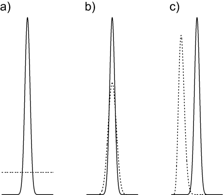
The second reason why priors are important in Bayesian model selection lies in the fact that it is the prior that determines the degree to which an extra parameter in overly complex models is penalized when the marginal likelihood is used to assess model performance. All model choice criteria reward models for high goodness-of-fit and penalize models for gratuitous complexity. AIC and BIC both punish unnecessarily complex models by assessing a penalty for each parameter. If adding a parameter does not increase the maximized likelihood enough to offset the penalty, the model will not be favored when compared to a model lacking that parameter. The penalty term is the same for every parameter in AIC and BIC. For example, the Hasegawa–Kishino–Yano (HKY)+G model is penalized just as much by AIC and BIC for having a discrete gamma rate heterogeneity shape parameter as it is for having a transition/transversion rate ratio parameter. On the other hand, Bayesian model selection using the Bayes Factor (BF) approach allows the investigator to specify an individual penalty for each parameter through the choice of prior distributions. The marginal likelihood is a weighted average of the likelihood, where the weights come from the prior. The marginal likelihood is highest when the prior and likelihood are both concentrated over the same parameter value regions, and the marginal likelihood of a model is lowest when the prior emphasizes regions of parameter space where the likelihood is low. Choosing a prior that is both informative and in accordance with the likelihood (Fig. 1b) will penalize a model less than a prior that is either noninformative (Fig. 1a) or informative but with little overlap with the likelihood (Fig. 1c). BFs thus provide tunable penalties for parameters in models, whereas the traditional approaches treat parameters equally.

Calculating the marginal likelihood of a model exactly is computationally intractable for all but trivial phylogenetic models. The marginal likelihood must therefore be approximated using Markov chain Monte Carlo (MCMC), making Bayesian model selection using BFs time consuming compared with the use of LRT, AIC, BIC, and DT for model selection. For nested models (one model is a special case of the other model), BFs can be estimated using the Savage-Dickey ratio (Suchard et al. 2001); however, many interesting model comparisons involve nonnested models. Huelsenbeck et al. (2004) used reversible-jump MCMC (rjMCMC) to perform model averaging over the entire family of models that represent various constrained versions of the general time reversible (GTR) model. This approach indirectly uses marginal likelihoods as model weights, avoiding the technical difficulties associated with marginal likelihood estimation while at the same time also avoiding model choice. The disadvantage of the rjMCMC approach is that it is restricted to a specific fixed family of models; adding a new model would be tedious, requiring design of an ad hoc MCMC proposal that allows jumps between the new model and at least one other model already in the system. Because of its ease of calculation, the harmonic mean (HM) approach (Newton and Raftery 1994) is the most common approach for estimating marginal likelihoods, and hence BFs (e.g., Nylander et al. 2004, Pagel and Meade 2004, Brandley et al. 2005, Bleidorn et al. 2007, Brown and Lemmon 2007, Alekseyenko et al. 2008, Praz et al. 2008). Lartillot and Philippe (2006) advocated thermodynamic integration (TI) for estimating the marginal likelihood of a single model (the “annealing-melting integration” variant) or the BF directly (the “model-switch integration” variant). The TI approach is far more accurate than the HM method, but requires an MCMC analysis that is more time consuming than that needed by the HM method.

This paper is concerned with describing a new method (steppingstone sampling; SS) that provides an alternative to TI. As with the annealing-melting version of TI, SS estimates the marginal likelihood directly as opposed to estimating a ratio of marginal likelihoods (i.e., BF). This makes these two methods very general: they can be applied to any model for which MCMC samples can be obtained. Direct estimation of marginal likelihoods allows a new model to be compared with published marginal likelihoods of other models, which is impossible for methods that estimate BFs directly unless a common reference model is used. A further limitation of methods that directly estimate BFs arises if the models being compared occupy different parameter spaces, a situation that requires special treatment on a case-by-case basis (Chen and Shao 1997). We present simulation results showing that (because of its increased accuracy) the SS method often chooses different models than the HM method, and results from empirical examples showing that SS and TI provide very similar estimates of the marginal likelihood. We conclude that the HM method is quite inferior to both SS and TI and should not be used for model choice in phylogenetics if these alternatives are available.

MARGINAL LIKELIHOOD ESTIMATION

Importance-Sampling Approaches

An approximation to the marginal likelihood can be obtained by importance sampling. Allowing an MCMC sampler to explore the importance distribution g(θ), the marginal likelihood can be estimated using the sampled θ_i values (i = 1,…,n) as follows:

(1)

where θ_i represents the ith parameter vector sampled from the importance distribution, f(y|θ_i,M) is the likelihood computed at point θ_i, and w(θ_i|M) is the importance weight for observation i. The weight w(θ_i|M) in turn equals f(θ_i|M)/g(θ_i), where f(θ_i|M) is the joint prior density computed at point θ_i and g(θ_i) is the importance density computed at point θ_i.

The difference between different importance-sampling estimators lies in the choice of the importance distribution. The posterior distribution f(θ|y,M) is a particularly convenient choice for g(θ) because a sample from the posterior is the goal of any Bayesian phylogenetic analysis, allowing the marginal likelihood to be estimated from an MCMC sample that must be collected anyway. Equating g(θ) with the posterior distribution means that an estimate of the marginal likelihood can be obtained essentially for free. Substituting g(θ) = f(θ|y,M) = f(y|θ,M)f(θ|M)/f(y|M) into Equation 1 shows that the estimate of the marginal likelihood under this choice for g(θ) is the HM of the likelihoods sampled from the posterior distribution:

This importance-sampling approach for approximating the marginal likelihood was introduced by Newton and Raftery (1994) and is known as the harmonic mean (HM) method. The HM method is currently very popular, largely because widely used computer programs such as MrBayes (Ronquist and Huelsenbeck 2003) provide the log HM as part of their standard output. Unfortunately, the HM estimator is biased and overestimates the true marginal likelihood (Appendix). Intuitively, this overestimation is easy to understand in the (usual) case of a diffuse prior and a posterior dominated by the likelihood. In such cases, few MCMC samples will come from areas of parameter space in which the likelihood is low, even if such areas are not discouraged by the prior, leading to an overrepresentation of high likelihoods in the estimate of marginal likelihood.

The arithmetic mean (AM) method uses the prior as the importance distribution. Substituting g(θ) = f(θ|M) into Equation 1, the marginal likelihood estimate is the simple AM of the likelihoods sampled from the prior distribution. This approach is unbiased; however, if the likelihood is sharp compared with the prior, the AM estimate can have an unacceptably high variance. This is because the magnitude of the estimate often depends critically on a few points sampled in the area of high likelihood. As we show later, the AM method becomes very useful when the importance distribution is chosen to be similar to (but slightly broader than) the target distribution.

Thermodynamic Integration

The most accurate method currently used in phylogenetics to estimate marginal likelihoods is not an importance-sampling approach. This method, TI, is similar to the path sampling method of Gelman and Meng (1998) and was first introduced into phylogenetics by Lartillot and Philippe (2006). Apparently unaware of Lartillot and Philippe (2006), Friel and Pettitt (2008) arrived at the same method independently (but did not apply it to phylogenetics), calling it the method of power posteriors. Lartillot and Philippe (2006) showed that TI is far more accurate than HM.

TI avoids the overestimation of HM by sampling from a Markov chain that explores a near-continuous progression of distributions along a path extending from the posterior at one extreme to the prior at the other extreme. Lartillot and Philippe (2006) termed this “annealing-melting integration.” The other form of TI they described, “model-switch integration,” involves following a path between the posterior distributions of two separate models. The method outlined by Lartillot and Philippe (2006) and Friel and Pettitt (2008) differs from the path sampling method defined by Gelman and Meng (1998). In Gelman and Meng's approach, points along the path from prior to posterior are drawn from a probability distribution. This works well in a pure Gibbs-sampling context where no burn-in period is required; however, in phylogenetics, where Metropolis-within-Gibbs sampling dominates, this approach is very inefficient due to the need to allow the chain to acclimate to potentially radical shifts in the target distribution. In the method of Lartillot and Philippe (2006), the sampler crawls incrementally along the path between the prior and posterior, and the time spent sampling one point along the path serves as the burn-in period for sampling the next point.

Lartillot and Philippe (2006) discuss discretization error, which is a form of bias that causes underestimation of the marginal likelihood. Discretization bias arises because the method approximates a continuous integral using a finite number of points. The bias decreases with the number of points composing the path (it cannot be ameliorated by devoting more sampling effort to each point). Discretization bias becomes an issue only when one attempts to cut corners by using a small number of intervals along the path. The primary practical difficulty with TI is thus the amount of computation required to be assured that this inherent bias is negligible. Lartillot and Philippe (2006) predicted that TI may require an order of magnitude more computation than would be required for obtaining an adequate sample from the posterior distribution for purposes of parameter estimation.

In the next section, we introduce a new method, SS, that lacks discretization bias and is slightly less computationally costly than TI. SS combines elements of both TI and importance sampling. We later compare the performance of SS to TI and HM in simulation and in analyses of real data.

METHODS

Steppingstone Sampling

Consider the unnormalized power posterior density function q_β(θ), which has normalizing constant c_β, yielding the normalized power posterior density p_β:

where f(y|θ,M) is the likelihood function and f(θ|M) the prior. The power posterior is equivalent to the posterior distribution when β = 1.0 and is equivalent to the prior distribution when β = 0.0. The goal is to estimate the ratio c_1.0/c_0.0, which is equivalent to the marginal likelihood because c_0.0 = 1.0 if the prior is proper (which is assumed throughout). Note that this ratio can be expressed as a product of K ratios:

where β_k = k/K,k = 1,2,…,K. The basic idea of SS is to estimate each ratio c_βk/c_{βk − 1} in the product by importance sampling, using p_{βk − 1} as the importance-sampling density. Because (for K large) p_{βk − 1} is only slightly more dispersed than p_βk, it serves as an excellent importance distribution (Chen et al. 2000, p. 134). Utilizing the importance-sampling formula (Equation 1) to approximate both the numerator, f(y|M,β_k), and denominator, f(y|M,β_{k − 1}), of the desired ratio (r_SS,k) of marginal likelihoods, and assuming g = p_{βk − 1},

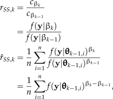where θ_{k − 1,i} is an MCMC sample from p_{βk − 1} and f(y|θ_{k − 1,i}) is the likelihood of that sampled parameter vector. Dependence of all likelihoods and priors on the model under consideration (M) has been suppressed in the notation for simplicity. Note that this method reduces to the AM method for the special case K = 1. Interestingly, with SS, there is no need to sample the posterior; however, in practice, we use an initial exploration of the posterior as a means of burning-in the MCMC sampler.

Numerical stability can be improved by factoring out the largest sampled likelihood term, L_max,k = max_{1 ≤ i ≤ n}f(y|θ_{k − 1,i}):

Combining all K ratios, the SS estimate of the marginal likelihood is simply

Being a product of independent unbiased estimators, is itself unbiased. On the log scale,

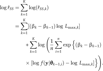Although is unbiased, changing to the log scale introduces a bias. This bias appears to be directly proportional to the variance of log(), which can be alleviated by increasing K. The lognormal distribution provides an analogy. If log(X) is normal with mean μ and variance σ², then logE[X] = μ + σ²/2, which is larger than E[log(X)] by an amount proportional to the variance of log(X). Similarly, the mean of the log-marginal likelihood estimated by SS is smaller than the true value by an amount proportional to the variance on the log scale. The simulation variance of _,k is estimated by

Based on the δ method (Oehlert 1992), the variance of is approximated by:

A Better Path

In TI, an MCMC sample is drawn from a series of K + 1 distributions, each of which is a power posterior differing only in the power β:

Lartillot and Philippe (2006) advocated spreading the K + 1 values of β evenly from 0.0 to 1.0. Lepage et al. (2007) used a sigmoidal function that placed most β values near the extremes of the unit interval in their model-switch TI analysis. Friel and Pettitt (2008) chose β_k = a_k⁴, where the a = 0.0,0.1,…,1.0. The Lepage et al. (2007) and Friel and Pettitt (2008) approaches both place most of the β values at points where the power posterior is changing rapidly. In the common situation where the likelihood is much more concentrated than the prior, the shape of the power posterior is relatively stable except near β = 0, so placing more computational effort near 0 is sensible and (as we later show) leads to a substantial increase in the efficiency of the estimator, where better efficiency is defined as the same accuracy with fewer values of β. We chose to use a Beta(α, 1.0) distribution to select values of β. Specifically, choosing β_k = (k/K)^1/α selects β values according to evenly spaced quantiles of the Beta(α, 1.0) distribution, placing most values of β near 0 (in fact, Friel and Pettitt's method represents the special case α = 0.25). The value of α is inversely related to skewness: when α = 1.0, β values are uniformly spaced from 0.0 to 1.0; however, when (for example) α = 0.3, the Beta(α,1.0) distribution is positively skewed such that half of the β values are less than 0.1. We investigated the effect of the choice of α on the efficiency of TI and SS.

EXAMPLES

Standard Normal Example

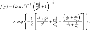
A comparison of methods using normal distributions is instructive because of the fact that the true value of the marginal likelihood is available analytically and direct draws from the posterior avoid any complications due to MCMC approximation. Suppose n observations are sampled from a normal distribution having mean μ and standard deviation τ,

and define

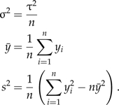Letting the prior on μ be normal with mean μ₀ and standard deviation σ₀, the power posterior of μ (conditioned on σ) is as follows:

and the marginal likelihood is

(2)

We performed a simulation experiment to compare the performance of the HM, TI, and SS methods. A single data set of size n = 100 was simulated from a normal distribution having mean μ = 0.0 and standard deviation τ = 1.0. The simulated data set is available in the Supplementary Material (available from http://www.sysbio.oxfordjournals.org). We sampled 2000 values of μ directly from each power posterior, p_β, using K + 1 values of β either spaced uniformly along the path from β = 0.0 to β = 1.0, or according to uniformly spaced quantiles of a Beta(α, 1.0) distribution. HM analyses were based on 2000(K + 1) posterior samples so that HM was allotted the same computational effort as TI. SS was at a slight disadvantage because it uses samples from only K distributions. The prior for μ was normal with mean μ₀ = 0.0 and standard deviation σ₀ = 1.0.

Using Equation 2, the natural logarithm of the true marginal likelihood was log(c₁) = − 147.916. To assess accuracy, we computed the root mean square error (RMSE) over 1000 independent MCMC analyses using each of the three methods. The RMSE is defined as

Note that the mean square error can be decomposed into a variance term, , plus a bias term, . Thus, for an unbiased method the RMSE equals the standard error, .

Three generalizations are suggested by the simulation results in the standard normal example (Table 1), regardless of the number of β intervals used (K = 50 vs. K = 100) or the distribution of the β values (uniform vs. Beta(0.3,1.0)). First, TI and SS do much better than HM at estimating the marginal likelihood. Based on the best RMSE for each method, SS was the best method (RMSE = 0.0074) followed closely by TI (RMSE = 0.0079), with HM a distant last (RMSE = 0.9479). HM thus performed 128 times worse than SS, and 120 times worse than TI. As expected, HM substantially overestimated the marginal likelihood, making the model appear better-fitting than it really was. Second, comparing SE to RMSE shows that TI is biased (although not nearly as much as HM), whereas SS is evidently unbiased. Third, using a Beta distribution favoring small values of β greatly improves the performance of all methods except HM, for which β is irrelevant.

Table 1.

Results from analysis of standard normal data

Uniform path for βa
Method	Kb = 100			K = 50
	Mean	SEc	RMSEd	Mean	SE	RMSE
HMe	–147.020	0.3081	0.9479	–146.991	0.3179	0.9779
TIf	–147.955	0.0146	0.0413	–148.053	0.0218	0.1384
SSg	–147.916	0.0135	0.0135	–147.916	0.0162	0.0162
Beta(0.3,1) path for β
Method	K = 100			K = 50
	Mean	SE	RMSE	Mean	SE	RMSE
HM	–147.020	0.3081	0.9479	–146.991	0.3179	0.9779
TI	–147.917	0.0078	0.0079	–147.921	0.0115	0.0123
SS	–147.916	0.0074	0.0074	–147.916	0.0105	0.0105

^aThe power to which the likelihood is raised in the power posterior distribution.

^bThe number of β intervals.

^cStandard error.

^dRoot mean square error.

^eHarmonic mean method.

^fThermodynamic integration method.

^gSteppingstone method.

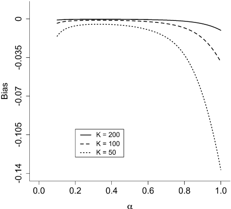
Figure 2 shows the bias in TI as a function of the parameter α (the shape parameter of the Beta distribution used to determine β values) and K (the number of β intervals). The bias is always negative, indicating that TI tends to underestimate the marginal likelihood, and gets worse with smaller values of K. For this example, there is an optimum value of α between 0.2 and 0.4 that minimizes the bias for any value of K. Lartillot and Philippe (2006) discuss two forms of bias in TI: thermic lag bias and discretization bias. Thermic lag bias results from the fact that when the value of β is switched, the Markov chain takes some time to adjust to the new value. This thermic lag causes underestimation of the marginal likelihood if β values begin at 0.0 and progress toward 1.0, and overestimation if the first β value is 1.0 and the progression is toward 0.0. Our results, however, are based on direct sampling from the full conditional power posterior distribution, so the bias in this case is entirely discretization bias.

FIGURE 2.

Bias of the TI method for different numbers and distributions of β values in the standard normal example. K is the number of β intervals, and β values are evenly spaced quantiles from a Beta(α,1.0) distribution. Bias is defined as .

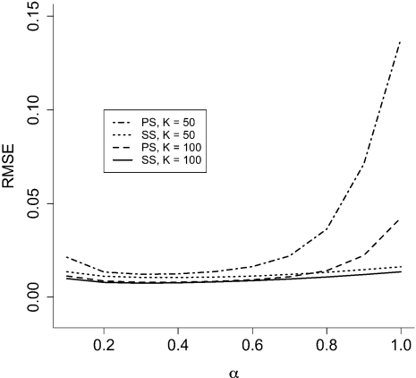
Figure 3 shows the RMSE of TI and SS estimates of the marginal likelihood as a function of α and K. Both methods perform best when the distribution of β values is moderately positively skewed (i.e., α between 0.2 and 0.4), and both perform better with more β values (i.e., K larger). SS is more efficient than TI for any combination of K and α, but the difference between these two methods is small compared with the considerable improvement found for both SS and TI when switching from even to skewed spacing of β values. For example, setting α = 0.3 (instead of α = 1.0) achieves 3.5 times (TI) or 1.3 times (SS) better accuracy with less than half the computational effort (K = 50 vs. K = 100).

FIGURE 3.

RMSE of the TI and SS methods for different numbers and distributions of β values in the standard normal example. K is the number of β intervals, and β values are evenly spaced quantiles from a Beta(α,1.0) distribution.

Green Plant rbcL Example

Methods for estimating marginal likelihoods should be sensitive to priors. Specifically, decreasing the informativeness of a prior distribution for one or more parameters of a model typically increases the contribution of low-likelihood regions of parameter space to the true marginal likelihood, and this should be reflected in the estimated marginal likelihood. Because HM tends to ignore regions of parameter space where the likelihood is low, we hypothesized that the HM method would be less sensitive to priors than the TI or SS methods. This aspect of the estimation methods can be investigated even for the (usual) situation in which we do not know the true marginal likelihood.

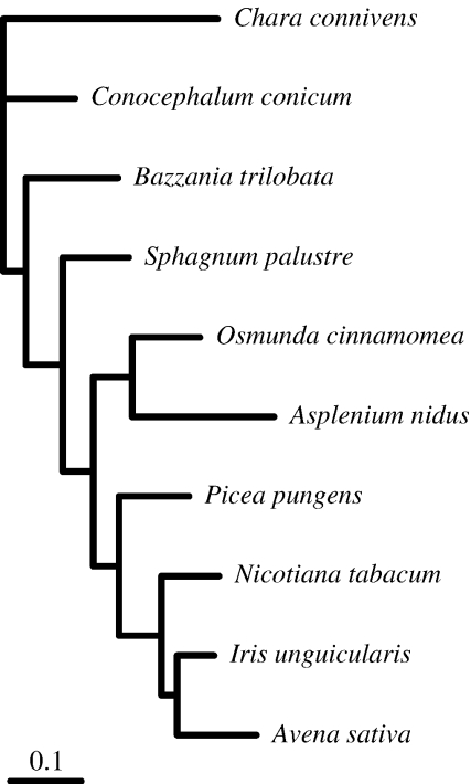
We analyzed a 10-taxon green plant data set using DNA sequences of the chloroplast-encoded large subunit of the RuBisCO gene (rbcL). Taxa were chosen arbitrarily for this example, but with the intent to sample broadly across green plants. The alignment and GenBank accession numbers are provided in the Supplementary Material. The phylogeny for these 10 taxa is uncontroversial: the same tree topology (Fig. 4) is obtained using any standard model of DNA sequence evolution as long as transition/transversion bias and among-site rate heterogeneity are accommodated.

FIGURE 4.

The topology assumed for the green plant rbcL example. The tree topology and branch lengths were estimated by maximum likelihood using the GTR+G model.

In order to investigate the sensitivity of methods to prior distributions, we estimated the marginal likelihood using three methods (HM, TI, and SS) under the HKY85+G model and three different prior distributions. The models differed only in the prior placed on the discrete gamma among-site rate heterogeneity shape parameter. The three priors are Exponential(0.001) (nicknamed the “vague” prior), Gamma(10,0.026) (the “good” prior), and Gamma(148, 0.00676) (the “wrong” prior). It is impossible to place a prior that is both flat and proper on an unbounded parameter, but the “vague” prior has variance 1 million, which makes it much less informative than the “good” or “wrong” priors. The “good” and “wrong” priors have the same variance, but differ in their means, with the mean of the “good” prior centered around the posterior mean based on preliminary runs, and the mean of the `wrong” prior set (arbitrarily) to 1.0. This choice of priors mimics those depicted in Figure 1, with Figure 1a corresponding to “vague”, Figure 1b to “good” and Figure 1c to “wrong”. We recognize that no prior can really be considered wrong as long as it reflects the beliefs of the investigator, so we use the nickname “wrong” here solely to denote the fact that the data strongly contradict this prior.

FIGURE 1.

Three possible priors (dotted lines) for an analysis in which the likelihood is indicated by a solid line. a) Flat prior. b) Informative prior that strongly overlaps the likelihood. c) Informative prior with almost no overlap with likelihood.1

For each of the three priors, MCMC analyses were conducted using the software Phycas (www.phycas.org, version 1.2) with the topology fixed at the one shown in Figure 4. For estimating TI and SS, 51 values of β (i.e., K = 50) were chosen according to evenly spaced quantiles of a Beta(0.3,1.0) distribution. Following a burn-in phase consisting of 1000 cycles at β = 1.0, the single-chain MCMC sampler was run for 10,000 cycles for each β value in the descending series, finishing with 10,000 cycles at β = 0 (the prior). Samples were taken every 10 cycles after the burn-in phase (51,000 samples total). For estimating HM, a single-chain MCMC sampler was allowed to explore the posterior distribution for 510,000 cycles following a 1000 cycle burn-in. Samples were again collected every 10 cycles, yielding a total of 51,000 samples. The sampling effort for HM was thus comparable with that for TI and slightly greater than that for SS, which does not use samples from the posterior (β = 1.0).

The results (Table 2) demonstrate that marginal likelihoods estimated under both TI and SS are lower for the “vague” and “wrong” prior than they are for “good” prior, demonstrating sensitivity to the prior specification, whereas HM failed to discriminate between the “vague” and “good” prior distribution. HM did produce a lower estimated marginal likelihood for the “wrong” prior due to the fact that this prior prevents the shape parameter from approaching the area of highest likelihood. Such “wrong” priors are less common than “vague” priors, so the inability of HM to discriminate between “vague” and “good” priors means that it will impose less of a penalty than it should on models possessing unnecessary parameters.

TABLE 2.

Results from analyses of green plant Ribulose Bisphosphate Carboxylase/Oxygenase large subunit (rbcL) data

Method	Prior model
	Vague	Good	Wrong
HM	–6587.9	(–0.9)	(–36.1)
TI	(–8.3)	–6618.4	(–61.7)
SS	(–8.2)	–6618.3	(–61.7)

The estimated marginal likelihood is given for the winning model for each method; for other models, the difference from the winning marginal likelihood is shown in parentheses.

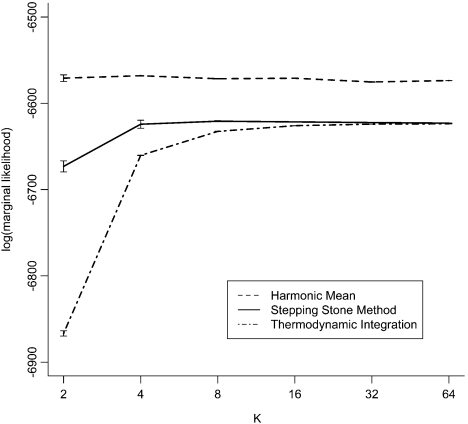
Given that TI and SS are more expensive, computationally, than HM, we were interested in how little computation is necessary for estimating the marginal likelihood accurately. Is K = 50 large enough for this 10-taxon example? Could one get away with using far fewer values of β? To examine this, we conducted a series of MCMC analyses in which only the number of β intervals (K) was changed. For these analyses, the GTR+G model was used with the following priors: Exponential(1.0) for branch lengths, Exponential(1.0) for the shape parameter of the four-category discrete gamma distribution of rates across sites, Dirichlet(1.0,1.0,1.0,1.0,1.0,1.0) for the joint prior on the six GTR relative rates, and Dirichlet(1.0,1.0,1.0,1.0) for joint prior on the four nucleotide frequencies. As before, samples were taken every 10 cycles, and the MCMC analysis explored each β value for 10,000 cycles. As before, the MCMC analyses used for estimating HM were designed to be comparable in sampling effort with those used for estimating TI and SS. For each value of K, 30 independent MCMC analyses were performed for the purpose of estimating the standard error.

The results (Fig. 5) demonstrate that eight β intervals are sufficient for estimating the marginal likelihood using SS for this data set. The aforementioned bias in SS associated with expressing the marginal likelihood on the log scale is also obvious, and clearly a function of the MCMC variance. TI requires a larger number of β intervals than SS in order to overcome its additional discretization bias. Given sufficiently large K, both TI and SS estimate the log marginal likelihood to be − 6617, whereas HM estimates it to be 65 log units higher ( − 6552).

FIGURE 5.

Log marginal likelihood for three estimation methods as a function of the number of β intervals, K, for the green plant Ribulose Bisphosphate Carboxylase/Oxygenase large subunit (rbcL) example. β values are evenly spaced quantiles from a Beta(0.3,1.0) distribution. Error bars represent ±1 standard error based on 30 independent MCMC analyses.

Simulation Study Comparing Models Selected by HM versus SS

One might argue that if HM always chose the same model as TI or SS, then it is irrelevant that HM overestimates marginal likelihoods. That is, even if HM is off the mark, as long as it covaries with the true marginal likelihood, it may nevertheless be an effective way to choose among models. We conducted simulations comparing model selection using HM versus SS to see if 1) they always choose the same model and 2) if they do not choose the same model, which (HM or SS) tends to choose the simpler model. Data sets were simulated by first drawing a number of taxa and a number of sites at random. A discrete uniform distribution was used for each of these choices, with the number of taxa ranging from 4 to 20 (inclusive) and the number of sites from 50 to 5000 (inclusive). For each simulated data set, a tree topology was chosen at random from all possible unrooted, labeled, binary tree topologies (i.e., the proportional-to-distinguishable model), and internal branch lengths, external branch lengths, base frequencies, and GTR relative rates were drawn from Gamma(10, 0.001), Gamma(1.0, 0.1), Dirichlet(100, 100, 100, 100) and Dirichlet(100, 100, 100, 100, 100, 100) distributions, respectively. The discrete gamma distribution (10 categories) was used to impart among-site rate heterogeneity, with the gamma shape parameter drawn from a Gamma(2,3) distribution. The 100 data sets used for this example were thus iid (independently and identically distributed). Although this generating model technically produced all data sets from a GTR+G distribution, the distributions were chosen such that the parameter vectors used for many simulation replicates were arbitrarily close to various submodels of the GTR+G model. For example, the Gamma(2,3) distribution used to choose the shape parameter for among-site rate heterogeneity produces values greater than 5 (i.e., very low rate heterogeneity) about 50% of the time. Thus, about 50% of data sets could be fit nearly as well by the GTR model as by the (true) GTR+G model.

Each of the 100 data sets was subjected to 12 MCMC analyses (6 models for both HM and SS) for a total of 1200 MCMC analyses. The 6 models tested were: Jukes–Cantor (JC) model, JC+G, HKY, HKY+G, GTR, and GTR+G. Priors used were as follows: Exponential(10) for all branch lengths; Dirichlet(1.0,1.0,1.0,1.0) for base frequencies in HKY and GTR models; Dirichlet(1.0,1.0,1.0,1.0,1.0,1.0) for relative rates in GTR models; BetaPrime(1.0,1.0) for the transition/transversion rate ratio parameter (κ) in the HKY model; and Uniform(0,200) for the discrete gamma shape parameter in the “+G” models. The BetaPrime distribution (also known as the “Beta distribution of the second kind”) makes it possible to place a prior on κ in the HKY model that is equivalent to the Dirichlet prior placed on relative rates in the GTR model. That is, the BetaPrime distribution assumed for κ is equivalent to letting κ = p/(1 − p), where p is a Beta(1.0,1.0) random variable. The priors assumed thus correspond exactly to the default priors used in MrBayes v. 3.1.2 (Ronquist and Huelsenbeck 2003). For the SS analyses, 5000 MCMC cycles were devoted to each of the K = 50β intervals, with a preanalysis burn-in of 5000 cycles. To be fair, HM analyses were allowed a 5000 cycle burn-in followed by 50×5000 = 250,000 cycles of sampling. For both HM and SS, samples were taken every 20 cycles during the post-burn-in part of the MCMC analysis. Both simulations and MCMC analyses were performed using Phycas (www.phycas.org).

HM chose the same model as SS in 30 of the 100 simulation replicates (Table 3). In 67 of the remaining 70 simulation replicates (95.7%), SS choose a model that was less complex (in terms of the number of free parameters) than HM. In the 3 cases where HM chose the simpler model, HM chose a rate homogeneity model over a rate heterogeneity model. In contrast, SS often chose models that were much simpler than that chosen by HM: HKY over GTR (25 cases), JC over GTR (21 cases) or JC over HKY (7 cases). HM chose the most complex model possible (GTR+G) in 64% of the simulations. Although the GTR+G is technically the correct model for all simulations, many simulation replicates come very close to much simpler models. For example, in one case in which SS chose JC+G and HM chose GTR+G, the base frequencies and relative rates used for the simulation were π_A = 0.24380, π_C = 0.25456, π_G = 0.24941, π_T = 0.25223 and r_AC = 0.18519, r_AG = 0.16276, r_AT = 0.16649, r_CG = 0.16659, r_CT = 0.18298, r_GT = 0.13598, respectively, which indeed is very close to the π_A = π_C = π_G = π_T = 0.25 and r_AC = r_AG = r_AT = r_CG = r_CT = r_GT = 0.167 characterizing the JC model. This example further illustrates the fact that HM does not impose the correct penalty for unnecessary parameters, which can lead to choosing models that are more complex than those chosen on the basis of accurate marginal likelihoods.

TABLE 3.

Results from simulations pitting HM against SS

HM winner	SS winner
	JCa	JC+Gb	HKYc	HKY+Gd	GTRe	GTR+Gf
JC	0	1	0	0	0	0
JC + G	0	5	0	0	0	0
HKY	0	5	1	1	0	0
HKY + G	1	7	0	8	0	0
GTR	1	2	1	2	0	1
GTR + G	2	21	0	25	0	16

^aJukes–Cantor model.

^bJukes–Cantor model with discrete gamma rate heterogeneity.

^cHasegawa–Kishino–Yano model.

^dHasegawa–Kishino–Yano model with discrete gamma rate heterogeneity.

^eGeneral time reversible model.

^fGeneral time reversible model with discrete gamma rate heterogeneity.

DISCUSSION

In this paper, we introduce the SS method for estimating the marginal likelihood of a model, and compare this with the existing HM method and the TI method. As pointed out by others (e.g., Lartillot and Philippe 2006), the HM method greatly overestimates the marginal likelihood. Furthermore, HM is relatively insensitive to priors: the same estimated marginal likelihood results whether the prior is flat or informative as long as the prior does not prevent the model from reaching areas of highest likelihood. Although insensitivity to priors can, in some contexts, be a good thing, in the BF context, it robs HM of the ability to detect when a model is unnecessarily complex. In phylogenetics, the largest use of HM-derived BFs to date lies in comparing different partitioning strategies. Partitioning simultaneously adds many parameters to a model while at the same time reducing the number of sites available for estimating each parameter. Partitioning is thus an area in which the method used to estimate marginal likelihoods is expected to make a considerable difference (see Fan et al. 2010).

The TI method is far more accurate than HM; however, Lartillot and Philippe (2006) recommended a β increment of 0.01, which requires MCMC samples from 101 β values, making TI considerably more computationally costly than HM. We found that the TI method could be made dramatically more efficient by choosing β values according to evenly spaced quantiles of a Beta(α,1.0) distribution rather than spacing β values evenly from 0.0 to 1.0. This approach generalizes the method suggested by Friel and Pettitt (2008), which corresponds to the special case α = 0.25, and is analogous to the sigmoidal function proposed by Lepage et al. (2007) in a model-switch TI framework. The value α = 0.3 was close to optimal for both our normal distribution example as well as a phylogenetic example (results not shown), suggesting that values close to α = 0.3 are perhaps generally optimal. The choice α = 0.3 results in half of the β values evaluated being less than 0.1. The positive skewness of this distribution is useful because (with sufficient and informative data) the likelihood only begins losing control over the power posterior for β values near 0, and at that point the target distribution changes rapidly from something resembling the posterior to something resembling the prior. Conditioning on the total number of β values evaluated, placing most of the computational effort on β values near zero results in increased accuracy.

The SS method is an importance-sampling approach that uses the power posterior defined by β_{k − 1} as the importance density for estimating the ratio r_k of normalizing constants c_βk/c_{βk − 1}, where k = 1,2,…,K. The overall ratio r is the product of all K ratios. Each ratio r_k thus forms one “stepping stone” along the path bridging posterior and prior distributions. If K = 1, SS is equivalent to the AM method because the prior is used as the importance-sampling density and there is only one “stone” in the path (i.e., the ratio r is estimated directly). The SS method serves as a viable alternative to the annealing-melting form of TI proposed by Lartillot and Philippe (2006). A more general version of SS, described elsewhere (Fan et al. 2010), is more analogous to the model-switch form of TI. In a real example involving protein-coding data from green plants, the log marginal likelihood estimated by SS was less biased than the estimate produced by TI. SS also requires slightly less computational effort than TI due to the fact that, for SS, no samples from the posterior are needed. The bias in SS arises from transformation to the log scale and is directly proportional to the MCMC variance of the estimated log marginal likelihood. This variance is largest for small values of K and can thus be alleviated by using a sufficiently large value of K. One open question is just what constitutes a sufficiently large value of K, and further work is needed to answer the question of how K should scale with the size and complexity of data sets.

We showed through our simulation experiment that HM often provides the same rank order of models as SS. Arguing because of this that HM provides a less costly alternative to SS and TI is specious because HM is supposed to estimate the marginal model likelihood, and it utterly fails at that task. Imagine that we invented a new type of tuning fork that always resonates at a frequency somewhat higher than the fundamental frequency of its nominal note. One could argue that although use of these tuning forks results in very poorly tuned musical instruments, at least the relative order of the notes is preserved! How well would such a product sell, however, given very accurate (but perhaps more expensive) alternatives? Using relative model ranking as an argument for HM is analogous. Our simulations also showed that HM does not always rank models the same way as SS or TI. When they differ, HM tends to choose the more complex model because it fails to adequately penalize the more complex models for having extra parameters that contribute little to model fit. This is direct consequence of the fact that it poorly estimates the marginal likelihood: if it were a good estimator, it would correctly penalize complex models.

The HM method is often criticized for having a large variance (which can be infinite). It often appears to have a very reasonable variance. For example, in Figure 5, the variance of the HM estimate of the log marginal likelihood does not appear to vary wildly across the 6 independent analyses plotted. In the Appendix, we prove that the HM estimator is biased on both the standard and logarithmic scale. A reviewer of this manuscript, Nicolas Lartillot, convinced us that this bias does not, however, account for the majority of the bias actually observed in Figure 5, and also provided us with the following excellent explanation. Apparently, most of the observed bias arises from the large variance of the HM estimator. To see this, consider the fact that the inverse of HM is an unbiased estimator of the inverse of the marginal likelihood. For very simple examples, it is easy to show that even this theoretically unbiased estimator has a large bias in practice because its unbiasedness depends on extreme values that occur extremely rarely. In the world of finite samples, one never sees these extremely rare values, and thus the sample variance is much lower than the true variance, and there is a strong apparent bias when in fact the underlying estimator has no bias in theory. Thus, the apparent stability of HM on the log scale is deceptive, and provides a false sense of security about the quality of the marginal likelihood estimate provided by HM.

We have considered several practical and philosophical issues related to the use of estimated marginal likelihoods to select models for Bayesian phylogenetic analyses (e.g., whether model selection should be sensitive to prior specification); however, this paper is above all else about estimating the numerical quantity known as the marginal likelihood with accuracy. All of our examples demonstrate that the differences in estimation accuracy between the SS and TI methods are minor compared with the difference between either SS or TI and the HM method. Furthermore, our simulations show that SS can sometimes choose different, and simpler, models than HM due to the fact that HM does not penalize complex models as much as it should for unnecessary parameters. We thus recommend routine use of SS or TI instead of the HM method for Bayesian phylogenetic model selection. Both TI and SS have been implemented in the open-source freely available software package Phycas (www.phycas.org).

SUPPLEMENTARY MATERIAL

Supplementary material, including data files, can be found at http://www.sysbio.oxfordjournals.org/.

FUNDING

This work was supported by the National Science Foundation (EF-0331495 to P.O.L, DMS-0723557 to M.-H.C.) and the National Institutes of Health (GM 70335 and CA 74015 to M.-H.C.).

Appendix

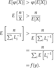
Proof that the expected value of the HM estimator is greater than the true marginal likelihood. Let φ(X) = n/X, where X = ∑_iL_i ^{− 1} and L_i is the likelihood of the ith. sample (i = 1,2,…,n) from the posterior distribution. Note that X > 0 except for the trivial case n = 0. The expected value of each L_i ^{− 1} is

where θ is the vector of model parameters and y represents the data. φ(X) is convex because the second derivative of φ with respect to X is 2n/X³, which is positive because X > 0. By Jensen's inequality,

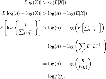
One may argue that the above proof is irrelevant because the HM estimator is always expressed on the log scale. Thus, we prove below that the natural logarithm of the HM estimator is also positively biased.

Proof that the expected value of the log of the HM estimator is greater than the log of the true marginal likelihood. Let φ(X) = log(n) − log(X), where X = ∑_iL_i ^{− 1}. As before, X > 0 and φ(X) is convex because the second derivative of φ with respect to X is 1/X², which is positive. By Jensen's inequality,

References

- Akaike H. A new look at statistical model identification. IEEE Trans. Automat. Contr. 1974;19:716–723. [Google Scholar]
- Alekseyenko AV, Lee CJ, Suchard MA. Wagner and Dollo: a stochastic duet by composing two parsimonious solos. Syst. Biol. 2008;57:772–784. doi: 10.1080/10635150802434394. [DOI] [PMC free article] [PubMed] [Google Scholar]
- Bleidorn C, Eeckhaut I, Podsiadlowski L, Schult N, McHugh D, Halanych KM, Milinkovitch MC, Tiedemann R. Mitochondrial genome and nuclear sequence data support Myzostomida as part of the annelid radiation. Mol. Biol. Evol. 2007;24:1690–1701. doi: 10.1093/molbev/msm086. [DOI] [PubMed] [Google Scholar]
- Brandley M, Schmitz A, Reeder T. Partitioned Bayesian analyses, partition choice, and the phylogenetic relationships of scincid lizards. Syst. Biol. 2005;54:373–390. doi: 10.1080/10635150590946808. [DOI] [PubMed] [Google Scholar]
- Brown JM, Lemmon AR. The importance of data partitioning and the utility of Bayes factors in Bayesian phylogenetics. Syst. Biol. 2007;56:643–655. doi: 10.1080/10635150701546249. [DOI] [PubMed] [Google Scholar]
- Chen M-H, Shao Q.-M. Estimating ratios of normalizing constants for densities with different dimensions. Stat. Sin. 1997;7:607–630. [Google Scholar]
- Chen M-H, Shao Q.-M, Ibrahim JG. Monte Carlo methods in Bayesian computation. New York: Statistics Springer; 2000. [Google Scholar]
- Drummond A, Nicholls G, Rodrigo A, Solomon W. Estimating mutation parameters, population history and genealogy simultaneously from temporally spaced sequence data. Genetics. 2002;161:1307–1320. doi: 10.1093/genetics/161.3.1307. [DOI] [PMC free article] [PubMed] [Google Scholar]
- Fan, Y., Wu R., Chen, M.-H., Kuo L., Lewis P.O. Forthcoming 2010. Choosing among partition models in Bayesian phylogenetics. Mol. Biol. Evol. doi:10.1093/molbev/msq224. [DOI] [PMC free article] [PubMed] [Google Scholar]
- Friel N, Pettitt AN. Marginal likelihood estimation via power posteriors. J. Roy. Statist. Soc. B. 2008;70:589–607. [Google Scholar]
- Gelman A, Meng X-L. Simulating normalizing constants: from importance sampling to bridge sampling to path sampling. Stat. Sci. 1998;13:163–185. [Google Scholar]
- Huelsenbeck JP, Larget B, Alfaro ME. Bayesian phylogenetic model selection using reversible jump Markov chain Monte Carlo. Mol. Biol. Evol. 2004;21:1123–1133. doi: 10.1093/molbev/msh123. [DOI] [PubMed] [Google Scholar]
- Larget B, Simon D. Markov chain Monte Carlo algorithms for the Bayesian analysis of phylogenetic trees. Mol. Biol. Evol. 1999;16:750–759. [Google Scholar]
- Lartillot N, Philippe H. Computing Bayes factors using thermodynamic integration. Syst. Biol. 2006;55:195–207. doi: 10.1080/10635150500433722. [DOI] [PubMed] [Google Scholar]
- Lepage T, Bryant D, Philippe H, Lartillot N. A general comparison of relaxed molecular clock models. Mol. Biol. Evol. 2007;24:2669–2680. doi: 10.1093/molbev/msm193. [DOI] [PubMed] [Google Scholar]
- Li S, Pearl D, Doss H. Phylogenetic tree construction using Markov chain Monte Carlo. J. Am. Stat. Assoc. 2000;95:493–508. [Google Scholar]
- Mau R, Newton MA. Phylogenetic inference for binary data on dendrograms using Markov chain Monte Carlo. J. Comput. Graph. Statist. 1997;6:122–131. [Google Scholar]
- Minin V, Abdo Z, Joyce P, Sullivan J. Performance-based selection of likelihood models for phylogeny estimation. Syst. Biol. 2003;52:674–683. doi: 10.1080/10635150390235494. [DOI] [PubMed] [Google Scholar]
- Newton M, Mau B, Larget B. Markov chain Monte Carlo for the Bayesian analysis of evolutionary trees from aligned molecular sequences. Lect. Notes Monogr. Ser. 1999;33:143–162. [Google Scholar]
- Newton MA, Raftery AE. Approximate Bayesian inference with the weighted likelihood bootstrap (with discussion) J. Roy. Statist. Soc. B. 1994;56:3–48. [Google Scholar]
- Nylander J, Ronquist F, Huelsenbeck J, Nieves-Aldrey J. Bayesian phylogenetic analysis of combined data. Syst. Biol. 2004;53:47–67. doi: 10.1080/10635150490264699. [DOI] [PubMed] [Google Scholar]
- Oehlert GW. A Note on the Delta Method. Am. Stat. 1992;46:27–29. [Google Scholar]
- Pagel M, Meade A. A phylogenetic mixture model for detecting pattern-heterogeneity in gene sequence or character-state data. Syst. Biol. 2004;53:571–81. doi: 10.1080/10635150490468675. [DOI] [PubMed] [Google Scholar]
- Praz CJ, Müller A, Danforth BN, Griswold TL, Widmer A, Dorn S. Phylogeny and biogeography of bees of the tribe Osmiini (Hymenoptera: Megachilidae) Mol. Phylogenet. Evol. 2008;49:185–97. doi: 10.1016/j.ympev.2008.07.005. [DOI] [PubMed] [Google Scholar]
- Rannala B, Yang Z. Probability distribution of molecular evolutionary trees: a new method of phylogenetic inference. J. Mol. Evol. 1996;43:304–311. doi: 10.1007/BF02338839. [DOI] [PubMed] [Google Scholar]
- Ronquist F, Huelsenbeck JP. MRBAYES 3: Bayesian phylogenetic inference under mixed models. Bioinformatics. 2003;19:1572–1574. doi: 10.1093/bioinformatics/btg180. [DOI] [PubMed] [Google Scholar]
- Schwarz GE. Estimating the dimension of a model. Ann. Statist. 1978;6:461–464. [Google Scholar]
- Suchard M, Weiss R, Sinsheimer J. Bayesian selection of continuous-time Markov chain evolutionary models. Mol. Biol. Evol. 2001;18:1001–1013. doi: 10.1093/oxfordjournals.molbev.a003872. [DOI] [PubMed] [Google Scholar]
- Wilks SS. The large-sample distribution of the likelihood ratio for testing composite hypotheses. Ann. Statist. 1938;9:60–62. [Google Scholar]
- Yang Z, Rannala B. Bayesian phylogenetic inference using DNA sequences: a Markov chain Monte Carlo method. Mol. Biol. Evol. 1997;14:717–724. doi: 10.1093/oxfordjournals.molbev.a025811. [DOI] [PubMed] [Google Scholar]
Associated Data
This section collects any data citations, data availability statements, or supplementary materials included in this article.