Macromolecular Docking Restrained by a Small Angle X-Ray Scattering Profile

Abstract

While many structures of single protein components are becoming available, structural characterization of their complexes remains challenging. Methods for modeling assembly structures from individual components frequently suffer from large errors, due to protein flexibility and inaccurate scoring functions. However, when additional information is available, it may be possible to reduce the errors and compute near-native complex structures. One such type of information is a small angle X-ray scattering (SAXS) profile that can be collected in a high-throughput fashion from a small amount of sample in solution. Here, we present an efficient method for protein-protein docking with a SAXS profile (FoXSDock): generation of complex models by rigid global docking with PatchDock, filtering of the models based on the SAXS profile, clustering of the models, and refining the interface by flexible docking with FireDock. FoXSDock is benchmarked on 124 protein complexes with simulated SAXS profiles, as well as on 6 complexes with experimentally determined SAXS profiles. When induced fit is less than 1.5Å interface C_⟨ RMSD and the fraction residues of missing from the component structures is less than 3%, FoXSDock can find a model close to the native structure within the top 10 predictions in 77% of the cases; in comparison, docking alone succeeds in only 34% of the cases. Thus, the integrative approach significantly improves on molecular docking alone. The improvement arises from an increased resolution of rigid docking sampling and more accurate scoring.

Introduction

Many proteins are components of complexes, interacting with other proteins to deliver their functions, such as signal transduction, transport, and catalysis (Krogan et al., 2006; Robinson et al., 2007). Thus, structural description of protein complexes is important for understanding these processes. However, the number of solved complex structures remains relatively low, even while the number of experimentally solved single protein structures increases (Dutta and Berman, 2005). This gap can be bridged by hybrid or integrative methods(Alber et al., 2008; Alber et al., 2007; Steven and Baumeister, 2008). Integrative methods determine complex architectures by computationally combining information from different methods, such as X-ray crystallography or nuclear magnetic resonance (NMR) spectroscopy of component structures, electron microscopy of whole complexes, chemical cross-linking of components detected by mass spectrometry, and small angle X-Ray scattering (SAXS) of complexes.

The computational docking problem, which aims to predict a binary complex starting from the structures of unbound components, has been studied for more than three decades (Katchalski-Katzir et al., 1992; Wodak and Janin, 1978). Docking methods can be classified into three classes based on the sampling algorithms (Ritchie, 2008; Vajda and Kozakov, 2009): global search methods using the fast Fourier transform (FFTs) (Eisenstein and Katchalski-Katzir, 2004) or geometric shape matching (Schneidman-Duhovny et al., 2003), medium-range Monte Carlo methods (Fernandez-Recio et al., 2003; Gray et al., 2003), and the restraint-guided methods (van Dijk et al., 2005). Each class of methods is suitable for a specific docking sub-problem. Global methods are required for an adequate coverage of the search space, medium-range methods are best for local search and refinement, and restraint-guided methods perform well when additional information is available and can be translated into spatial restraints.

Docking methods have been systematically and prospectively evaluated at Critical Assessment of PRedictions of Interactions (CAPRI), relying on target complexes without available structures at the time of prediction (Janin, 2005). It is clear that the state-of-the-art docking methods can successfully (within top 10 predictions) predict the complex structure of two components with limited conformational change upon binding (induced fit that involves rotations of a few side chains), a standard size interface area (change in solvent accessibility area upon complex formation is between 1400 Ų and 2000 Ų), and significant hydrophobic interaction (solvation free energy of complex formation is less than - 4 kcal/mol) (Vajda, 2005). Predictions can also be accurate if additional experimental information about the interaction is available, such as mutations and cross-linking that help identify binding site residues. However, docking methods still suffer from a relatively high rate of incorrect prediction, due to protein flexibility and lack of a reliable scoring function (Lensink et al., 2007; Mendez et al., 2003; Mendez et al., 2005).

SAXS measurement is emerging as a rapid and effective way for obtaining low-resolution (10-30Å) structural information about macromolecular structures in solution (Petoukhov and Svergun, 2007; Putnam et al., 2007). The scattering curve resulting from the subtraction of the buffer from the sample, (SAXS profile, I(q)), is radially symmetric (isotropic) due to the randomly-oriented distribution of particles in solution. The profile can be converted into a radial distribution function of the molecule via a Fourier transform. Unlike electron microscopy, NMR spectroscopy, and X-ray crystallography, SAXS experiments can be performed under a wide variety of solution conditions, including near physiological conditions. The measurement is performed with ~1.0 mg/ml of a macromolecular sample in a ~15 μl volume, and usually takes only a few minutes on a well-equipped synchrotron beam line (Hura et al., 2009; Tsuruta and Irving, 2008).

Computational approaches for modeling a macromolecular structure based on its SAXS profile can be classified into ab initio and rigid body modeling methods (Putnam et al., 2007). On the one hand, the ab initio methods search for coarse shapes represented by dummy atoms (beads) that fit the experimental SAXS profile (Chacon et al., 1998; Svergun, 1999; Svergun et al., 2001). On the other hand, rigid body approaches search for an atomic model of the molecule with a computed SAXS profile that fits the experimental profile (Förster et al., 2008; Pelikan et al., 2009; Petoukhov and Svergun, 2005). Therefore, rigid body modeling can be used only if an approximate structure of the studied molecule or its components are available, as is the case in protein-protein docking.

There are several methods for rigid docking with a SAXS profile. DIMFOM, GLOBSYMM and SASREF (Petoukhov and Svergun, 2005) are based on the CRYSOL program (Svergun et al., 1995) for SAXS profile fitting with a simplified sampling algorithm, where the structure of one monomer is rolled over the surface of the other; however, no interface optimization is performed. In another method, the scoring function combines SAXS and simple interface complementarity terms, sampled by a local search method that requires a relatively accurate initial configuration (Förster et al., 2008); in the absence of the initial configuration, the method starts from 1000 random orientations. A number of analyses of specific biological systems relied on docking followed by filtering of models based on a fit to a SAXS profile (Covaceuszach et al., 2008; Filgueira de Azevedo et al., 2003; Sondermann et al., 2005).

Here, we present a hybrid approach that computes a model of a complex for two given component structures, by simultaneously satisfying physicochemical complementarity between the components as well as a fit to a SAXS profile. The SAXS profile allows to increase the configurational sampling precision and decrease the number of inaccurate models with good scores. Moreover, while docking methods optimize interface shape complementarity, a SAXS profile provides information about the global complex shape. In many cases, especially if the proteins are elongated, small changes in the interface can lead to large changes in the global complex shape. Therefore, it is necessary to increase the sampling resolution to sample the complex accurately in terms of its interface as well as global shape. We test the method on 124 cases with simulated SAXS profiles and six cases with experimental SAXS profiles. The hybrid approach significantly improves on molecular docking alone: When induced fit is less than 1.5Å interface C_⟨ RMSD and the fraction residues missing from the component structures is less than 3%, FoXSDock can find a model close to the native structure within the top 10 predictions in 77% of the cases; in comparison, docking alone succeeds in only 34% of the cases.

Method

Method Outline

The method presented here addresses the docking problem restrained by a SAXS profile: Given two structures of molecules (referred to as a receptor and a ligand) and the SAXS profile of their complex, the goal is to find the complex structure; only minor conformational changes, such as side chain repacking, are explicitly modeled.

The docking protocol involves five steps (Figure 1):

1. Global search. Rigid docking is performed by a geometric shape-matching algorithm PatchDock, generating thousands of models. In this step, the flexibility is taken into account implicitly by allowing a small amount of steric clashes at the interface.

2. Coarse SAXS filtering. Radius of gyration predicted from the SAXS profile of the complex is used to filter out rigid docking models that do not agree with the SAXS measurements.

3. SAXS scoring. Each docking model is fitted against the SAXS profile of the complex.

4. Clustering. Remaining docking models are clustered by their interface C_⟨ RMSD and the cluster representative with the best fit to the SAXS profile is selected.

5. Conformational refinement. Cluster representatives are refined and steric clashes are removed through optimization of side chain positions and relative protein orientations, with FireDock. The final models are scored and ranked by an energy-based score and the fit to the SAXS profile.

Figure 1.

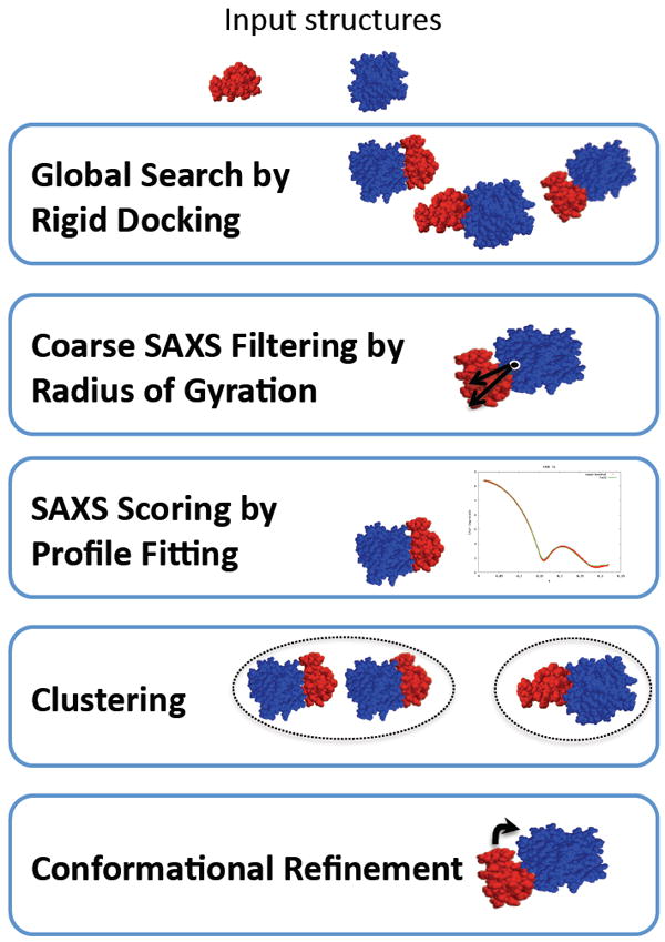
Five stages of FoXSDock are indicated.

Global Search

Rigid Binary Docking

PatchDock is used for global rigid docking (Duhovny et al., 2002; Schneidman-Duhovny et al., 2005b). PatchDock is an efficient rigid docking method that maximizes geometric shape complementarity. To account for surface flexibility in real-life docking involving unbound component structures, the geometric shape complementarity scoring function allows a small amount of steric clashes at the interface. The molecular docking is similar to assembling a jigsaw puzzle. Given two molecules, their surfaces are divided into patches based on their shape: convex, flat, and concave. Once the patches are defined, a pair of neighboring patches on one molecule is superimposed with a pair of neighboring patches on the other molecule, using Geometric Hashing (Lamdan and Wolfson, 1988). Next, the resulting models are clustered, filtered for severe steric clashes, and scored by shape complementarity. The configurational sampling precision can be controlled by the resolution of the surface representation (minimal distance between surface points used to generate docking models) and clustering parameters. Usually, docking methods balance configurational sampling precision against the accuracy and efficiency of scoring function, with the goal of retaining a sufficiently accurate model within a sufficiently small fraction of the best scoring models.

Here, the configurational sampling precision is increased to ensure the complex is sampled accurately in terms of its interface as well as global shape. The final clustering of rigid docking models is performed with a 2Å cut-off on the ligand interface C_⟨ RMSD (compared to the default of 4Å; the ligand interface C_⟨ RMSD is computed using the ligand C_⟨ atoms within 10Å from the receptor in the docked configuration) and the resolution of surface representation of the ligand is decreased by 0.5Å to 1Å. These changes result in the average of 1.7 10⁵ rigid docking models per complex, compared to 8.2 10³ for the default parameter values. In addition, near-native models (ligand C_⟨ RMSD (L-RMSD) < 10Å or interface C_⟨ RMSD (I-RMSD) < 4Å as defined below in the assessment criteria) are observed in 94% of the benchmark cases, compared to 80% for default parameters.

Rigid Multi-Body Symmetric Docking

Symmetric cases are docked with SymmDock (Schneidman-Duhovny et al., 2005a), a docking algorithm for the prediction of cyclically symmetric complexes (C_n) given the structure of its asymmetric unit and symmetry order n. SymmDock a priori restricts its transformational search space only to symmetric transformations, and thus gains both in efficiency and accuracy. In the case of dihedral symmetry (D₂ tetramer is a dimer of dimers), SymmDock is applied first to generate dimers. Next, D₂ tetramers are constructed by combining dimer pairs with perpendicular symmetry axes.

Coarse SAXS Filtering

For a SAXS profile, radius of gyration (R_G^exp) is computed from the slope of the Guinier plot of the profile (Guinier and Fournet, 1955). For a protein structure, radius of gyration (R_G^3D) is computed as $R_G^{3D}=\sqrt{\frac{1}{N}{\displaystyle \sum _{k=1}^N{(r_k-r_c)}^2}}$, where r_k is a position of atom k, and r_c is the centroid of the structure.

A docking model is filtered out if its radius of gyration is 10% smaller or 4% larger than the radius of gyration computed from the SAXS profile (0.9R_G^exp ≤ R_G^3D ≤ 1.04R_G^exp); the larger tolerance for the lower bound results from ignoring the hydration layer in the radius of gyration calculation.

SAXS Profile Fitting

For a given structure or a model, the SAXS profile is computed by FoXS (Schneidman-Duhovny et al.), based on the Debye formula (Debye, 1915):

$$I(q)=\sum _{i=1}^N\sum _{j=1}^N{f}_i(q)f_j(q)\frac{\sin ({\mathit{qd}}_{\mathit{ij}})}{{\mathit{qd}}_{\mathit{ij}}}$$ (1)

where the intensity, I(q), is a function of the momentum transfer, q = (4π sin θ) / λ; 2θ is the scattering angle and λ is the wavelength of the incident X-ray beam; f_i(q) is the form factor of an atom i, d_ij is the distance between atoms i and j, and N is the number of atoms in the system. In the FoXS model, the form factor f_i(q) takes into account the displaced solvent as well as the hydration layer:

$$f_i(q)=f_v(q)-c_1{f}_s(q)+c_2{s}_i{f}_w(q)$$ (2)

where f_v(q) is the atomic form factor in vacuo (Svergun et al., 1995), f_s(q) is the form factor of the dummy atom that represents the displaced solvent (Fraser et al., 1978), s_i is the fraction of the solvent accessible surface of the atom i (Connolly, 1983), and f_w(q) is the water form factor. The parameter c₁ is used to adjust the total excluded volume of the atoms (default value is 1.0) and c₂ is used to adjust the density of the water in the hydration layer (default value is 0.0). In this work, the default values for c₁ and c₂ are used, because we want to rank docking models based on their SAXS fitting scores calculated under identical conditions.

The SAXS profile computed from the structure is fitted to the experimental SAXS profile by minimizing Χ:

$$\chi =\sqrt{\frac{1}{M}{\sum _{i=1}^M\left(\frac{I_{\exp }(q_i)-cI(q_i)}{\sigma (q_i)}\right)}^2}$$ (3)

where I_exp(q) and I(q) are the experimental and computed profiles, respectively, σ(q) is the error of the experimental profile, M is the number of points in the profile, and c is the scaling factor.

For rigid binary docking, additional speed-up is achieved by pre-computing rigid body profiles (I_A, I_B), made possible by constant distances for atom pairs within a rigid body. Only the contribution of inter-rigid body distances to the complex profile (I_AB) is computed for each docking model by iterating over inter-molecular atom pairs in Equation 1. The profile of the docked complex is computed as the sum of three profiles: I_complex = I_A+ I_B+I_AB.

For symmetric complexes, even higher speed-up can be achieved, because the symmetric complex contains multiple copies of the symmetry unit. For dihedral symmetry D₂, the profile is given by I_complex = 4I_A+ 2I_AB+2I_AC+2I_AD (Figure 2a). For cyclic symmetry C_n, all distances between the symmetry units can be computed based on the distances between the first unit and n/2 other units in the complex. The complex profile is computed as $I_{\mathit{complex}}={\mathit{nI}}_{u_0}+n{\displaystyle \sum _{i=1}^{n/2-1}{I}_{u_0{u}_i}+cn{I}_{u_0{u}_{n/2}}}$, where U_i is unit i in the symmetric complex, c=1 if n is odd, and c=0.5 if n is even (Figure 2b).

Figure 2.

SAXS profile computation for symmetric assemblies. Only the distances between the units marked with arrows are computed. (a) Tetramer with dihedral symmetry D₂. (b) Symmetric assembly with cyclic symmetry C_n.

Clustering

The models are clustered iteratively, as follows. The clustering starts with the docking model that has the lowest Χ score. This model becomes a representative of the current cluster and the C_⟨ atoms in the binding site of its ligand (ie, the ligand C_⟨ atoms within 10Å from the receptor in the docked configuration) provide the frame of reference for calculating the ligand interface C_⟨ RMSD for each one of the remaining (unclustered) models. All models with a ligand interface C_⟨ RMSD below 4Å are assigned to the current cluster. When the cluster can no longer be expanded, the docking model with the lowest Χ score from the unclustered set of models initiates a new cluster.

Conformational Refinement

The steric clashes, introduced by PatchDock, are removed with FireDock (Andrusier et al., 2007; Mashiach et al., 2008) that refines side chain positions and relative protein orientations. After steric clashes are removed, an energy-like function is used to rank the docking models. This interface energy score is a weighted combination of softened van der Waals, desolvation, electrostatics, hydrogen bonding, disulfide bonding, π-stacking, aliphatic interactions, and rotamer preferences (Andrusier et al., 2007).

Composite Score and Ranking

The interface energy score and SAXS profile fitting scores (∣ values) of the final docking models are rescaled independently to the [0-1] interval and the composite score is computed as: S_Composite = S_Energy + 0.3S_SAXS, where S_Energy and S_SAXS are the rescaled scores and 0.3 is the weight of the SAXS term. This weight was determined by enumerating a range of weight values to maximize the number of cases with near-native model within 10 top scoring models. Half of the Benchmark 1 randomly selected cases were used to determine the weight and the other half was used for validation.

Benchmark

We test the method with two types of data. First, each test case consists of unbound component structures and a simulated SAXS profile for their complex. Second, each test case consists of bound component structures and an experimentally obtained SAXS profile for their complex.

Benchmark 1 - Simulated SAXS profiles

Protein-protein docking benchmark 3.0 (Hwang et al., 2008) is used for method validation with computed SAXS profiles. This benchmark contains 124 unbound-unbound test cases, classified into 88 rigid-body cases (I-RMSD ≤ 1.5Å), 19 medium-difficulty cases (1.5Å < I-RMSD ≤ 2.2Å), and 17 difficult cases (I-RMSD > 2.2Å). The complexes are also classified into three biochemical categories: enzyme–inhibitor (35 cases), antigen–antibody (25 cases), and others (64 cases). A SAXS profile is simulated using the co-crystallized structure of the complex for a q range from 0 to 0.5Å^-1. For Χ calculations involving only computed profiles, the relative error is calculated from the Poisson distribution with λ of 10 and bound to 5%.

Benchmark 2 – Experimental SAXS profiles

Experimental SAXS profiles and associated relative errors for 6 complexes (Table 1, Figure 3 - left column) from the BIOSIS database are used (Hura et al., 2009). These cases include three symmetric dimers with cyclic symmetry, two tetramers with dihedral symmetry, and one decamer with dihedral symmetry. The dimers are docked with SymmDock starting from the monomer structure. The tetramers are also docked with SymmDock by exhaustive enumeration of C₂ symmetric models (Methods). For the decamer, we start with the dimer structure and apply SymmDock to build a pentamer of dimers. BIOISIS entries include structures with modeled missing residues. These residues are used for SAXS calculations, but not in docking.

Table 1.

Benchmark 2 cases: PDB codes, complex type, number of residues, fraction of missing residues, R_G^3D (radius of gyration of the complex structure), R_G^exp (radius of gyration computed from the experimental SAXS profile), Χ value for the fit between the experimental and computed SAXS profiles with and without fitting parameters. Disordered regions were added in BIOISIS structure (Hura et al., 2009) in cases marked with *.

PDB	Complex type	Residue number	Fraction of missing residues	RG3D	RGexp	Χ
1YEM*	C2 dimer	356	0	25.70	27.40	3.89 (7.81)
3F7L	C2 dimer	302	0	20.02	20.66	3.23 (13.28)
2DVM*	C2 dimer	948	0	32.98	32.83	2.88 (2.95)
2E2G	D5 decamer	2382	1.6	50.97	51.24	7.72 (8.37)
2G4J	D2 tetramer	1544	0	31.77	31.08	4.69 (14. 93)
1DQK	D2 tetramer	496	0	21.07	22.39	4.78 (21.35)

Figure 3.

Benchmark 2 complexes and SAXS profile fitting scores. In the first column, experimental SAXS profiles (red) and the computed profiles (green) from complex structures (ribbons) for Benchmark 2 cases are shown. The plots in the second column display SAXS scores (Χ values on the y-axis) as a function of C_⟨ RMSD (x-axis) for all models from the rigid docking stage. The third column plots the SAXS profile fitting score versus R_G^3D for the same set of complexes. The color-coding reflects the C_⟨ RMSD. The black line indicates the R_G^exp and the grey lines show the thresholds for filtering.

Assessment Criteria

An assessment criterion similar to that from CAPRI is used (Lensink et al., 2007). A docking model is considered acceptable (one star) if a ligand C_⟨ RMSD (L-RMSD) after superposition of the receptor is below 10Å or interface C_⟨ RMSD (I-RMSD) is below 4Å. A docking model is of medium accuracy (two stars) if L-RMSD < 5Å or I-RMSD < 2Å, and of high accuracy (three stars) if L-RMSD < 1Å or I-RMSD < 1Å. A docking model of acceptable or better accuracy is referred to as near-native. For symmetric complexes, C_⟨ RMSD is computed after least-squares-fit superposition of the model on the native complex. Symmetric docking model is considered near-native if C_⟨ RMSD is below 5Å.

Results

We begin by assessing the accuracy of the radius of gyration computed from a SAXS profile, followed by quantifying the match between an experimental SAXS profile and a SAXS profile computed for the native complex. Finally, we assess FoXSDock by its performance on the two benchmarks.

Accuracy of predicted radius of gyration

We first assess to what degree the radius of gyration (R_G^exp) computed from the SAXS profile of the complex fits the radius of gyration (R_G^3D) of the complex structure. This analysis is used to find the threshold values for coarse SAXS filtering stage. In Benchmark 1 with simulated SAXS profiles, we compared the R_G^exp to the R_G^3D of the best possible docking models (Table S1). The best possible docking model is constructed by superposing unbound components to the complex structure. In Benchmark 2 with experimental SAXS profiles, the R_G^exp is compared with the R_G^3D of the complex structures (Table 1). In Benchmark 1, the R_G^exp is predicted with 2.18% accuracy (average) for cases with less than 3% missing residues (81 cases out of 124). The fractional difference in the number of residues in the complexes with bound and unbound structures is referred to as the fraction of missing residues. We conclude that R_G measure is not very sensitive to conformational changes upon binding. Thus, it is possible to compute an accurate R_G^3D even when using unbound components for docking. In Benchmark 2, the R_G^exp can be up to ~7% larger than the R_G^3D. One possible explanation is that the hydration layer of a protein is not taken into account when computing R_G^3D from the coordinates of protein atoms.

Based on the numbers above, the thresholds for coarse SAXS filtering by R_G^exp are set to 0.9R_G^exp and 1.04R_G^exp (ie. a docking model is filtered out if its R_G^3D is more than 10% smaller or 4% larger than the R_G^exp). The R_G^3D of 119 (out of 124) complexes of Benchmark 1 and all the complexes of Benchmark 2 is within these thresholds (0.9R_G^exp ≤R_G^3D≤ 1.04R_G^exp). In the remaining 5 cases of Benchmark 1, the fraction of missing residues is more than 5% or large conformational changes are involved (I-RMSD > 8Å).

Accuracy of profile fit

For Benchmark 1, the profile computed from the complex structure is compared to the profile computed from the best possible docking model of unbound components (Table S1). The best possible docking model is constructed by superposing unbound components to the complex structure. The accuracy of the profile fit is assessed as a function of the fraction of missing residues and the I-RMSD between the bound and unbound component structures (Figure 4). As expected, Χ increases with the increase in the fraction of missing residues and I-RMSD.

Figure 4.

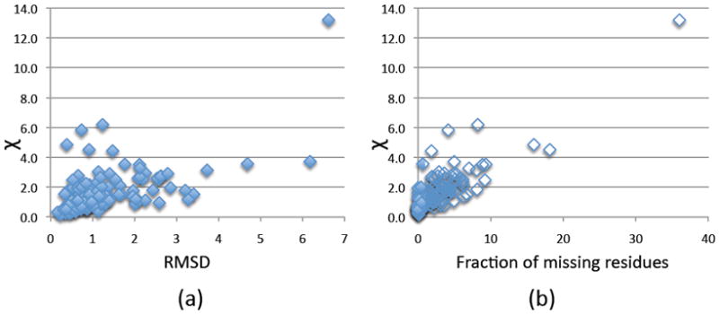
Impact on the SAXS profile fitting by induced fit and missing residues. (a) I-RMSD between complex structures consisting of bound and unbound components as a function of Χ. (b) fraction of missing residues as a function of Χ.

For Benchmark 2, experimental SAXS profiles are compared with profiles computed from the complex structures. In all cases, except 1YEM and 2E2G, a good fit is observed (ie, the experimental and computed profiles overlap for q < 0.2 Å^-1; Figure 3a). The difference between the experimental and computed profiles for 1YEM might be explained by the modeling error for the residues missing in the crystallographic structure as well as by the difference between the solution and crystal structures. For 2E2G, an additional possible cause for the profile mismatch includes the differences between the experimental profile measured for PF1033 from P. furiosus and the profile computed from the homologous structure 2E2G (57% sequence identity).

Accuracy of FoXSDock based on Benchmark 1

Next, we assess each stage of the method to gain a better appreciation of the contribution of each stage to the final accuracy. The goal of each stage is to output as many good scoring near-native models as possible, while eliminating as many non-native models as possible. However, the emphasis on these two aspects changes with the progress through the flowchart. In the initial stages, the priority is to produce as many near-native models as possible, while in the later stages the priority is to rank them highly.

Global Search

The average frequency of near-native models among the output models is 0.0026%, varying from 0 to 1755 models, with the average of 331 near-native models per case (Table S2). The average is higher in the rigid-body cases (413 models) than in the medium and difficult cases (217 and 30 models, respectively). Near-native models are found for all benchmark cases, except for one medium difficulty case and six difficult cases (ie, 117 out of 124 benchmark cases have a model of acceptable or better accuracy after rigid docking with PatchDock). Moreover, 96 cases include at least one model of medium accuracy and 58 cases include a model of high accuracy.

Coarse SAXS Filtering

About one third of all models are eliminated in this stage. Nevertheless, in most cases, near-native models are not filtered out and the average hit rate increases to 0.0037% (Table S2). The average number of near-native models does not change relative to the global search stage (316 versus 331). All near-native models are filtered out only in three cases (1I4D, 1I2M, 1R8S), due to a large error in the computed R_G^exp resulting from a high number of missing residues (Table S1). In practice, missing residues can be accounted by decreasing R_G^exp thresholds and the weight of SAXS component in the composite score.

SAXS Scoring

Ideally, the profile fitting score (Χ) score should be correlated with the accuracy of the model below some usefully large radius of convergence (ie, I-RMSD of ~5Å or L-RMSD of ~10Å). We examine whether or not such a “funnel” exists for each case in Benchmark 1 (Figure 5, first column; Figure S1). Some cases show a clear funnel, such as the first two cases in Figure 5 (1BVN and 1DFJ) with low Χ value models corresponding to near-native structures. Others have additional model clusters with low Χ values (Figure 5, 1CGI and 1TMQ), resulting from widely different configurations with similar overall shapes. For example, if the ligand has a globular shape, all the complexes with the correct ligand-binding site on the receptor have a low Χ, irrespective of the ligand orientation (Figure 5, 1CGI and 1E6E). If the receptor is symmetric, there are a number of ligand clusters with a low Χ value (eg, three clusters for the triangular receptor shape; Figure 5, 2O8V). There are also cases with no funnel at all (Figure 5, 1E6E and 2O8V). However, even in these cases, the scores of near-native complexes are significantly lower than average, so the profile still provides valuable information that eliminates a large number of non-native complexes.

Figure 5.

Use of SAXS information in FoXSDock. Selected Benchmark 1 cases include 1BVN, 1DFJ, 1CGI, 1TMQ, 1E6E, 2O8V in rows one to six, respectively. The plots in the first column display SAXS scores (Χ values on the y-axis) as a function of I-RMSD (x-axis) for all models from the rigid docking stage. The second column plots the SAXS profile fitting score versus R_G^3D for the same set of complexes. The color-coding reflects the I-RMSD. The black line indicates the R_G^exp and the grey lines show the thresholds for filtering. The third column shows models with the lowest Χ scores. The native complex is shown in red in all panels. In the first two cases (1BVN and 1DFJ), the near-native model has the lowest Χ score. For 1CGI and 1E6E, the 10 models with the lowest Χ score do not include any near-native models; however, the binding site of the receptor is accurately identified. For 1TMQ and 2O8V, the 10 models with the lowest Χ score define two and three clusters, respectively, due to the symmetry in the receptor.

We also examine the accuracy of coarse filtering by R_G^exp compared to that by Χ. Plots of the Χ score versus R_G^3D colored by the corresponding accuracy of the model show that both SAXS-based criteria eliminate many non-native models, while retaining the near-native ones (Figures 5 and S1).

Clustering

Clustering eliminates more than 80% of models; the average number of models after clustering is 19,860. The filtered models are ranked according to the Χ value. Overall, there is a top scoring model of acceptable or better accuracy in 24 (19%) cases of the benchmark (Tables 2, S3). Considering the top 10 ranked models, 54 (44%) cases correspond to an acceptable or better model. In 79 (64%) cases, there is a near-native model among the top 100 predictions. In the remaining cases, the rank is in the range from 100 to 5000 (35 cases); near-native model is not found at all in only 10 cases (in 7 cases it is not produced by docking, and in 3 cases it is eliminated by the R_G^exp filtering). Out of the 124 cases in the benchmark, 21 and 63 include high and medium accuracy models.

Table 2.

Summary of Benchmark 1 results. The rows list the number and fraction (in brackets) of benchmark cases with a near-native model within top 1, 10, 100, all 5000 output models, high and medium accuracy models, and the total number of benchmark cases. The columns list the success rate for ranking with (a) SAXS scores only, (b) the composite score that combines the energy-based and SAXS scores, (c-e) the composite score for the enzyme-inhibitor, antibody-antigen, and other complexes separately, (f) the composite score for rigid-body cases, (g) the composite score for rigid-body cases with less than 3% missing residues, and (h) the standard docking protocol without SAXS profile.

	SAXS score onlya	Composite Scoreb	Composite Score EIc	Composite Score AAd	Composite Score Otherse	Composite Score Rigid-bodyf	Rigid-body and <3% missing residuesg	Standard docking protocolh
Top	24 (19%)	32 (26%)	14 (40%)	8 (32%)	10 (16%)	29 (33%)	25 (38%)	12 (10%)
Top 10	54 (44%)	67 (54%)	26 (74%)	17 (68%)	24 (38%)	58 (66%)	50 (77%)	33 (27%)
Top 100	79 (64%)	88 (71%)	30 (86%)	22 (88%)	36 (56%)	75 (85%)	59 (90%)	60 (48%)
All 5000	114 (92%)	110 (89%)	35 (100%)	23 (92%)	52 (81%)	86 (98%)	65 (100%)	99 (80%)
High accuracy	21 (17%)	27 (22%)	9 (26%)	9 (36%)	9 (14%)	25 (28%)	21 (32%)	14 (11%)
Medium accuracy	84 (68%)	84 (68%)	27 (77%)	22 (88%)	35 (55%)	74 (84%)	56 (86%)	58 (47%)
Total	124	124	35	25	64	88	65	124

Conformational Refinement and Final Ranking

We refine 5000 models with the lowest Χ scores after clustering. The models are re-ranked according to the composite score, corresponding to the sum of the energy-based score and Χ. Energy-based scoring brings new information into the protocol, improving model ranking compared to the previous stage. There is a top-scoring model of acceptable or better accuracy in 32 (26%) cases of the benchmark. 67 (54%) cases include an acceptable or better model among the top 10 predictions (Table 2). In 88 cases, there is a near-native model among the top 100 predictions; in 22 cases, the rank is worse or no near-native model is found (14 cases). The accuracy of the models is also improving; there are 27 cases with high accuracy models after refinement.

Success by complex categories

Next, we examine the success of the protocol in different complex categories.

Complex Type

The best performance is obtained for enzyme-inhibitor complexes (26 out of 35 cases have a near-native model among the 10 best scoring models), followed by antibody-antigen complexes (17 cases out of 25 cases have a near-native model among the 10 best scoring models). For other protein-protein complexes, the success rate is lower (only 24 out of 64 cases include near-native models among the 10 best scoring models). Many of these cases have high numbers of missing residues (more than 3% of residues are missing in 33 cases). In such cases, additional improvement might be possible to achieve by accurate modeling of the missing residues.

Induced fit

If we consider only 88 rigid-body cases of the benchmark, the success rate is higher than the overall average. There is a near-native model among the 10 best scoring models in 66% of the cases. Difficult cases require explicit modeling of the backbone flexibility that was not performed in this work. However, the protocol presented here can in principle process docking models from flexible docking as well.

Fraction of Missing Residues

65 of the 88 rigid-body cases have less than 3% missing residues. For this subset, our success rate is the highest, with a near-native model among the 10 best scoring models in 77% of the cases.

Comparison to standard docking protocol

We compare FoXSDock to the standard docking protocol by PatchDock (Duhovny et al.) and FireDock without SAXS profiles (Andrusier et al., 2007). In standard docking, rigid docking models are created with PatchDock and 5000 top scoring models are refined and re-ranked by FireDock. The only difference between the two protocols is that FoXSDock uses a higher configurational sampling precision resulting into an increase from 8.2 10³ to 1.6 10⁵ sampled models per complex (it would be computationally too expensive to refine all of these models by FireDock). The success rate of FoXSDock is much higher than that of standard docking (Table 2). The top-scoring model is near-native in only 12 cases for standard docking, compared to 32 cases for FoXSDock. The number of near-native models among the top 10 models doubles from 33 to 67. The accuracy is also improved; there are 27 cases with high accuracy models compared to 14 without using a SAXS profile.

Accuracy of FoXSDock based on Benchmark 2

The performance of FoXSDock on Benchmark 2 is qualitatively similar to that for Benchmark 1 (Table 3). As expected, rigid docking finds a near-native model in all cases (Columns 2-4 in Table 3); the hit rates are higher compared to Benchmark 1 cases, because the search space is restricted to symmetric complexes only. As before, coarse SAXS filtering by R_G^exp significantly enriches for near-native models (Columns 5-7 in Table 3). There is a strong funnel in the plot of Χ versus C_⟨ RMSD for three cases (Figure 4; 2DVM, 2G4J, 1DQK). Coarse SAXS filtering keeps most of the near-native models (indicated by grey horizontal lines in Figure 4). After Χ scoring for cases with funnels, a near-native model scores best for 2 cases (2DVM, 2G4J), 2^nd best for 1 case (1DQK), while no near-native models are ranked highly for the remaining 3 cases. The rank improves significantly after refinement by FireDock. 5 out of 6 cases have a near-native model among the top 10 models, three of them at the very top. In one case (2E2G, already discussed above) involving a structure of a homolog for which the experimental profile was measured, FoXSDock fails to rank a near-native model among the top 10. It is possible that this case requires additional rigid docking sampling or accurate comparative modeling, because there are only six near-native models among the initial SymmDock-produced models.

Table 3.

Benchmark 2 docking results. Number of near-native models (C_⟨ RMSD after superposition < 5.0 Å) for rigid symmetric docking (columns 2-4) and after coarse SAXS filtering (columns 5-7). Rank and C_⟨ RMSD of the first near-native model after ranking by the SAXS profile fitting score (column 8) and by the composite score (column 9).

PDB	Global Search			Coarse SAXS filtering			SAXS score	Composite score
	Hits	Total	Rate	Hits	Total	Rate	Rank (C⟨ RMSD)	Rank (C⟨ RMSD)
1YEM*	34	3730	0.0091	32	1513	0.0212	32 (3.37)	1 (2.30)
3F7L	37	3044	0.0121	30	1443	0.0207	21 (2.98)	7 (4.08)
2DVM*	6	3727	0.0016	6	1159	0.0052	1 (1.10)	1 (1.53)
2E2G	10	16608	0.0006	6	7829	0.0008	1700 (4.67)	688 (1.08)
2G4J	274	116737	0.0023	155	301	0.0515	1 (3.76)	1 (2.69)
1DQK	174	12012	0.0144	168	2271	0.0739	2 (4.45)	8 (4.55)

Discussion

Overview

Three key points emerge from this study. First, incorporation of a SAXS profile into rigid docking requires increasing configurational sampling precision of docking. Second, a SAXS profile helps to achieve a significant improvement over a standard docking protocol. Third, while helpful, a SAXS profile still provides only limited information about the complex shape; thus, the accuracy of the scoring function for selecting near-native models is a major remaining problem. We discuss each of these points in turn.

Increasing Configurational Sampling Precision

External information, such as a SAXS profile, binding site residues, symmetry, and distance restraints, are ideally incorporated directly into the configurational and/or conformational search algorithm (Andre et al., 2007; Schneidman-Duhovny et al., 2005a; van Dijk et al., 2005). While a SAXS profile provides information about the atomic distance distribution within the complex, generating all docking models with a specified tolerance around a given distance distribution is a challenging problem. Therefore, we take an alternative approach in this work. The configurational sampling precision of rigid docking is increased, followed by filtering out the models that are not consistent with the SAXS profile. The five search and rank stages of FoXSDock are designed to benefit from the increasingly focused molecular docking search space afforded by the knowledge of the SAXS profile. In contrast, most other molecular docking protocols include external information in a single filtering step following the global search.

Improvement Compared to Standard Docking

The method is tested on a large benchmark with computed profiles and six cases with experimental SAXS profiles. Including a SAXS profile helps to achieve a significant improvement over a standard docking protocol: The number of cases with a near-native model at the top almost triples (from 10% to 26%) and doubles if we accept a near-native model within the top 10 scoring models (from 27% to 54%). In rigid-body cases with less than 3% missing residues, FoXSDock can find a model close to the native structure within the top 10 predictions in 77% of the cases, compared to 34% for docking alone. Increasing the configurational sampling precision also helps to improve model accuracy: There are twice as many cases with high accuracy models (27 compared to 14 without using a SAXS profile).

Ranking of Models Remains a Problem

There are three major reasons for failure to produce a near-native model within the top 10 scoring models. First, large conformational changes upon binding do not allow finding a near-native model in the global search (6%). Second, a SAXS profile is sensitive to missing residues. The fraction of distances missing from a SAXS profile is almost double the fraction of the missing part. Third, the scoring function cannot rank a near-native model high (ie, the rank of a near-native model is between 10 and 5000 (35% of the cases – Table 2)).

In summary, we present a method that efficiently combines molecular docking and fitting to a SAXS profile. We expect to find FoXSDock useful in a variety of applications, such as docking with comparative models that is becoming increasingly common at CAPRI (Janin, 2007), flexible docking (Schneidman-Duhovny et al., 2007), and determining structures of multi-component macromolecular assemblies (Inbar et al., 2005; Karaca et al., 2010; Lasker et al., 2009). FoXSDock can also be applied when a SAXS profile is measured for a mixture of the complex and unbound components. In this case, coarse filtering by R_G^exp is not possible and the SAXS scoring stage has to fit a weighted sum of computed profiles of unbound components and a docking model to the experimental profile (Konarev et al., 2003).

Because the accuracy of the scoring function is still a major bottleneck, FoXSDock can be improved further by integrating more external information in addition to the SAXS profile. This information includes binding site residues determined by mutation, conservation analysis, NMR spectroscopy and other approaches; distance restraints determined from cross-linking, hydrogen-deuterium exchange, NMR spectroscopy or FRET spectroscopy; and a density map from electron microscopy. In this way, FoXSDock will contribute to maximizing the accuracy, precision, coverage, and efficiency of the structural characterization of macromolecular assemblies.

Software availability

Source code and executables for SAXS profile calculation and fitting are available as part of the IMP software package (http://salilab.org/imp). A standalone version of FoXS is also available for download and as a web-server from http://salilab.org/foxs. The two benchmarks and the protocol scripts will be available at http://salilab.org/foxs. PatchDock and FireDock are available from http://bioinfo3d.cs.tau.ac.il.

References

- Alber F, Forster F, Korkin D, Topf M, Sali A. Integrating diverse data for structure determination of macromolecular assemblies. Annu Rev Biochem. 2008;77:443–77. doi: 10.1146/annurev.biochem.77.060407.135530. [DOI] [PubMed] [Google Scholar]
- Alber F, Dokudovskaya S, Veenhoff LM, Zhang W, Kipper J, Devos D, Suprapto A, Karni-Schmidt O, Williams R, Chait BT, Rout MP, Sali A. Determining the architectures of macromolecular assemblies. Nature. 2007;450:683–94. doi: 10.1038/nature06404. [DOI] [PubMed] [Google Scholar]
- Andre I, Bradley P, Wang C, Baker D. Prediction of the structure of symmetrical protein assemblies. Proc Natl Acad Sci U S A. 2007;104:17656–61. doi: 10.1073/pnas.0702626104. [DOI] [PMC free article] [PubMed] [Google Scholar]
- Andrusier N, Nussinov R, Wolfson HJ. FireDock: fast interaction refinement in molecular docking. Proteins. 2007;69:139–59. doi: 10.1002/prot.21495. [DOI] [PubMed] [Google Scholar]
- Chacon P, Moran F, Diaz JF, Pantos E, Andreu JM. Low-resolution structures of proteins in solution retrieved from X-ray scattering with a genetic algorithm. Biophys J. 1998;74:2760–75. doi: 10.1016/S0006-3495(98)77984-6. [DOI] [PMC free article] [PubMed] [Google Scholar]
- Connolly ML. Solvent-accessible surfaces of proteins and nucleic acids. Science. 1983;221:709–13. doi: 10.1126/science.6879170. [DOI] [PubMed] [Google Scholar]
- Covaceuszach S, Cassetta A, Konarev PV, Gonfloni S, Rudolph R, Svergun DI, Lamba D, Cattaneo A. Dissecting NGF interactions with TrkA and p75 receptors by structural and functional studies of an anti-NGF neutralizing antibody. J Mol Biol. 2008;381:881–96. doi: 10.1016/j.jmb.2008.06.008. [DOI] [PubMed] [Google Scholar]
- Debye P. Zerstreuung von Röntgenstrahlen. Annalen der Physik. 1915;351:809–823. [Google Scholar]
- Duhovny D, Nussinov R, Wolfson HJ. Efficient Unbound Docking of Rigid Molecules. In: Guigó R, Gusfield D, editors. Second International Workshop, WABI 2002. 2452/2002. Springer; Berlin/Heidelberg, Rome, Italy: 2002. pp. 185–200.pp. 185–200. [Google Scholar]
- Dutta S, Berman HM. Large macromolecular complexes in the Protein Data Bank: a status report. Structure. 2005;13:381–8. doi: 10.1016/j.str.2005.01.008. [DOI] [PubMed] [Google Scholar]
- Eisenstein M, Katchalski-Katzir E. On proteins, grids, correlations, and docking. C R Biol. 2004;327:409–20. doi: 10.1016/j.crvi.2004.03.006. [DOI] [PubMed] [Google Scholar]
- Fernandez-Recio J, Totrov M, Abagyan R. ICM-DISCO docking by global energy optimization with fully flexible side-chains. Proteins. 2003;52:113–7. doi: 10.1002/prot.10383. [DOI] [PubMed] [Google Scholar]
- Filgueira de Azevedo W, Jr, dos Santos GC, dos Santos DM, Olivieri JR, Canduri F, Silva RG, Basso LA, Renard G, da Fonseca IO, Mendes MA, Palma MS, Santos DS. Docking and small angle X-ray scattering studies of purine nucleoside phosphorylase. Biochem Biophys Res Commun. 2003;309:923–8. [PubMed] [Google Scholar]
- Förster F, Webb B, Krukenberg KA, Tsuruta H, Agard DA, Sali A. Integration of small-angle X-ray scattering data into structural modeling of proteins and their assemblies. J Mol Biol. 2008;382:1089–106. doi: 10.1016/j.jmb.2008.07.074. [DOI] [PMC free article] [PubMed] [Google Scholar]
- Fraser RDB, MacRae TP, Suzuki E. An improved method for calculating the contribution of solvent to the X-ray diffraction pattern of biological molecules. Journal of Applied Crystallography. 1978;11:693–694. [Google Scholar]
- Gray JJ, Moughon S, Wang C, Schueler-Furman O, Kuhlman B, Rohl CA, Baker D. Protein-protein docking with simultaneous optimization of rigid-body displacement and side-chain conformations. J Mol Biol. 2003;331:281–99. doi: 10.1016/s0022-2836(03)00670-3. [DOI] [PubMed] [Google Scholar]
- Guinier A, Fournet G. Small-angle scattering of X-rays. John Wiley & sons; 1955. [Google Scholar]
- Hura GL, Menon AL, Hammel M, Rambo RP, Poole FL, 2nd, Tsutakawa SE, Jenney FE, Jr, Classen S, Frankel KA, Hopkins RC, Yang SJ, Scott JW, Dillard BD, Adams MW, Tainer JA. Robust, high-throughput solution structural analyses by small angle X-ray scattering (SAXS) Nat Methods. 2009;6:606–12. doi: 10.1038/nmeth.1353. [DOI] [PMC free article] [PubMed] [Google Scholar]
- Hwang H, Pierce B, Mintseris J, Janin J, Weng Z. Protein-protein docking benchmark version 3.0. Proteins. 2008;73:705–9. doi: 10.1002/prot.22106. [DOI] [PMC free article] [PubMed] [Google Scholar]
- Inbar Y, Benyamini H, Nussinov R, Wolfson HJ. Prediction of multimolecular assemblies by multiple docking. J Mol Biol. 2005;349:435–47. doi: 10.1016/j.jmb.2005.03.039. [DOI] [PubMed] [Google Scholar]
- Janin J. Assessing predictions of protein-protein interaction: the CAPRI experiment. Protein Sci. 2005;14:278–83. doi: 10.1110/ps.041081905. [DOI] [PMC free article] [PubMed] [Google Scholar]
- Janin J. The targets of CAPRI rounds 6-12. Proteins. 2007;69:699–703. doi: 10.1002/prot.21689. [DOI] [PubMed] [Google Scholar]
- Karaca E, Melquiond AS, de Vries SJ, Kastritis PL, Bonvin AM. Building macromolecular assemblies by information-driven docking: introducing the HADDOCK multi-body docking server. Mol Cell Proteomics. 2010 doi: 10.1074/mcp.M000051-MCP201. [DOI] [PMC free article] [PubMed] [Google Scholar]
- Katchalski-Katzir E, Shariv I, Eisenstein M, Friesem AA, Aflalo C, Vakser IA. Molecular surface recognition: determination of geometric fit between proteins and their ligands by correlation techniques. Proc Natl Acad Sci U S A. 1992;89:2195–9. doi: 10.1073/pnas.89.6.2195. [DOI] [PMC free article] [PubMed] [Google Scholar]
- Konarev PV, Volkov VV, Sokolova AV, Koch MHJ, Svergun DI. PRIMUS: a Windows PC-based system for small-angle scattering data analysis. Journal of Applied Crystallography. 2003;36:1277–1282. [Google Scholar]
- Krogan NJ, Cagney G, Yu H, Zhong G, Guo X, Ignatchenko A, Li J, Pu S, Datta N, Tikuisis AP, Punna T, Peregrin-Alvarez JM, Shales M, Zhang X, Davey M, Robinson MD, Paccanaro A, Bray JE, Sheung A, Beattie B, Richards DP, Canadien V, Lalev A, Mena F, Wong P, Starostine A, Canete MM, Vlasblom J, Wu S, Orsi C, Collins SR, Chandran S, Haw R, Rilstone JJ, Gandi K, Thompson NJ, Musso G, St Onge P, Ghanny S, Lam MH, Butland G, Altaf-Ul AM, Kanaya S, Shilatifard A, O’Shea E, Weissman JS, Ingles CJ, Hughes TR, Parkinson J, Gerstein M, Wodak SJ, Emili A, Greenblatt JF. Global landscape of protein complexes in the yeast Saccharomyces cerevisiae. Nature. 2006;440:637–43. doi: 10.1038/nature04670. [DOI] [PubMed] [Google Scholar]
- Lamdan Y, Wolfson HJ. Geometric Hashing: A General And Efficient Model-based Recognition Scheme. Computer Vision., Second International Conference on. 1988:238–249. [Google Scholar]
- Lasker K, Topf M, Sali A, Wolfson HJ. Inferential optimization for simultaneous fitting of multiple components into a CryoEM map of their assembly. J Mol Biol. 2009;388:180–94. doi: 10.1016/j.jmb.2009.02.031. [DOI] [PMC free article] [PubMed] [Google Scholar]
- Lensink MF, Mendez R, Wodak SJ. Proteins. 3. Vol. 69. 2007. Docking and scoring protein complexes: CAPRI; pp. 704–18. [DOI] [PubMed] [Google Scholar]
- Mashiach E, Schneidman-Duhovny D, Andrusier N, Nussinov R, Wolfson HJ. FireDock: a web server for fast interaction refinement in molecular docking. Nucleic Acids Res. 2008;36:W229–32. doi: 10.1093/nar/gkn186. [DOI] [PMC free article] [PubMed] [Google Scholar]
- Mendez R, Leplae R, De Maria L, Wodak SJ. Assessment of blind predictions of protein-protein interactions: current status of docking methods. Proteins. 2003;52:51–67. doi: 10.1002/prot.10393. [DOI] [PubMed] [Google Scholar]
- Mendez R, Leplae R, Lensink MF, Wodak SJ. Assessment of CAPRI predictions in rounds 3-5 shows progress in docking procedures. Proteins. 2005;60:150–69. doi: 10.1002/prot.20551. [DOI] [PubMed] [Google Scholar]
- Pelikan M, Hura GL, Hammel M. Structure and flexibility within proteins as identified through small angle X-ray scattering. Gen Physiol Biophys. 2009;28:174–89. doi: 10.4149/gpb_2009_02_174. [DOI] [PMC free article] [PubMed] [Google Scholar]
- Petoukhov MV, Svergun DI. Global rigid body modeling of macromolecular complexes against small-angle scattering data. Biophys J. 2005;89:1237–50. doi: 10.1529/biophysj.105.064154. [DOI] [PMC free article] [PubMed] [Google Scholar]
- Petoukhov MV, Svergun DI. Analysis of X-ray and neutron scattering from biomacromolecular solutions. Curr Opin Struct Biol. 2007;17:562–71. doi: 10.1016/j.sbi.2007.06.009. [DOI] [PubMed] [Google Scholar]
- Putnam CD, Hammel M, Hura GL, Tainer JA. X-ray solution scattering (SAXS) combined with crystallography and computation: defining accurate macromolecular structures, conformations and assemblies in solution. Q Rev Biophys. 2007;40:191–285. doi: 10.1017/S0033583507004635. [DOI] [PubMed] [Google Scholar]
- Ritchie DW. Recent progress and future directions in protein-protein docking. Curr Protein Pept Sci. 2008;9:1–15. doi: 10.2174/138920308783565741. [DOI] [PubMed] [Google Scholar]
- Robinson CV, Sali A, Baumeister W. The molecular sociology of the cell. Nature. 2007;450:973–82. doi: 10.1038/nature06523. [DOI] [PubMed] [Google Scholar]
- Schneidman-Duhovny D, Nussinov R, Wolfson HJ. Automatic prediction of protein interactions with large scale motion. Proteins. 2007;69:764–73. doi: 10.1002/prot.21759. [DOI] [PubMed] [Google Scholar]
- Schneidman-Duhovny D, Hammel M, Sali A. FoXS: A Web server for Rapid Computation and Fitting of SAXS Profiles. Nucleic Acids Res. 2010 doi: 10.1093/nar/gkq461. in press. [DOI] [PMC free article] [PubMed] [Google Scholar]
- Schneidman-Duhovny D, Inbar Y, Nussinov R, Wolfson HJ. Geometry-based flexible and symmetric protein docking. Proteins. 2005a;60:224–31. doi: 10.1002/prot.20562. [DOI] [PubMed] [Google Scholar]
- Schneidman-Duhovny D, Inbar Y, Nussinov R, Wolfson HJ. PatchDock and SymmDock: servers for rigid and symmetric docking. Nucleic Acids Res. 2005b;33:W363–7. doi: 10.1093/nar/gki481. [DOI] [PMC free article] [PubMed] [Google Scholar]
- Schneidman-Duhovny D, Inbar Y, Polak V, Shatsky M, Halperin I, Benyamini H, Barzilai A, Dror O, Haspel N, Nussinov R, Wolfson HJ. Taking geometry to its edge: fast unbound rigid (and hinge-bent) docking. Proteins. 2003;52:107–12. doi: 10.1002/prot.10397. [DOI] [PubMed] [Google Scholar]
- Sondermann H, Nagar B, Bar-Sagi D, Kuriyan J. Computational docking and solution x-ray scattering predict a membrane-interacting role for the histone domain of the Ras activator son of sevenless. Proc Natl Acad Sci U S A. 2005;102:16632–7. doi: 10.1073/pnas.0508315102. [DOI] [PMC free article] [PubMed] [Google Scholar]
- Steven AC, Baumeister W. The future is hybrid. J Struct Biol. 2008;163:186–95. doi: 10.1016/j.jsb.2008.06.002. [DOI] [PubMed] [Google Scholar]
- Svergun D, Barberato C, Koch MHJ. CRYSOL - a Program to Evaluate X-ray Solution Scattering of Biological Macromolecules from Atomic Coordinates. Journal of Applied Crystallography. 1995;28:768–773. [Google Scholar]
- Svergun DI. Restoring low resolution structure of biological macromolecules from solution scattering using simulated annealing. Biophys J. 1999;76:2879–86. doi: 10.1016/S0006-3495(99)77443-6. [DOI] [PMC free article] [PubMed] [Google Scholar]
- Svergun DI, Petoukhov MV, Koch MH. Determination of domain structure of proteins from X-ray solution scattering. Biophys J. 2001;80:2946–53. doi: 10.1016/S0006-3495(01)76260-1. [DOI] [PMC free article] [PubMed] [Google Scholar]
- Tsuruta H, Irving TC. Experimental approaches for solution X-ray scattering and fiber diffraction. Curr Opin Struct Biol. 2008;18:601–8. doi: 10.1016/j.sbi.2008.08.002. [DOI] [PMC free article] [PubMed] [Google Scholar]
- Vajda S. Classification of protein complexes based on docking difficulty. Proteins. 2005;60:176–80. doi: 10.1002/prot.20554. [DOI] [PubMed] [Google Scholar]
- Vajda S, Kozakov D. Convergence and combination of methods in protein-protein docking. Curr Opin Struct Biol. 2009;19:164–70. doi: 10.1016/j.sbi.2009.02.008. [DOI] [PMC free article] [PubMed] [Google Scholar]
- van Dijk AD, de Vries SJ, Dominguez C, Chen H, Zhou HX, Bonvin AM. Data-driven docking: HADDOCK’s adventures in CAPRI. Proteins. 2005;60:232–8. doi: 10.1002/prot.20563. [DOI] [PubMed] [Google Scholar]
- Wodak SJ, Janin J. Computer analysis of protein-protein interaction. J Mol Biol. 1978;124:323–42. doi: 10.1016/0022-2836(78)90302-9. [DOI] [PubMed] [Google Scholar]