Signal/Noise Analysis of FRET-Based Sensors

Abstract

Molecular sensors based on intramolecular Förster resonance energy transfer (FRET) have become versatile tools to monitor regulatory molecules in living tissue. However, their use is often compromised by low signal strength and excessive noise. We analyzed signal/noise (SNR) aspects of spectral FRET analysis methods, with the following conclusions: The most commonly used method (measurement of the emission ratio after a single short wavelength excitation) is optimal in terms of signal/noise, if only relative changes of this uncalibrated ratio are of interest. In the case that quantitative data on FRET efficiencies are required, these can be calculated from the emission ratio and some calibration parameters, but at reduced SNR. Lux-FRET, a recently described method for spectral analysis of FRET data, allows one to do so in three different ways, each based on a ratio of two out of three measured fluorescence signals (the donor and acceptor signal during a short-wavelength excitation and the acceptor signal during long wavelength excitation). Lux-FRET also allows for calculation of the total abundance of donor and acceptor fluorophores. The SNR for all these quantities is lower than that of the plain emission ratio due to unfavorable error propagation. However, if ligand concentration is calculated either from lux-FRET values or else, after its calibration, from the emission ratio, SNR for both analysis modes is very similar. Likewise, SNR values are similar, if the noise of these quantities is related to the expected dynamic range. We demonstrate these relationships based on data from an Epac-based cAMP sensor and discuss how the SNR changes with the FRET efficiency and the number of photons collected.

Introduction

FRET-based sensors have become available for a large number of cellular signaling processes (1–4). Quite often, however, the value of such probes is compromised by limited resolution. Noise-related problems are particularly severe for dynamic studies, when a large number of measurements have to be performed on a given sample, each causing incremental bleaching. In such cases, it is essential to optimize imaging protocols for best use of the limited number of photons, which can be detected before an intolerable level of bleaching is reached. Here we present an analysis of the signal/noise performance of FRET-based sensors. Such sensors often are tandem constructs of two fluorescent proteins connected by a linker, which interact with target molecules and thereby change the relative position between donor and acceptor fluorophores, causing a change in FRET efficiency. We will discuss strategies for signal-to-noise optimization regarding the choice of excitation intensities as well as imaging protocols, because they are commonly used in fluorescence microscopy.

The most straightforward way to measure signals from intramolecular FRET sensors is to excite donor and to measure emission in two spectral windows, which contain either predominantly donor or acceptor fluorescence (5). If the sensor has two well-defined states (e.g., ligand-bound and free), such signals are most conveniently analyzed by measuring the ratio of these two signals under limiting conditions in order to calculate the concentration of the ligand (or, more generally, the degree of activation) with equations such as those used by Grynkiewicz et al. (6) to calculate the free [Ca²⁺] from Ca²⁺ indicators. As we will show, this ratiometric method performs well in terms of noise, if there is a large change in FRET efficiency. However, it does not provide quantitative information on FRET efficiency.

More complex analysis procedures aim at a quantitative analysis of FRET efficiency and the concentration of functional chromophores (7). We recently described a method for spectrally resolved FRET measurements, termed lux-FRET, which allows us to calculate two apparent FRET efficiencies analogous to those measured from donor quenching and acceptor sensitization measurements, Ef_D and Ef_A, respectively (8). Lux-FRET also allows us to measure the abundance of total acceptor and total donor, as well as their ratio, which, for an intramolecular FRET-based sensor, reflects the fractional bleaching of donor and acceptor. We show here how to use this method for measuring dynamic changes in FRET efficiency, and we discuss the signal/noise performance of various imaging protocols and analysis modes.

Background and Theoretical Considerations

In lux-FRET, fluorescence emission is measured over a relatively wide wavelength band and spectral components with emission characteristics of donor and acceptor, respectively, are obtained by decomposing the measured spectrum into a weighted sum of previously measured reference spectra. This yields apparent donor and acceptor concentrations, which we denote by δ⁽ⁱ⁾ and α⁽ⁱ⁾, respectively. The superscripts stand for the excitation wavelength, which can be either 1 (for short-wave excitation eliciting mainly donor excitation) or 2 (for mainly acceptor excitation). The same quantities can readily be obtained by the usual three-cube method, using suitable filter sets (9). In fact, our formalism can be applied to such measurements, treating them as emission spectra with two values (see Appendix of Wlodarczyk et al. (8) and Materials and Methods).

Together with the appropriate calibration measurements, the determination of three apparent concentrations (δ⁽¹⁾, the apparent donor concentration measured at short wavelength; and α⁽¹⁾ and α⁽²⁾, the apparent acceptor concentrations measured at short and long wavelengths, respectively) allows one to calculate products of the form $E{f}_a{p}_d^{\prime }$ or else Ef_d p_a as well as the total concentrations of fluorophores. Here, E is the FRET efficiency, and f_d and f_a are the fractions of donors and acceptors, respectively, which form FRET complexes and $p_d^{\prime }$ and p_a are probabilities of a given donor- or acceptor-type molecule to be a functional chromophore. The expressions p_a and $p_d^{\prime }$ may well be appreciably smaller than 1 due to incomplete folding of fluorescent proteins or due to partial bleaching (10,11). For a tandem construct (f_a = f_d = 1), Wlodarczyk et al. (8) obtained

$$E{p}_d^{’}=R_{TC}\frac{\Delta \alpha }{{\alpha }^{\left(1\right)}{r}^{\text{ex},2}-{\alpha }^{\left(2\right)}{r}^{\text{ex},1}},$$ (1)

which will later be referred to as Method I, and

$$E{p}_a=\frac{\Delta \alpha }{\Delta r{\delta }^1+\Delta \alpha },$$ (2)

(Method II). Here r^ex,1, r^ex,2, and R_TC are calibration constants and can be determined, respectively, from Eqs. 3 and 35 of Wlodarczyk et al. (8) using samples, which only express either donors or acceptors. The expression Δα is the difference α⁽²⁾-α⁽¹⁾ and Δr is r^ex,2-r^ex,1. With the reasonable assumption that the total acceptor/total donor ratio, R^t (see Eq. 6 below) is uniform over the cell, the latter equation simplifies to

$$E{p}_a=\frac{{\alpha }^{\left(1\right)}/{\delta }^{\left(1\right)}-R^t}{{\alpha }^{\left(1\right)}/{\delta }^{\left(1\right)}+r^{\text{ex},1}}$$ (3a)

(Method III, based on α^(1)/δ⁽¹⁾), and

$$E{p}_a=\frac{{\alpha }^{\left(2\right)}/{\delta }^{\left(1\right)}-R^t}{{\alpha }^{\left(2\right)}/{\delta }^{\left(1\right)}+r^{\text{ex},2}}$$ (3b)

(Method IV, based on α^(2)/δ⁽¹⁾).

Furthermore, lux-FRET allows one to determine the total concentrations of intact donor fluorophores [D^t] and that of intact acceptor fluorophores [A^t] according to

$$\left[d^t\right]p_d^{’}\equiv \left[D^t\right]=\left[D^{\text{ref}}\right]\frac{\Delta r{\delta }^{\left(1\right)}+\Delta \alpha }{\Delta r}=\left[D^{\text{ref}}\right]\frac{\Delta \alpha }{\Delta r·E{p}_a},$$ (4)

$$\left[a^t\right]p_a\equiv \left[A^t\right]=\left[A^{\text{ref}}\right]\frac{{\alpha }^{\left(1\right)}{r}^{\text{ex},2}-a^{\left(2\right)}{r}^{\text{ex},1}}{\Delta r}=\left[A^{\text{ref}}\right]\frac{R_{TC}·\Delta \alpha }{\Delta r·E{p^{\prime }}_d}.$$ (5)

R^t is the ratio of total concentrations of intact chromophores, [D^t]/[A^t], and is readily calculated by

$$R^t=\frac{{\alpha }^{\left(1\right)}{r}^{\text{ex},2}-{\alpha }^{\left(2\right)}{r}^{\text{ex},1}}{\Delta r{\delta }^{\left(1\right)}+\Delta \alpha }.$$ (6)

We refer to [a^t] and [d^t] as the chemical concentrations of donor- and acceptor-type molecules irrespective of whether they are intact chromophores. Note that these equations contain the concentrations of the reference samples. Therefore, the absolute values of [d^t] and [a^t] are usually not known. These equations recapitulate Eqs. 24, 25, and 27 of Wlodarczyk et al. (8).

Equation 1 can be simplified, because r^ex,2 is usually very small, such that the first term in the denominator of Eq. 1 can be neglected. We then obtain

$$E{p}_d^{\prime }=\frac{R_{TC}}{r^{\text{ex},1}}\left(\frac{{\alpha }^{\left(1\right)}}{{\alpha }^{\left(2\right)}}-1\right),$$ (7)

(Method V, based on α^(1)/α⁽²⁾).

It should be pointed out that all our equations are also valid for intermolecular FRET, if the fractional coefficients, f_a and f_d (see above), are included as multipliers to E.

We start the discussion of noise aspects by noting that Methods III, IV, and V represent three different ways to evaluate the FRET-efficiency, each based on a ratio of apparent fluorophore concentrations. We will refer to these methods by the Roman numerals, followed in parentheses, when appropriate, by the relevant ratio. They show that once the calibration constants and the quantity R^t have been determined, any ratio of the three apparent concentrations can be used to evaluate either Ep′_d or Ep_a.

The question remains: Which of these will result in the best signal/noise ratio?

The apparent concentrations are closely related to the leakage- and bleedthrough-corrected fluorescence readings obtained in standard three-cube measurements. Therefore, the considerations made here should also be relevant for the majority of spectral FRET studies.

Considering that the relative noise of a ratio is the root-mean-squared sum of the relative noises of the numerator and denominator, we conclude that a first strategy for noise optimization should be to achieve high and approximately equal signal resolution for those two apparent fluorophore concentrations, which are selected for the analysis. Likewise, in the standard ratio method (5), the two signals F^(1,1) and F^(1,2) (our terminology, see the Supporting Material) should be optimized. On laser scanning microscopes, like the LSM 510 Meta (Carl Zeiss, Jena, Germany), which we are using for our measurements, the noise is dominated by photon shot noise (see below). Because the variance of such noise is proportional to the number of photons collected, the rule stated above implies that one should obtain an equal and as-large-as-possible number of photons in the two relevant spectral components. This calls for as-high-as-possible signal intensity, which, of course, is limited by photobleaching.

This recipe should be considered a rule-of-thumb only. It does not account for the reduced information content of photons that are due to the overlap of spectral components (12). Nor does it account for noise propagation when converting apparent concentrations into E-values, according to Eqs. 1, 3, and 7, or when converting F^(1,2)/F^(1,1) or E values into ligand concentrations (6). Before presenting a more quantitative analysis of these additional effects, we will discuss the merits and shortcomings of the five analysis modes, implied in Eqs. 1–3 and 7.

Analysis approach

Dual wavelength excitation/spectrally resolved emission

Methods II and IV (α⁽²⁾/δ⁽¹⁾), as well as those originally introduced in Wlodarczyk et al. (8), require the use of two excitation wavelengths with emission collected over at least two spectrally resolved channels as illustrated in Fig. 1 A. The temporal resolution of such methods is inherently limited by the requirement of two acquisitions for a single measurement. In popular configurations, an additional decrease in temporal resolution results from the time required to switch between the mechanical configurations needed for each acquisition.

Figure 1.

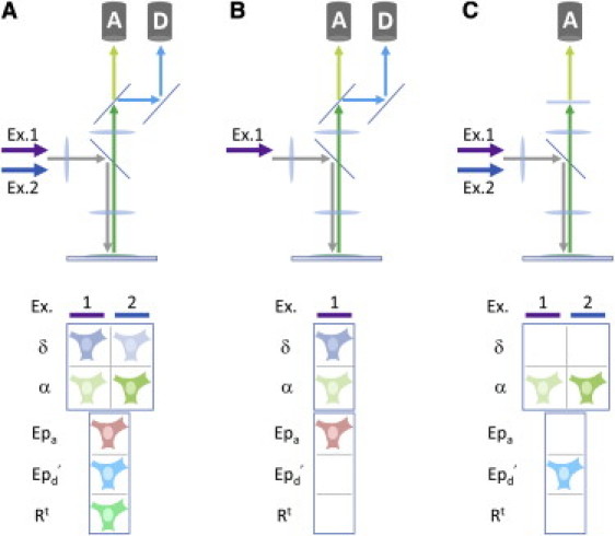
The microscope configurations required for the presented analysis methods. Different analysis methods can be used depending on the microscope configuration. For each configuration, a set or subset of apparent concentrations, δ⁽ⁱ⁾ and α⁽ⁱ⁾, can be measured and used differently by the proposed methods to determine certain lux-FRET quantities. (A) In the dual excitation wavelength/spectrally resolved emission channels configuration, enough parameters are measured to use any method introduced to determine Ep_a, Ep′_d , and the total concentrations, as well as their ratio R^t. It should be noted that Ep_a determined from Methods II and IV (α⁽²⁾/δ⁽¹⁾) and R^t can only be quantified in this configuration. (B) In the single excitation wavelength/spectrally resolved emission channels configuration, high temporal resolution measurements of Ep_a can be performed using Method III (α⁽¹⁾/δ⁽¹⁾). This method requires that R^t has already been measured and assumed to be invariant. This configuration is also widely used for ratiometric measurements. (C) The dual excitation wavelength/single emission channel configuration can be used to determine Ep′_d through Methods I and V (α⁽¹⁾/α⁽²⁾), both of which require the determination of R_TC from a tandem construct reference.

In many intermolecular investigations and essentially all intramolecular investigations, the spatial distribution of the ratio of donor and acceptor molecules is not expected to change, apart from possible differential bleaching. In such cases, it is possible to quantify the apparent FRET efficiency with only a fraction of the information obtained during the dual wavelength excitation/spectrally resolved emission measurements, as outlined below.

Single wavelength excitation/spectrally resolved emission

Method III (α⁽¹⁾/δ⁽¹⁾) can be performed using Eq. 3a with a single excitation wavelength and spectrally resolved emission channels as depicted in Fig. 1 B, if the quantity R^t has been measured and is assumed to be invariant. The use of a single excitation wavelength increases the temporal resolution of a dynamic Ep_a measurement, such that it is only limited by the acquisition rate of the equipment used.

Dual wavelength excitation/single emission channel

Equations 1 and 7, used in Methods I and V (α⁽¹⁾/α⁽²⁾), do not contain apparent donor concentrations but only those of acceptors, measured at two excitation wavelengths. The additional parameters are calibration constants. This means that one can determine the product $E{p}_d^{\prime }$ (or else $E{f}_a{p}_d^{\prime }$ for a measurement of intermolecular FRET) with a single emission window in the range of acceptor fluorescence, using alternating dual excitation (outlined by Fig. 1 C), if donor bleedthrough into the emission channel is negligible. If there is significant donor bleedthrough, it is possible to use information from an initial dual wavelength excitation/spectrally resolved measurement to determine $E{p}_d^{\prime }$ as a function of the total fluorescence including donor bleedthrough (see the Supporting Material). If such alternating excitation is available, the measurements are very conveniently performed with a standard camera or photometric device, because they do not require switching of beamsplitters and emission filters.

For many FRET experiments, the donor/acceptor ratio, R^t, is constant (apart from differential bleaching). For the dynamic FRET-measurements outlined above, it is advisable to determine it once before a measurement series and once afterwards, to check for constancy or else reveal differential bleaching effects.

Noise propagation

Under the conditions of the measurements presented below, the noise of fluorescence signals is dominated by shot noise, which for Poisson statistics leads to the following expression for the variance of the fluorescence reading in wavelength channel k:

$$Var\left(F\left({\lambda }_k\right)\right)=s’F\left({\lambda }_k\right)+{\sigma }_{o,k}^2.$$ (8)

Here s′ is the apparent peak amplitude of the single photon signal and σ²_o,k is the background noise of channel k. For simplicity, we assume s′ to be wavelength-independent, which is sufficient for most experiments (see the Supporting Material), although photophysics would predict this to be inversely proportional to wavelength (see (12) for a treatment, which includes wavelength dependence). The variance of the derived quantities α⁽ⁱ⁾ and δ⁽ⁱ⁾ can either be calculated from Var(F(λ_k)) (see the Supporting Material) or else measured as a function of excitation intensity.

For the analysis of the expected noise of Ep_a and $E{p}_d^{\prime }$, as defined by Eqs. 1–3 and 7 we consider calibration constants and the quantity R^t to be constant and we use Gaussian error propagation. We provide the equations for the square of the coefficient of variation (CV² = Var/Mean²), which yield simple expressions (see the Supporting Material for the derivations) and in the results sections we mostly use the square of the signal/noise ratio (SNR²), which is the inverse of CV².

For Method I,

$$C{V}_{E{p^{\prime }}_d}^2=\frac{{\left({\alpha }^{\left(1\right)}\right)}^2{\left({\alpha }^{\left(2\right)}\right)}^2{\left(\Delta r\right)}^2}{{\left({\alpha }^{\left(1\right)}{r}^{\text{ex},\left(2\right)}-{\alpha }^{\left(2\right)}{r}^{\text{ex},\left(1\right)}\right)}^2{\left({\alpha }^{\left(2\right)}-{\alpha }^{\left(1\right)}\right)}^2}\left(C{V}_{{\alpha }^{\left(1\right)}}^2+C{V}_{{\alpha }^{\left(2\right)}}^2\right).$$ (9)

For Method II,

$$C{V}_{E{p}_a}^2=\frac{{\left(\Delta r\right)}^2{\left({\delta }^{\left(1\right)}\right)}^2}{{\left(\Delta \alpha \right)}^2{\left(\Delta r{\delta }^{\left(1\right)}+\Delta \alpha \right)}^2}\left(\mathrm{var}\left({\alpha }^{\left(1\right)}\right)+\mathrm{var}\left({\alpha }^{\left(2\right)}\right)+{\left(\Delta \alpha \right)}^{2}C{V}_{{\delta }^{\left(1\right)}}^2\right).$$ (10)

For Method III (α^(1)/δ⁽¹⁾),

$$C{V}_{E{p}_a}^2=\frac{{\left({\alpha }^{\left(1\right)}\right)}^2{\left({\delta }^{\left(1\right)}\right)}^2{\left(r^{\text{ex},1}+R^t\right)}^2}{{\left({\alpha }^{\left(1\right)}+{\delta }^{\left(1\right)}{r}^{\text{ex},1}\right)}^2{\left({\alpha }^{\left(1\right)}-{\delta }^{\left(1\right)}{R}^t\right)}^2}\left(C{V}_{{\alpha }^{\left(1\right)}}^2+C{V}_{{\delta }^{\left(1\right)}}^2\right).$$ (11a)

For Method IV (α^(2)/δ⁽¹⁾),

$$C{V}_{E{p}_a}^2=\frac{{\left({\alpha }^{\left(2\right)}\right)}^2{\left({\delta }^{\left(1\right)}\right)}^2{\left(r^{\text{ex},2}+R^t\right)}^2}{{\left({\alpha }^{\left(2\right)}+{\delta }^{\left(1\right)}{r}^{\text{ex},2}\right)}^2{\left({\alpha }^{\left(2\right)}-{\delta }^{\left(1\right)}{R}^t\right)}^2}\left(C{V}_{{\alpha }^{\left(2\right)}}^2+C{V}_{{\delta }^{\left(1\right)}}^2\right).$$ (11b)

For Method V (α^(1)/α⁽²⁾),

$$C{V}_{E{p}_d}^2=\frac{{\left({\alpha }^{\left(1\right)}\right)}^2}{{\left({\alpha }^{\left(1\right)}-{\alpha }^{\left(2\right)}\right)}^2}\left(C{V}_{{\alpha }^{\left(1\right)}}^2+C{V}_{{\alpha }^{\left(2\right)}}^2\right).$$ (12)

For the measurements of the emission ratio, the CV² is simply the sum of the CV² values of the numerator (F^1,2) and the denominator (F^1,1). Ligand concentration can be estimated from the emission ratio measurements (6) as well as from FRET measurements (see the Supporting Material). The estimated variance of ligand concentration computed from FRET efficiency is

$$C{V}_{\left[X\right]}^2={\left(\frac{E}{\left(E-E_o\right)}·\frac{\left(E_{\max }-E_0\right)}{\left(E_{\max }-E\right)}\right)}^{2}C{V}_E^2,$$ (13)

and from emission ratio measurements,

$$C{V}_{\left[X\right]}^2={\left(\frac{R}{\left(R-R_o\right)}·\frac{\left(R_{\max }-R_0\right)}{\left(R_{\max }-R\right)}\right)}^2\left(C{V}_{F_1}^2+C{V}_{F_2}^2\right).$$ (14)

Materials and Methods

Adherent cell culture and transfection

HEK293 cells from the American Type Culture Collection (ATCC, Manassas, VA) were grown in Dulbecco's modified Eagle's medium containing 10% fetal calf serum and 1% penicillin/streptomycin at 37°C under 5% CO₂. For transient transfection, cells were seeded at low density on 10-mm or 25-mm coverslips (∼1 × 10⁵ or ∼5 × 10⁵, respectively) and transfected with appropriate vectors using Lipofectamine 2000 Reagent (Invitrogen, Carlsbad, CA) according to the manufacturer's instruction. Four hours after transfection, cells were serum-starved overnight before analysis. The CFP-YFP tandem construct has been described previously in Wlodarczyk et al. (8). The CFP-EPAC-YFP construct was presented in Ponsioen et al. (4).

Live cell lux-FRET imaging

All images were acquired on a LSM 510 Meta confocal microscope (Carl Zeiss, Jena, Germany) with a 40× oil-immersion objective (NA 1.3). For excitation of CFP, the 458-nm line of a 40-mW Argon laser was used with a 458-nm dichroic mirror and emission was collected through a 170-μm confocal pinhole over eight channels spanning 464–636 nm. For excitation of YFP, the 488-nm laser line of the Argon laser was used with a 488-nm dichroic mirror with the emission window shifted from 497 nm to 583 nm. The excitation intensity was set such that SNR of the measurement was maximized within the constraint that bleaching of either fluorophores did not exceed ∼0.5% per acquisition. The scanning pixel dwell time was set to 12.8 μs and the detector gain to 550 V. All images were digitized/collected with 12-bit resolution.

For dynamic measurements of the Epac FRET sensor, coverslips were placed in a custom-made chamber with 500 μL of D-PBS. Image acquisitions with excitation at 488 nm preceded and followed a series of 61 images acquired at 10-s intervals with excitation at 458 nm. After the 20th image acquisition, forskolin was added to a final concentration of 10 μM.

Lux-FRET image analysis

All analysis was performed using MATLAB 7.2 (The MathWorks, Natick, MA). Before two-excitation lux-FRET analysis, images were brought into register by shifting one image to minimize the summed squared difference of the normalized images. This usually required <2 pixel shift in the x-y plane. Next, linear unmixing, with nonnegativity constraints, was performed pixel by pixel using background-subtracted reference and FRET sample spectra. The reference spectra were obtained from user-selected regions of interest (ROI) of images of cells expressing either donor or acceptor that were acquired with the same settings as the FRET sample. The apparent concentrations resulting from the linear unmixing were then used according to Eqs. 1–3 and 7 to calculate apparent FRET efficiencies.

Results

FRET Imaging of an Epac-based cAMP sensor

Two sets of confocal images of N1E-115 cells expressing a CFP-Epac-YFP FRET sensor were acquired with 458-nm and 488-nm excitation, respectively, each over eight emission channels. These images were first brought into register. Then the apparent concentrations of CFP and YFP at each pixel were determined by nonnegative linear unmixing using previously determined reference spectra. With these apparent concentrations, as well as some calibration constants, the lux-FRET quantities defined in Eqs. 1–3 and 7 were computed, resulting in images representing the spatial distribution of these quantities. A ratiometric FRET estimator, the 550/485-nm emission ratio, was also computed for the 458-nm excitation using the summed emission collected in the first two channels to approximate that collected through a 485±21.5-nm filter and the summed fourth and fifth channel to approximate that collected through a 550±21.5-nm emission filter. Fig. 2 illustrates the results. The left columns (Fig. 2, A and B) represent the raw data, which are the sum of the emissions obtained in the two excitations (Fig. 2 A, top panel) and the 550/485-nm emission ratio derived in a way similar to that of Miyawaki et al. (5) (Fig. 2 B, lower panel).

Figure 2.

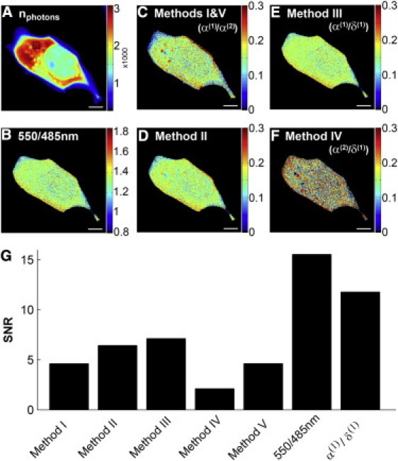
Comparison of image analysis methods. Confocal images of N1E-115 cells expressing an EPAC-based cytosolic cAMP FRET sensor were analyzed with the various lux-FRET and ratiometric methods. (A) The number of photons detected during a sequence of two excitations. This number detected within the ROI, shown as a black box, was found to be 2876 photons per pixel. (B) The YFP/CFP emission ratio was estimated as the ratio of emission in the 550±21.5-nm and 485±21.5-nm spectral windows. (C) Using information from two image acquisitions, with excitation wavelengths 458 nm and 488 nm, Ep′_d was calculated using Method I or V (α^(1)/α⁽²⁾); the two are equivalent. (D) Ep_a was calculated from dual excitation measurements according to Method II. (E) Ep_a was calculated from a single acquisition using Method III (α^(1)/δ⁽¹⁾), and R^t as a calibration constant. (F) Ep_a was also calculated from the two-excitation wavelength measurement using Method IV (α^(2)/δ⁽¹⁾). To allow for comparison of the lux-FRET quantities to the ratiometric measurement, the color scales were adjusted appropriately. Scale bars represent 5 μm. (G) The SNR measured from corresponding ROIs of the quantities imaged in panel A are shown. Also included is the SNR of the apparent concentration ratio α⁽¹⁾/δ⁽¹⁾. The 550/485-nm ratio provides the most favorable SNR, while the lux-FRET quantity with the most favorable SNR is Ep_a calculated using Method III (α⁽¹⁾/δ⁽¹⁾).

The total emission is expressed in terms of the number of collected photons by dividing the fluorescence intensity by the apparent single photon signal, s′, derived from Eq. 8 (also see the Supporting Material). Fig. 2 C, top panel of the center column, shows the quantity Ep′_d, calculated according to Method I or Method V (α⁽¹⁾/α⁽²⁾) (the two are equivalent). These quantities are based on the measurement of acceptor fluorescence only, comparing sensitized emission (α⁽¹⁾) with directly excited emission (α⁽²⁾). It is quite obvious that these images are somewhat noisier than the images of the emission ratio. The bottom panel of the center column, Fig. 2 D, shows the quantity Ep_a according to Method II. The right column shows Ep_a according to Method III (α⁽¹⁾/δ⁽¹⁾) (Fig. 2 E, top panel) and Method IV (α⁽²⁾/δ⁽¹⁾) (Fig. 2 F, bottom panel). The result of Method III (α⁽¹⁾/δ⁽¹⁾) is very similar to the simple emission ratio (Fig. 2 B), except that it is calibrated in terms of Ep_a and that the emissions have been obtained by spectral decomposition rather than from two suitable spectral windows. The SNR is better than that of the acceptor-based analysis (Method I or V (α⁽¹⁾/α⁽²⁾), Fig. 2 C) but not quite as good as that of the plain ratio. Finally Method IV (α⁽²⁾/δ⁽¹⁾), illustrated in Fig. 2 F, calculates the ratio of directly excited acceptor emission over directly excited donor emission. It is apparent that this method results in the lowest SNR and also introduces some bias.

In the images produced from analysis methods that require information from two excitations (Fig. 2, C, D, and F), there are frequent edge effects due to slight, often subpixel, misregistration. Apart from that, the mean FRET efficiency is reasonably uniform throughout the entire cell. However, as will be discussed in greater detail later, the noise varies between regions due to differences in the amount of the sensor and the number of collected photons.

Fig. 2 G provides a quantitative analysis of the SNR of the images of Fig. 2, A–F. A small region of interest was selected (shown as a black box in Fig. 2 A) and the mean of pixel values as well as the variance between pixels was calculated. Subsequently the signal/noise ratio was determined. This is a dimensionless and scale-invariant quantity. It allows us to directly compare the level of noise present in each measurement, if the quantities analyzed are sufficiently constant over the ROI. The mean estimated per-pixel photon count (Fig. 2 A) within the selected ROI is 2876 photons (see Materials and Methods). Although the signal is not completely uniform within this ROI, the nonuniform concentration should not affect the variance measurement for the derived quantities because they involve only ratios of two quantities, each of which scales with signal strength. The SNR values sampled from the quantities illustrated in Fig. 2, A–F, are compared in Fig. 2 G. This shows, as was concluded from Fig. 2, A–F, that Method III (α⁽¹⁾/δ⁽¹⁾) provides the best SNR of the lux-FRET quantities and that the 550/485-nm emission ratio provides the overall best SNR in this example. Differences between the different analysis modes will be addressed in the Discussion.

Dependence of SNR² of FRET estimators on the total number of detected photons and FRET efficiency

To develop the relationship between the SNR² of our lux-FRET quantities and the excitation intensities, we performed multiple measurement of a CFP-YFP tandem construct at varied excitation intensities. The measured SNR² of the apparent concentrations, α⁽¹⁾, α⁽²⁾, and δ⁽¹⁾, were fit as linear functions of the estimated number of detected photons.

We then performed a thought-experiment, in which we took the values for δ⁽¹⁾ and α⁽ⁱ⁾ from the measurement shown in Fig. 2 (with an Ep_a of 0.16, n₁ = 1430 photons collected in excitation 1 and n₂ = 1445 photons collected in excitation 2) and calculated the SNR² values according to Eq. 10. We simulated changes in excitation intensity by varying proportionally the number of photons collected. In these calculations we assumed δ⁽¹⁾ and α⁽ⁱ⁾ values to be constant (because they are normalized for intensity changes) and their CV² values to vary according to the above-mentioned linear fitting.

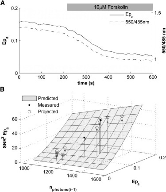
The results are shown in Fig. 3 A. As would be expected, the SNR² of Ep_a determined from Method II increases with the number of detected photons for both excitations. Interestingly, this figure suggests that the number of photons collected during the respective excitations do not contribute equally to the SNR of Ep_a. The contour plotted across the surface in Fig. 3 A represents the predicted SNR² of Ep_a for all measurements, in which a total of 2876 photons are collected during the two excitations. The maximum of this contour, illustrated as the point atop the solid vertical line, occurs when ∼66% of the total photons are collected during the 458-nm excitation. The open circle, together with the dotted vertical line, represents the measured SNR² of Ep_a sampled from Fig. 2 D. In that experiment, only 50% of total photons were collected during the short wavelength. Fig. 3 A suggests that the SNR² of Ep_a could have been improved by ∼15% by increasing excitation 1 at the expense of excitation 2. There is a second reason why it may be advantageous to use lower intensity in the long wavelength excitation, particularly at high FRET efficiencies. This relates to the fact that the acceptor is subject to bleaching during both excitations and, therefore, its bleaching may be limiting. This point will be addressed in more detail in the Discussion.

Figure 3.

Dependence of SNR² of FRET estimators on the total number of detected photons and FRET efficiency. Fluorescence data were obtained using a CFP-YFP tandem construct and expectations for the SNR² were calculated from the error propagation analysis. (A) SNR² of the two-excitation-dependent Ep_a calculated using Method II with error propagation calculated using Eq. 10. The contour plotted across the surface in Fig. 3A represents the predicted SNR² of Ep_a for all measurements in which a total of 2876 photons are collected during the two excitations. The maximum of this contour (see point atop the solid vertical line) occurs when ∼66% of the total photons are collected during the 458-nm excitation. (Open circle with dashed vertical line) SNR² of Ep_a measured when 50% of the 2876 photons were collected during the short wavelength excitation. (B) Comparison of the SNR² of Ep_a determined from Method III (α^(1)/δ⁽¹⁾) and the SNR² of the 550/485-nm emission ratio for different FRET efficiencies and numbers of detected photons. These results show that the SNR² of the ratiometric measurement exceeds that of the lux-FRET quantity for the FRET efficiencies expected from most FRET sensors. However, this figure proposes that at relatively high FRET efficiencies, above ∼0.38, the SNR² of Ep_a will begin to exceed that of the 550/485-nm ratio.

To determine the effect of changes in FRET efficiency on the SNR² of the measurements, we estimated the SNR² for the hypothetical case in which the FRET efficiency of a sensor changes at constant total acceptor/donor ratio. To do so, we used Eq. 27 from Wlodarczyk et al. (8), to calculate the apparent concentrations expected for a given FRET value. The same linear relationship between SNR² values of the apparent concentrations and the number of collected photons, as above, was used (this neglects small changes in noise, which may result from variable degrees of spectral overlap). Fig. 3 B illustrates the relationship between the SNR² of Ep_a (Method III (α^(1)/δ⁽¹⁾)) and the total number of detected photons as a shaded semitransparent surface with a black grid. The same relationship for the SNR² of the 550/485-nm emission ratio measurement is illustrated as a semitransparent dark-shaded surface with a white grid. We present these two quantities because they were found to have the highest SNR² (Fig. 2 G) and because they can both be determined from single excitation measurements. The figure clearly shows that the SNR² of both Ep_a and the ratio increase with an increase in the number of photons detected. For the majority of the figure, the SNR² of the 550/485 ratio is greater than that of Ep_a. However, at relatively high FRET efficiency, >∼38%, the SNR² of Ep_a begins to exceed that of the ratio.

Time series measurements of select FRET estimators

As previously mentioned, Method III (α^(1)/δ⁽¹⁾) and the 550/485-nm emission ratio only require a single excitation acquisition, making them especially well suited for measuring dynamic changes in FRET. It should be reiterated that this method does require the knowledge of R^t, which can only be obtained by a two-excitation measurement (see Eq. 27 in Wlodarczyk et al. (8)). R^t, the ratio of total donor and total acceptor concentration, should, however, be constant for a given tandem construct, except for possible differential bleaching. Therefore, in order to check for such consistency, we performed two-excitation measurements preceding and after multiple single excitation measurements, as described in Materials and Methods. Fig. 4 illustrates such a measurement performed on the same cells expressing the CFP-EPAC-YFP cAMP sensor, as shown in Fig. 3. Forskolin, a membrane-permeable activator of adenylyl cyclase, was applied at a final concentration of 10 μM at t = 200 s. The increase in [cAMP] resulting from the forskolin-induced activation of adenylyl cyclase is shown in Fig. 4 A as a decrease in the measured Ep_a from ∼0.16 to 0.05 (dark trace, left ordinate). Correspondingly, the decrease in donor quenching and acceptor sensitization results in a decrease in the 550/485-nm emission ratio from ∼1.33 to 0.98 (light trace, right ordinate).

Figure 4.

Time course of Ep_a and the 550/485-nm emission ratio. Multiple single excitation measurements of cells expressing the CFP-EPAC-YFP cAMP sensor shown in Fig. 2 were performed after an initial two-excitation measurement. Forskolin was applied to a final concentration of 10 μM at t = 200 s. (A) The values calculated for Ep_a determined from Method III (α⁽¹⁾/δ⁽¹⁾) and the 550/485-nm ratio are plotted over time (dark and light lines, respectively). Note the different scales for the two quantities. (B) Twelve points were sampled, in 50-s intervals, from the Ep_a measurements presented in panel A. The SNR² of these measurements were plotted (solid points) against the corresponding FRET efficiency and number of detected photons. (Shaded surface) Subsection of the surface presented in Fig. 3B, representing the relationship among SNR² of Ep_a, FRET efficiency, and number of detected photons as predicted from the error propagation analysis. (Open circles) Projection of each sampled measurement onto the prediction surface.

In this example, the initial R^t, which is used as a calibration constant throughout the time series, equals 1.82. The value of R^t computed after the time series equaled 1.66, suggesting relatively little differential bleaching. The total acceptor concentration, [A^t], changed from 0.67 to 0.53, indicating that ∼20% of the 69% change measured in Ep_a results from acceptor bleaching. The total donor concentration changed from 0.37 to 0.32 throughout the course of the measurement and only influenced Ep_a indirectly through the differential bleaching present in R^t.

Effect of FRET change and bleaching on Ep_a and its SNR²

During the course of the measurement shown in Fig. 4 A, not only is there a decrease in FRET efficiency resulting from the increase in [cAMP], but there is also a gradual decrease in the number of detected photons resulting from the photobleaching of both the donor and acceptor fluorophores. Intuitively, both of these factors will contribute to a decrease in the SNR² of Ep_a. The error propagation analysis presented in Fig. 3 allows one to predict this effect. In Fig. 4 B, a subsection of the SNR² Ep_a surface in Fig. 3 B is presented as a light-gray semitransparent surface with a black grid. The solid black points in this figure represent the measured SNR² of Ep_a at the corresponding values of Ep_a and mean detected photons. The open circles represent the projection of each sampled measurement onto the prediction surface. Twelve equally spaced samples from the time course measurement are plotted to illustrate the trend. This figure shows that the decrease both in FRET efficiency and in the number of detected photons, over time, results in a decreased SNR² of Ep_a that is quite well predicted by theory.

Estimation of cAMP concentration

Measurements, such as those presented thus far, are often used only to indicate relative changes in the concentration of a ligand, in this case [cAMP]. However, it is possible to estimate the absolute ligand concentration from measurements, if the maximum and minimum FRET efficiencies (E_max and E_o), corresponding to the sensor in its free and bound states are known, together with the Hill coefficient and the dissociation constant. Likewise, [cAMP] can be calculated from the simple emission ratio, if the corresponding maximum and minimum ratios are known (see (6) and the Supporting Material). For the following discussion we assume, for simplicity, that p_a,d = 1 and bleaching is negligible. From the supplemental information provided by Ponsioen et al. (4), we know that the Hill coefficient, n, is ∼1 and that we can expect an ∼70% decrease from the initial FRET value during application of 10 μM forskolin. Assuming low basal [cAMP] and near-saturation of the sensor with application of forskolin, we can approximate, for example, that E_free = 0.165 and E_bound = 0.015. The corresponding 550/485-nm ratios expected from the microscope used are R_free = 1.40 and R_bound = 0.85 (see the Supporting Material for the conversion from E to R). The error propagation resulting from the conversion of FRET efficiency into ligand concentration is described by Eq. 13. Equation 14 describes the error propagation resulting from the conversion of emission ratio into ligand concentration. Maps of [cAMP]/K_d were computed from the Ep_a and 550/485-nm ratio maps. Literature values for the K_d of this construct vary greatly (4,13), so no absolute estimate was made. From now on, [cAMP]/K_d will be designated as [cAMP]^∗. The SNR² was calculated as previously discussed.

The mean [cAMP]^∗ can be calculated in two ways. We can either convert individual pixel values from Ep_a (or 550/485-nm) to [cAMP]^∗ and subsequently take the average of the ROI or we can take the mean Ep_a (or 550/485 nm) and convert it to [cAMP]^∗. In Fig. 5 A we show the time course of [cAMP]^∗ calculated by the latter strategy. The solid line represents the [cAMP]^∗ calculated from the mean Ep_a and the dotted line represents that calculated from the mean 550/485-nm emission ratio. Both these traces show an increase in [cAMP] to ∼3.7-fold the K_d value. In Fig. 5 B we show the SNR² of [cAMP]^∗ using the former strategy in which individual per-pixel values of [cAMP]^∗ are calculated from Ep_a (solid trace) and from 550/485 nm (dotted trace). This figure shows that the SNR² begins to increase as the emission ratio or Ep_a begins to diverge from the ligand free value, as Eqs. 13 and 14 would suggest. However, over time the SNR² of [cAMP]^∗ decreases dramatically due to bleaching, the decrease in FRET efficiency, and convergence upon the fully bound FRET estimator value. Interestingly, even though the SNR² of the 550/485-nm ratio is significantly greater than that of Ep_a according to Fig. 2, the SNR² of the [cAMP]^∗ estimation from these two quantities are essentially equivalent.

Figure 5.

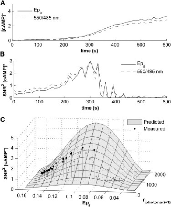
Time course of the estimated cAMP concentration. With the knowledge of certain calibration parameters the absolute ligand concentration can be readily calculated. (A) (Solid line) [cAMP]^∗ calculated from the mean Ep_a (Method III (α⁽¹⁾/δ⁽¹⁾)) and (dotted line) [cAMP]^∗ calculated from the mean 550/485-nm emission ratio. (B) (Dark and light lines) SNR² of the per pixel [cAMP]^∗ values based on Ep_a and 550/485-nm emission ratio, respectively, over time. (C) (Shad surface) Relationship among the SNR² of the [cAMP]^∗, the FRET efficiency of the sensor, and the number of detected photons. (Solid points) Individual estimates from the measurements of the time series. This figure shows, similarly to Fig. 4B, that the error propagation model accurately predicts the expected SNR².

Fig. 5 C shows the relationship among the number of detected photons, the FRET efficiency of the sensor, and the SNR² of the [cAMP]^∗ estimate, derived from our error propagation analysis. The solid points indicate the individual values of our measurement. This figure shows, similarly to Fig. 4 B, that our error propagation model accurately predicts the expected SNR². It clearly shows the increase in SNR² of the [cAMP]^∗ estimate because the FRET efficiency decreases from that of the ligand free state. As Eq. 13 suggests, this figure also shows that the SNR² (1/CV²) decreases dramatically when FRET efficiency begins to approach that of the bound state. Also, as would be expected, the model indicates the coordinated decrease of the SNR² of [cAMP]^∗ with that of the number of detected photons.

Regarding these results, it should be pointed out that the variance of the fluorescence readings and that of the ratios varies only little during the course of these measurements. The major reason for the dramatic decrease in signal/noise ratio lies in the fact that, at both ends of the dynamic range of the sensor, small changes in the signal are converted into large changes in the derived quantity. The noise divided by the dynamic range of these two [cAMP] estimators are very similar to each other, and decreases only slightly in proportion to bleaching.

Discussion

FRET-based sensors have become invaluable tools in the characterization of spatial and temporal dynamics of a large number of cellular signaling processes. The utility of these sensors, however, is limited by the noise inherent in photon statistics as well as in their detection above an autofluorescence background. The noise is propagated through the ratio measurements often used to identify FRET. More complex analysis procedures, which aim at a quantitative analysis of FRET efficiency, introduce additional noise. The value of FRET sensors is further compromised due to the fact that their sampling is an inherently destructive process. Photobleaching limits the total number of photons that can be collected from a sample. Thus, the efficient use of the available photons must be carefully considered to optimize the information retrieved from the system being investigated.

In this study, we have explored the propagation of photon and detection noise through the equations often used to analyze fluorescence collected from FRET sensors. We have pointed out that FRET estimators can be calculated from any ratio of the three apparent fluorophore concentrations of a lux-FRET measurement and we have developed models relating the signal/noise ratio of such estimators to the number of photons collected. We further explored the dependence of the lux-FRET quantity, Ep_a, on the number of photons collected in each respective acquisition. This allows us to refine the rule-of-thumb for noise optimization mentioned in the Introduction. The preliminary conclusion had been that one should maximize the number of photons (within the limits of bleaching) collected in the two measurements, which are used in a given analysis mode. We can add to that how error propagation usually leverages noise, when calculating derived parameters, such as FRET efficiency or the concentration of a ligand. The best performing lux-FRET analysis mode was found to be the mode based on the emission ratio after donor excitation (Eq. 3, i = 1), which is quite similar to the standard emission ratio method. Surprisingly the analysis mode, which is based on the two best-resolved signals, δ⁽¹⁾ and α⁽²⁾, performed very poorly (Fig. 2, F and G) due to very unfavorable error propagation.

A close look at Fig. 3 A indicates that aiming at equal numbers of collected photons during the two excitations does not provide for optimal SNR² of Ep_a. The majority of the photons collected in the long-wavelength acquisition are emitted from the acceptor, such that this signal is minimally degraded by spectral overlap. During the short-wavelength excitation, however, both donor and acceptor molecules significantly contribute to emission and the spectral unmixing of their contributions leads to a loss of information. This suggests that an optimum SNR² for Ep_a would be achieved by detecting more photons in the short-wavelength acquisition at the expense of photon detection during the long-wavelength acquisition. In Fig. 3 A, we demonstrate that at the optimum SNR² of Ep_a, ∼66% of the total photons would be collected during the short-wavelength acquisition. The SNR² of Ep_a, corresponding to the measurement illustrated in Fig. 2 D, is ∼44 and was achieved with only 50% of the total photons being collected during the short wavelength excitation. Fig. 3 A suggests that a SNR² of Ep_a = 59 could be achieved by altering excitation intensities such that we move to the maximum of the contour.

The use of lower intensity in the long wavelength excitation, particularly at high FRET efficiency, is also advantageous when considering the effects of photobleaching. Due to the combination of direct and sensitized excitation of the acceptor during the short-wavelength excitation measurement and its direct excitation during the long-wavelength excitation, its photobleaching will almost certainly be limiting. This holds both for the dual excitation methods outlined above, as well as for other methods such as the three-filter cube. Unfortunately, bleaching of the acceptor not only results in a decrease in total emission and thus in the SNR² of the computed quantities, but it also decreases Ep_a and the 550/485-nm emission ratio. These changes can easily be misinterpreted as changes in the concentration of the ligand being assayed. By reducing the intensity of the long-wavelength excitation, the user can find a reasonable compromise between optimizing SNR and minimizing of the effect of acceptor bleaching. Except for very photostable acceptors and very low FRET efficiencies, the acceptor will usually be more susceptible to bleach than the donor. Therefore, in many cases optimum conditions are obtained with relatively low excitation intensities at the long wavelength (see below). It should be noted that this compromise is also influenced by the relative photostability of the chromophores used as well as their FRET efficiencies. In our experiments with the FRET pair CFP and YFP and at FRET efficiencies at ∼0.15, we found that such a compromise is reached when 60–70% of all photons are collected during the short-wavelength excitation. Excitation wavelength has also been suggested to influence the SNR of FRET estimators (14). Simulations show that the SNR of the FRET estimators investigated is maximized when the short and long wavelength exposures selectively excite donor and acceptor molecules, respectively (data not shown).

When comparing the investigated lux-FRET and ratiometric quantities we identified two analysis modes, which were especially well suited for measuring dynamic changes in FRET efficiency: The 550/485-nm emission ratio and the lux-FRET quantity, Ep_a derived from Eq. 3 with i = 1. These two methods had the highest SNR² and they can be performed with a single excitation. Through the error propagation analysis, we show that the SNR² of ratiometric measurements exceeds that of the lux-FRET quantities for the expected FRET efficiencies of most FRET sensors. Interestingly, our analysis suggests that above E ∼ 0.38, the SNR² of Ep_a will begin to exceed that of the 550:485-nm ratio. We performed a time series of measurements of a CFP-Epac-YCP FRET sensor during an increase in intracellular cAMP concentration after the activation of adenylyl cyclase. Both analysis modes similarly reported the relative change in the ratio of free and bound sensors. We also show that the SNR² of Ep_a measured during this experiment is quite well described by the predictions of the error propagation analysis, both with respect to the change in FRET efficiency and regarding the decrease in the number of detected photons.

The ultimate utility of the measurements of Ep_a or the 550/485-nm emission ratio is to provide an estimation of the absolute ligand concentration. This conversion can be readily performed with the appropriate calibration information; however, it further amplifies errors. An interesting finding of this investigation was that, although the SNR² 550/485 nm exceeds that of the SNR² of Ep_a, these two quantities perform similarly when estimating the absolute ligand concentration. The SNR² of the ligand concentration determined by these two methods was found to be essentially equal, suggesting that the error propagation through Eq. 13 is more favorable than through Eq. 14. Overall, however, the SNR² of both estimates of ligand concentration are much lower than those of the raw FRET signals. It should also be noted that ratiometric measurements are generally instrument-dependent and that the calibration required for absolute ligand concentration measurements may not be trivial to perform on all instruments. Quantitative estimates of FRET efficiency, however, are not instrument-dependent. Because these two analysis modes perform similarly in estimating the absolute ligand concentration, the use of Ep_a is advantageous when cross-platform calibration is required.

The levels of noise in the presented data may seem excessive. However, it should be noted that the images used in this investigation were acquired near confocal resolution (lateral and axial) without any frame or line averaging. One way in which the quality of the FRET estimates could have been improved is by opening the confocal pinhole to allow for the collection of significantly more photons during a given excitation. Of course, the collection of additional photons would come at the cost of lateral, and to a greater extent, axial resolution. Likewise, low-pass filtering or spatial Gaussian blurring will considerably decrease the level of noise. These, however, also compromise the resolution.

The analysis presented in this investigation provides guidelines for the selection of optimal parameters for FRET measurements. It allows us to predict how the quality of our measurements will change with the expected changes in FRET efficiency and with the decrease in the number of detected photons due to progressive photobleaching of the sensor. Collection of this information, in preliminary measurements, allows for the selection of sampling parameters that will ensure an acceptable SNR over the time course required to characterize the dynamics of a given change in FRET.

References

- 1.Miyawaki A., Llopis J., Tsien R.Y. Fluorescent indicators for Ca2+ based on green fluorescent proteins and calmodulin. Nature. 1997;388:882–887. doi: 10.1038/42264. [DOI] [PubMed] [Google Scholar]
- 2.Sakai R., Repunte-Canonigo V., Knöpfel T. Design and characterization of a DNA-encoded, voltage-sensitive fluorescent protein. Eur. J. Neurosci. 2001;13:2314–2318. doi: 10.1046/j.0953-816x.2001.01617.x. [DOI] [PubMed] [Google Scholar]
- 3.Seth A., Otomo T., Rosen M.K. Rational design of genetically encoded fluorescence resonance energy transfer-based sensors of cellular Cdc42 signaling. Biochemistry. 2003;42:3997–4008. doi: 10.1021/bi026881z. [DOI] [PubMed] [Google Scholar]
- 4.Ponsioen B., Zhao J., Jalink K. Detecting cAMP-induced Epac activation by fluorescence resonance energy transfer: Epac as a novel cAMP indicator. EMBO Rep. 2004;5:1176–1180. doi: 10.1038/sj.embor.7400290. [DOI] [PMC free article] [PubMed] [Google Scholar]
- 5.Miyawaki A., Griesbeck O., Tsien R.Y. Dynamic and quantitative Ca2+ measurements using improved cameleons. Proc. Natl. Acad. Sci. USA. 1999;96:2135–2140. doi: 10.1073/pnas.96.5.2135. [DOI] [PMC free article] [PubMed] [Google Scholar]
- 6.Grynkiewicz G., Poenie M., Tsien R.Y. A new generation of Ca2+ indicators with greatly improved fluorescence properties. J. Biol. Chem. 1985;260:3440–3450. [PubMed] [Google Scholar]
- 7.Hoppe A., Christensen K., Swanson J.A. Fluorescence resonance energy transfer-based stoichiometry in living cells. Biophys. J. 2002;83:3652–3664. doi: 10.1016/S0006-3495(02)75365-4. [DOI] [PMC free article] [PubMed] [Google Scholar]
- 8.Wlodarczyk J., Woehler A., Neher E. Analysis of FRET signals in the presence of free donors and acceptors. Biophys. J. 2008;94:986–1000. doi: 10.1529/biophysj.107.111773. [DOI] [PMC free article] [PubMed] [Google Scholar]
- 9.Erickson M.G., Alseikhan B.A., Yue D.T. Preassociation of calmodulin with voltage-gated Ca2+ channels revealed by FRET in single living cells. Neuron. 2001;31:973–985. doi: 10.1016/s0896-6273(01)00438-x. [DOI] [PubMed] [Google Scholar]
- 10.Shaner N.C., Steinbach P.A., Tsien R.Y. A guide to choosing fluorescent proteins. Nat. Methods. 2005;2:905–909. doi: 10.1038/nmeth819. [DOI] [PubMed] [Google Scholar]
- 11.Su W.W. Fluorescent proteins as tools to aid protein production. Microb. Cell Fact. 2005;4:12. doi: 10.1186/1475-2859-4-12. [DOI] [PMC free article] [PubMed] [Google Scholar]
- 12.Neher R., Neher E. Optimizing imaging parameters for the separation of multiple labels in a fluorescence image. J. Microsc. 2004;213:46–62. doi: 10.1111/j.1365-2818.2004.01262.x. [DOI] [PubMed] [Google Scholar]
- 13.Salonikidis P.S., Zeug A., Richter D.W. Quantitative measurement of cAMP concentration using an exchange protein directly activated by a cAMP-based FRET-sensor. Biophys. J. 2008;95:5412–5423. doi: 10.1529/biophysj.107.125666. [DOI] [PMC free article] [PubMed] [Google Scholar]
- 14.van Rheenen J., Langeslag M., Jalink K. Correcting confocal acquisition to optimize imaging of fluorescence resonance energy transfer by sensitized emission. Biophys. J. 2004;86:2517–2529. doi: 10.1016/S0006-3495(04)74307-6. [DOI] [PMC free article] [PubMed] [Google Scholar]
Associated Data
This section collects any data citations, data availability statements, or supplementary materials included in this article.