Development of an Automatic Classification System for Differentiation of Obstructive Lung Disease using HRCT

Abstract

The motivation is to introduce new shape features and optimize the classifier to improve performance of differentiating obstructive lung diseases, based on high-resolution computerized tomography (HRCT) images. Two hundred sixty-five HRCT images from 82 subjects were selected. On each image, two experienced radiologists selected regions of interest (ROIs) representing area of severe centrilobular emphysema, mild centrilobular emphysema, bronchiolitis obliterans, or normal lung. Besides 13 textural features, additional 11 shape features were employed to evaluate the contribution of shape features. To optimize the system, various ROI size (16 × 16, 32 × 32, and 64 × 64 pixels) and other classifier parameters were tested. For automated classification, the Bayesian classifier and support vector machine (SVM) were implemented. To assess cross-validation of the system, a five-folding method was used. In the comparison of methods employing only the textural features, adding shape features yielded the significant improvement of overall sensitivity (7.3%, 6.1%, and 4.1% in the Bayesian and 9.1%, 7.5%, and 6.4% in the SVM, in the ROI size 16 × 16, 32 × 32, 64 × 64 pixels, respectively; t test, P < 0.01). After feature selection, most of cluster shape features were survived ,and the feature selected set shows better performance of the overall sensitivity (93.5 ± 1.0% in the SVM in the ROI size 64 × 64 pixels; t test, P < 0.01). Adding shape features to conventional texture features is much useful to improve classification performance of obstructive lung diseases in both Bayesian and SVM classifiers. In addition, the shape features contribute more to overall sensitivity in smaller ROI.

Introduction

Characterizing medical images including local texture and shape analysis of lung parenchyma is potentially useful for understanding various lung diseases, as abnormalities in texture and shape can be related to disease pathology. High-resolution computerized tomography (HRCT) can afford accurate images for the detection of various obstructive lung diseases, including centrilobular emphysema, panlobular emphysema, and bronchiolitis obliterans. Features on the thin-section HRCT images, however, can be subtle, particularly in the early stages of disease, and diagnosis is subject to interobserver variation. The main characteristics of the images used for the detection of obstructive lung diseases are the presence of areas of abnormally low attenuation in the lung parenchyma, which, in the case of emphysematous destruction of the lung parenchyma, can be detected automatically by means of attenuation thresholding. Areas of decreased parenchymal attenuation, however, are a feature of other obstructive lung diseases.¹

In the past study, there have been several studies for developing computer-aided diagnosis (CAD) in the differentiation of obstructive lung disease as a second opinion for radiologists. The selection of an appropriate classification scheme has been shown to be important for improving performance based on the characteristics of the data set.^2,3 Chabat, et al., developed a classification system of obstructive lung disease using texture features of lung parenchyma with abnormally low attenuation area (LAA) and Bayesian classifier.⁴ Xu, et al., also developed a classification system of emphysema using 3D texture analysis and a Bayesian classifier.⁵ There are other trials of applying the shape features to disease differentiation. Rangayyan used the boundary and shape analysis for classification of mammographic masses.⁶ Yamagishi studied LAA shape relationship between emphysematous change and relatively large bronchovascular bundle forming the margin of secondary pulmonary lobule.⁷

The previous studies showed the possibility of automatic classification of differentiation of obstructive lung diseases. However, the studies were not performed for the optimization of classifier. In this study, new shape features from the clinical knowledge were proposed. Shape information of LAA in the lung image may be able to provide better information than texture information. To optimize the classifier, region of interest (ROI) size, binning size, and shape analysis parameters need to be tested. In addition, various classifiers, its parameters and feature selection methods need to be tested and compared. The detailed analysis allows us to compare the results in the terms of not only their accuracy, but also other properties, including class-specific sensitivity, robustness from ROI (region of interest) size, which are important to the application of machine classifiers in CAD.

Materials and Methods

Image Selection and Segmentation

The images were selected from HRCT (Sensation 16, Siemens, Erlangen, Germany) obtained in 17 healthy subjects (NL, n = 67), 26 patients with bronchiolitis obliterans (BO, n = 70), 28 patients with mild centrilobular emphysema (CLE, n = 65), and 21 patients with panlobular emphysema or severe centrilobular emphysema (PLE, n = 63). Ethical approval was obtained from the local institutional review board of our institution and written informed consent was waived. Images were acquired with 0.75 mm collimation and a sharp kernel (B70f) by using the 16-detector row CT. The selected data were stored in Digital Imaging and COmmunications in Medicine (DICOM) format.

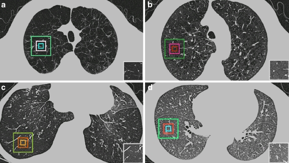
The visual characteristics for each of the four classes of images are illustrated in Figure 1 Panlobular or centrilobular emphysema produces small focal, approximately circular, areas of lung destruction that superficially resemble cysts (i.e., air-containing spaces sometimes with a thin definable wall), as shown in a case of severe centrilobular emphysema in Figure 1a. The conspicuity of the pattern is dependent on the severity of the disease. For a mild case, as shown in Figure 1b, the characteristic texture appearance is visible but less obvious. The air trapping and underperfusion caused by bronchiolitis obliterans results in homogeneously hypoattenuated lung, as shown in Figure 1c. For comparison, Figure 1-D shows the CT appearance of normal lung parenchyma.

Fig 1.

Axial thin-section CT scans of the chest (window level, −800 HU; width, 1,000 HU). On each image, the rectangles highlight three regions of interest (ROIs) with 16 × 16, 32 × 32, and 64 × 64 sizes that are typical of a particular condition. a Panlobular or severe centrilobular emphysema (PLE), b Mild centrilobular emphysema (CLE), c Bronchiolitis obliterans (BO), d normal lung parenchyma (NL). A typical normal lung region was selected in (d).

For each image, two thoracic radiologists with 10 years experience selected three sizes of concentric rectangular ROI (16 × 16, 32 × 32, and 64 × 64 pixels), which represent a typical area of lung parenchyma of each of three diseases or normal lung tissue with agreement. In this study, this classification was regarded as a gold standard. Areas between −400 and −1,024 HU were segmented for clipping major pulmonary vessels.

Feature Definition

From each ROI, texture and shape features were derived in the form of an N-dimensional vector v. The vector v contained the values of 13 texture features and 11 shape features chosen to describe the ROI characteristics. All features are listed in Table 1.

Table 1.

Summary of 13 Textural Features and 11 Shape Features that Represent Each ROI

Class	Descriptor	Dimension
Texture features	Histogram	Density mean
		Density SD
		Skewness
		Kurtosis
	Gradient	Gradient mean
		Gradient SD
	Run-length matrix	Short primitive emphasis
		Lung primitive emphasis
	Co-occurrence matrix	Angular second moment
		Contrast
		Correlation
		Inverse difference moment
		Entropy
Shape features	Top-hat transform	White top-hat mean
		White top-hat SD
		Black top-hat mean
		Black top-hat S.D.
	Cluster	Number of cluster
		Area mean
		Area SD
		Circularity mean
		Circularity SD
		Aspect ratio mean
		Aspect ratio SD

Texture Features

As the typical texture features, histogram features (mean, SD, skewness, and kurtosis), gradient features (mean and S.D.), run length encoding (short and long primitive emphasis), and co-occurrence matrix (angular second moment, contrast, correlation, entropy, and inverse difference momentum) were employed.⁴

The features that described the spatial dependence of gray-scale distributions were derived from the set of co-occurrence matrices. Since histogram and co-occurrence matrix-based features do not represent the length of the gray level primitives, acquisition-length parameters were also computed at each ROI to provide another set of features to be included in the feature vector v.

Shape Features

Textural features do not capture effectively the characteristics of a specific type of shape in the CT image. In the case of obstructive lung diseases, LAA, segmented by thresholding below −950 HU, is regarded as representing the disease. To reduce the noise of HRCT reconstructed by B70f kernel, median filter of 3 × 3 kernel size was applied three times. By thresholding −950 HU, all LAA objects were recognized and labeled. For the shape descriptors, the size of LAA (mean and SD), number of emphysema clusters, circularity, (1) circularity SD, aspect ratio, (2) and aspect ratio SD of the objects at each ROI were included. The circularity and aspect ratio of cluster were computed as follows⁸:

1

2

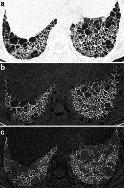
In addition, mean and SD of objects of subtraction image from white and black top-hat transformation result to original image were used. The white and black top-hat transform, which detects the top/bottom region of image density distribution, was employed. The image was rescaled using −748 HU upper threshold and −1,024 HU lower threshold. White top-hat transform detects the top white region with the given size of structure element by gray scale morphological operators of erosion and dilatation⁹. The gray scale erosion and dilatation operator cut off the top region. The subtraction of the resulting image from the original image finally produces the white top-hat transformed image. The mean and SD of segmented objects were calculated from the top-hat transformed images at each ROI. Black top-hat transform uses the inversion of the image and applies the procedure which is the same to the white top-hat transform. Figure 2 shows the original image and white and block top-hat transformed images.

Fig 2.

Original HRCT image and top-hat transformed HRCT images. a original HRCT image, b white top-hat transformed image, c black top-hat transformed image.

In summary, each ROI was characterized by the 24-dimensional vector v, which contained the feature values (Table 1).

Machine Learning Method

As a subfield of artificial intelligence, machine learning is concerned with the design and development of algorithms and techniques that allow computers to learn. In general, to avoid overestimating the classification accuracy, the gold standard data is split into exclusive training and testing data sets. In this study, the machine learning method trained the training data set of the gold standard and generated its own model. By using this model, the classifier classified the testing data set and determined its own accuracy based on the gold standard.

Feature Selection Method

It is useful to identify the subset of input variables that contribute most in the classification. The elimination of irrelevant input features that introduce noise often improves classification performance. Besides better overall sensitivity, a smaller number of features reduces the time spent, especially for the real-time classification. Exhaustive search over all possible combinations of input variables to identify the optimal subset is known as NP-complete problem.¹⁰ In the study, five different types of feature selection methods which rank the variables and identify the near-optimal subset were tested and compared based on the classification performance and clinical applicability: sequential forward selection (SFS), sequential backward selection (SBS), plus l-take away r (PTA(l,r)), sequential floating forward selection (SFFS), sequential floating backward selection (SFBS).¹¹ For example, in SFS, it starts with all input variables and sequentially deletes the next variable that mostly decreases the classification performance at that step. This greedy feature selection method may not find the optimal feature set, but nonetheless, their time complexity is only linear in the number of features compared with the exponential growth for the exhaustive search.

Experimental Settings

For the optimization of classifier, various experiments have been conducted. At first, various optimal binning sizes were evaluated. For validation of usefulness of new shape analysis, the only 13 texture features and the 11 shape features with the texture features were separately employed to build a classifier. For validation of the usefulness of the feature selection method, the full and the refined feature sets from the full feature set obtained by the various feature selection methods was also evaluated and compared. To evaluate which classifier shows better performance on this problem, Bayesian classifier and support vector machine (SVM) were implemented and compared.

Optimal Binning

The bin size could influence on the performance of classifier.¹² To find optimal binning, variable linear binning sizes (Q, bin size: 16, 32, 64, 128, 144, 196, and 256) of run length encoding and co-occurrence matrix were tested. The overall accuracy of Bayesian classifier was used as a metric to find an optimal combination of all ROI size, and binning sizes for run length encoding and co-occurrence matrix. Every following experimental test was performed with experimental optimal conditions, except the ROI size. In the case of ROI size, in general, a smaller ROI size is preferred, because the smaller ROI is regarded as representing better locality of lung parenchyma and showing better classification results, overlaid on lung HRCT images.

Cross-Validation

To check cross-validity of input data, a fivefold cross-validation scheme to evaluate the classifiers was employed. The five-folding cross-validation was performed as follows: the data set of each class was divided uniformly and randomly into five exclusive stratified subsets. Four subsets from the all subsets in turn, which constructed each fold at a time, were chosen. In this way, five folds, of which distributions are similar to original data, were obtained. Each fold was in turn held aside as the test set, when the other exclusive four subsets were used to train the classifiers. The average of the five folds cross validation results was employed for overall result of each classification method. To facilitate training, it is necessary to normalize the distribution of features to have zero mean and unit variance. The distribution of feature which is normal for the Bayesian classifier was assumed.

Machine Classifiers Implementation and Setting

The Bayesian classifier was implemented using MATLAB (The MathWorks, Natick, MA, USA).^13–15 To validate the performance, the Bayesian classifier was tested twenty times repeatedly, since results may have a variance with randomly chosen data set. In the SVM, the classifier using the MATLAB OSUSVM Toolbox was employed¹⁶. Note that the SVM is associated with a few model parameters that need to be fine-tuned during training for best performance^17–23. The testing on which type of kernel functions (i.e., radial basis function versus polynomial) and what its associated parameters (i.e., the kernel width σ for radial basis function and the order p for the polynomial) are better was performed; in addition, it also needs to determine the regularization parameter C. The kernel type used in this study is the radial basis function. Various gamma values and costs were tested to optimize the performance of SVM for each ROI size in the range of 0.01~10 and 10~1,000 by a unit of 0.01 and 10, respectively. All user-chosen parameters were listed in Table 2.

Table 2.

User Chosen Parameters for SVM

Feature	ROI	Gamma	Cost
Texture feature set	16	0.09	70
	32	0.06	70
	64	0.06	100
Texture + shape feature set	16	0.03	60
	32	0.03	40
	64	0.04	40
Refined feature set	16	0.12	50
	32	0.12	70
	64	0.15	20

Statistical Analysis

For every case, training and testing were conducted 20 times, and each case was performed five times for fivefold cross-validation. For comparison of time complexity of classifiers, testing time was measured in a unit of an experiment which consists of testing 256 ROIs with 100 repetitions. All the testing results were statistically compared (t test; significant alpha, 0.01) except for normality testing (significant alpha, 0.05). All the statistical analysis was performed in this study by Statistica™ 7.0 (StatSoft, Tulsa, OK, USA).

Experiment Results

ROI and Optimal Binning Size

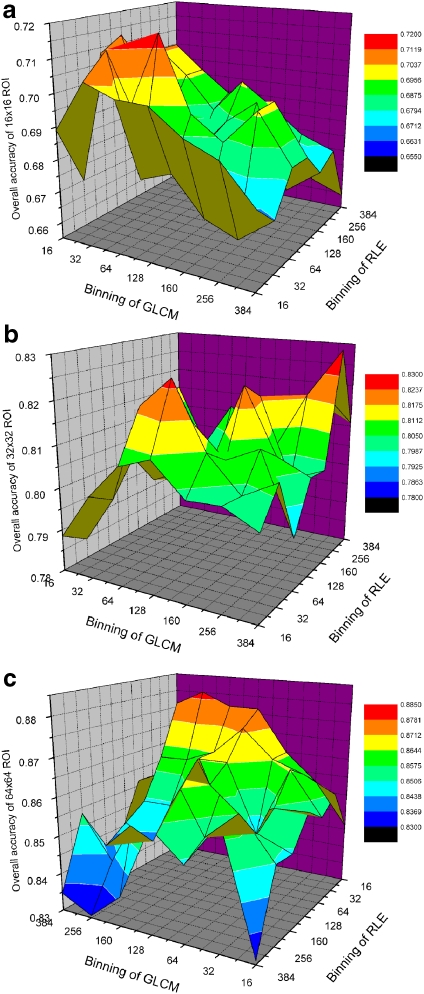
Figure 3 shows the experimental result of overall accuracy of various binning with each ROI size. The overall accuracy was improved in proportion to increase of ROI, regardless of classifier and feature set (t test, p < 0.01). This seems so natural since large ROI may contain more information.

Fig 3.

Experimental result of overall accuracy of various binning at each ROI size. a in case of 16 × 16 ROI size, b in case of 32 × 32 ROI size, c in case of 64 × 64 ROI size.

Table 3 shows the overall accuracy of every binning size (Q) at 64 × 64 ROI size. The tested optimal parameters resulted in 64 × 64 pixels of the ROI size, 16 of run length encoding and 256 of co-occurrence matrix, respectively (t test, p < 0.01).

Table 3.

Overall Accuracy of Every Binning Size (Q) of 64 × 64 ROI Size

RLE\GLCM	16	32	64	128	160	256	384
16	0.8462	0.8576	0.8649	0.8765	0.8765	0.8801	0.8760
32	0.8574	0.8617	0.8648	0.8723	0.8647	0.8615	0.8611
64	0.8535	0.8649	0.8459	0.8646	0.8645	0.8498	0.8497
128	0.8574	0.8570	0.8535	0.8606	0.8797	0.8417	0.8457
160	0.8497	0.8531	0.8645	0.8723	0.8643	0.8494	0.8417
256	0.8503	0.8608	0.8534	0.8684	0.8647	0.8421	0.8534
384	0.8310	0.8611	0.8496	0.8570	0.8377	0.8306	0.8346

Feature Selection Methods

These five feature selection methods were performed. Based on the experimental results, characteristics of each feature selection method were evaluated in terms of classification accuracy, robustness, and number of iteration (Table 4).

Table 4.

Accuracy, Number of Iteration at Maximum Accuracy, and Total Iteration Number at each Feature Selection Method and ROI Size

Parameter			SFS	SBS	PTA(3,2)	SFFS	SFBS
ROI	16	Accuracy	85.0	83.2	84.6
		Iteration num at Max	5	51	17
		Total iteration	55	54	265
	32	Accuracy	80.5		84.0
		Iteration num at Max	5		30
		Total iteration	55		265
	64	Accuracy	81.7	84.9	85.7	85.8	82.9
		Iteration num at Max	21	46	39	36	123
		Total iteration	55	54	265	113	150

SFS Sequential forward selection, SBS sequential backward selection, PTA(l,r) plus l-take away r, SFFS sequential floating forward selection, SFBS sequential floating backward selection

All study was performed using the SVM classifier.

There were no significant accuracy differences among the algorithms, but there are wide differences of classifier accuracy pattern and number of iteration at maximum accuracy. The accuracy at the SFS method shows fast increase and fast decrease of classifier accuracy. PTA shows slower increase and mild decease. SFFS shows fast increase and a plateau.

Classification Using the Texture Features

Classification experiment with 13 texture features was performed at first to get a base classification performance for evaluation of the effect of adding shape features to the classifier. Testing time, overall sensitivity, SD of overall sensitivity, sensitivity, and specificity for each of the four classes are given in Table 5. The best performance was achieved by the SVM with 64 × 64 pixels of ROI. Two classifiers showed similar results; ROI size had a significant effect on overall sensitivity. As ROI increases, the overall sensitivity becomes higher (t test, p < 0.01). Among four classes, the CLE was most hard to classify correctly in every ROI size, while PLE was easy to classify comparatively. In the term of testing time, SVM was quite fast (took less than 0.4 s to test all sample 20 times). The Bayesian, however, consumed more than 7.0 s. Testing time was measured in a unit of an experiment which consists of testing 256 ROIs with 100 repetitions.

Table 5.

Overall Sensitivity, Class-Specific Sensitivity, and Specificity Based on the Texture Features

Classifier	ROI	Testing Time(s)	Overall Sensitivity (%)	S.D. (%)	Sensitivity (%)				Specificity (%)
					PLE	CLE	BO	NL	PLE	CLE	BO	NL
Bayesian	16	7.04	65.9	1.5	88.3	39.3	56.1	80.8	96.9	85.2	92.1	80.3
	32	7.01	76.1	1.2	93.7	69.7	62.1	82.0	97.9	87.6	92.9	90.2
	64	7.23	85.3	0.9	97.5	79.4	78.1	86.6	98.7	92.5	94.3	94.7
SVM	16	0.30	66.3	1.4	86.6	46.8	58.9	73.7	94.7	83.3	91.9	85.4
	32	0.33	77.3	1.3	96.1	70.4	65.4	79.0	97.5	88.7	92.2	91.9
	64	0.20	85.8	1.2	95.9	78.5	76.9	92.6	98.0	91.6	95.6	96.0

PLE Panlobular or severe centrilobular emphysema, CLE mild centrilobular emphysema, BO bronchiolitis obliterans, NL normal lung parenchyma.

Classification Using the Texture and Shape Features

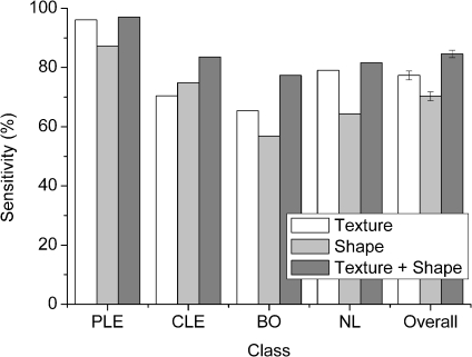
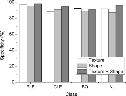
Eleven shape features in existing 13 texture features were added to the feature set, and classifiers ware tested. Testing time, overall sensitivity, SD of overall sensitivity, sensitivity, and specificity for each of the four classes are given in Table 6. In a comparison to the result using only texture feature, adding the shape features yielded better overall sensitivity regardless of ROI and classifier (t test, p < 0.01). The following have the same result as the texture feature experiment: the overall sensitivity was improved in proportion to the increase of ROI size in every classifier (t test, p < 0.01). Comparing the sensitivity of four classes, CLE had the worst sensitivity in every case, while PLE had the best one (t test, p < 0.01). The differences in class-specific sensitivity in the Bayesian classifier, however, are pretty larger than the SVM classifier. The class-specific sensitivity for each classifier is displayed in Figures 4 and 5. In the Bayesian classifier, testing time was increased up to at least 11.2 s, while it was not increased in the SVM classifier compared to using only texture feature.

Table 6.

Overall Sensitivity, Class-Specific Sensitivity and Specificity Based on the Full Feature Set

Classifier	ROI	Testing time(s)	Overall sensitivity (%)	SD (%)	Sensitivity (%)				Specificity (%)
					PLE	CLE	BO	NL	PLE	CLE	BO	NL
Bayesian	16	11.20	73.2	1.7	91.3	76.7	64.8	61.4	99.1	84.7	86.4	93.8
	32	11.82	82.2	1.2	97.0	87.3	73.9	71.9	99.1	92.9	89.4	94.7
	64	11.57	89.4	1.0	99.3	92.9	83.9	82.4	98.8	95.8	93.1	98.2
SVM	16	0.33	75.4	1.6	92.4	74.4	61.2	75.3	96.7	90.2	89.8	91.0
	32	0.28	84.8	1.3	96.7	83.1	78.1	82.3	98.2	94.6	91.0	96.2
	64	0.32	92.2	1.1	99.0	92.8	83.9	93.8	98.6	96.5	97.4	97.3

PLE Panlobular or severe centrilobular emphysema, CLE mild centrilobular emphysema, BO bronchiolitis obliterans, NL normal lung parenchyma

Fig 4.

Sensitivity over feature set (SVM classifier, 32 × 32 ROI size).

Fig 5.

Specificity over feature set (SVM classifier, 32 × 32 ROI size).

Classification Using the Refined Features by Feature Selection Method

Finally, an experiment using refined feature set from full feature set by the forward elimination feature selection method was performed. The number of refined features and eliminated features are listed in Table 7. Many shape features survived after the feature selection. In comparison to the experiment using all texture and shape feature, the experiment using refined feature set yielded better overall sensitivity regardless of ROI and the type of classifiers, especially in the SVM classifier (t test, p < 0.01; Table 8). The SVM classifier yielded the best overall sensitivity 93.5% with 64 × 64 pixels of ROI size (t test, p < 0.01).

Table 7.

The Number of Refined Feature and Added Features

Classifier	ROI	Number of refined feature	Added featuresa (shape features)
Bayesian	16	13 (6)	7, 11, 21, 23, 2, 1, 12, 18, 22, 4, 8, 16, 20 (16, 18, 20, 21, 22, 23)
	32	19 (8)	7, 11, 3, 17, 21, 16, 23, 4, 1, 18, 14, 20, 22, 9, 6, 5, 13, 2, 24 (13, 16, 17, 18, 20, 21, 22, 24)
	64	16 (8)	7, 11, 21, 18, 15, 14, 16, 1, 3, 22, 23, 4, 13, 6, 12, 9 (13, 14, 15, 16, 18, 21, 22, 23)
SVM	16	14 (8)	7, 13, 20, 24, 5, 2, 19, 16, 1, 6, 23, 21, 11, 17 (13, 16, 17, 19, 20, 21, 23, 24)
	32	17 (9)	8, 9, 7, 11, 21, 15, 23, 16, 18, 5, 22, 17, 1, 14, 3, 24, 2 (14, 15, 16, 17, 18, 21, 22, 23, 24)
	64	15 (5)	8, 12, 4, 9, 8, 11, 21, 20, 7, 18, 22, 5, 1, 16, 3 (16, 18, 20, 21, 22)

^aFeatures were listed in order of selected features by the forward feature selection method

Table 8.

Overall Sensitivity, Class-Specific Sensitivity, and Specificity Basis on the Refined Feature Set

Classifier	ROI	Testing Time(s)	Overall Sensitivity (%)	SD (%)	Sensitivity (%)				Specificity (%)
					PLE	CLE	BO	NL	PLE	CLE	BO	NL
Bayesian	16	6.39	76.9	1.4	93.7	70.2	59.1	85.2	98.4	90.4	92.4	87.9
	32	8.70	83.8	1.2	97.0	81.9	71.7	85.3	99.3	93.6	91.6	93.8
	64	7.95	90.3	0.8	100.0	89.8	83.2	88.7	98.,8	97.2	94.9	96.0
SVM	16	0.35	77.9	1.4	95.5	73.4	64.5	78.8	97.6	91.8	92.6	88.8
	32	0.18	85.9	1.0	98.3	82.2	78.8	84.7	98.6	95.5	91.4	95.9
	64	0.17	93.5	1.0	99.8	92.3	88.3	93.8	98.9	96.4	98.2	97.9

PLE Panlobular or severe centrilobular emphysema, CLE mild centrilobular emphysema, BO bronchiolitis obliterans, NL normal lung parenchyma

Contribution of Shape Features

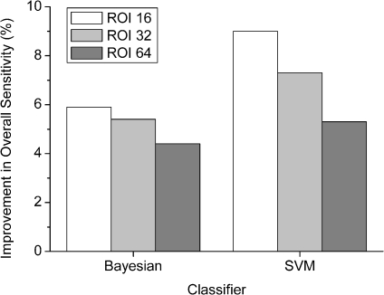
In the experiments, the performances of machine classifiers with the three different feature sets were tested to evaluate the usefulness of shape features for differentiation of obstructive lung diseases. In a comparison to employing only the texture feature set, the full feature set yielded higher overall sensitivity 7.3%, 6.1%, 4.1% in the Bayesian classifier and 9.1%, 7.5%, 6.4% in the SVM classifier in the order of ROI size 16 × 16, 32 × 32, 64 × 64 pixels, respectively (t test, p < 0.01). Improvements in overall sensitivity of each ROI size are shown in Figure 6. According to these experimental results, the composition of shape and texture features is useful to improve classification accuracy of obstructive lung diseases in both classifiers.

Fig 6.

Improvement of overall sensitivity with adding shape features to texture features based on the ROI size.

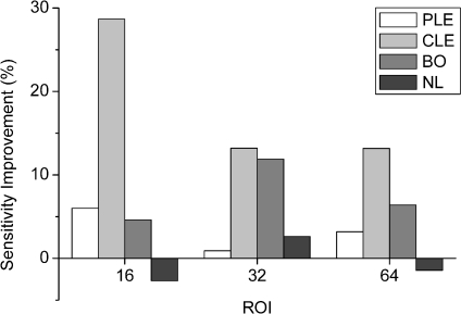
The improvement was largely due to the improvement of sensitivity of CLE and BO. For example, employing shape features yielded 20.3% for CLE and 18.7% for BO higher class-specific sensitivity than those of employing only texture features (SVM, 32 × 32 pixels of ROI). Improvements on class-specific sensitivity are displayed in Figure 7 for the SVM classifier.

Fig 7.

Improvement of class specific sensitivity with adding shape features to texture features based on the ROI size in the SVM classifier.

Discussion

Effect of ROI Size

Employing shape features improved overall sensitivity regardless of ROI size and classifier, and the improvements were larger in the smaller ROI size. The improvement of overall sensitivity at each ROI size is displayed in Figure 8.

Fig 8.

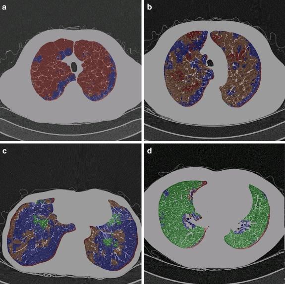
Application of the classifier to differentiation of lung parenchyma. At every pixel, the semi-transparent color was coded by the classification result. (a) CT scan obtained in a patient with PLE. Most of the parenchyma was labeled as severe emphysema. (b) CT scan obtained in a patient with signs of CLE. Most of the classified samples were labeled as CLE. Some areas of the lung with homogeneously decreased attenuation and large air cysts were classified as BO or PLE. (c) CT scan in a patient with BO. Most of the parenchyma was labeled as BO, whereas some areas were classified as normal lung parenchyma. Areas of the lung with increased attenuation adjacent to areas of decreased attenuation allow the classifier to identify the texture of CLE in the vicinity of the major bronchi. (d) CT scan obtained in a healthy subject (window level, −850 HU; width, 400 HU) with automated classification. Samples classified confidently are labeled as normal. For color figures, please go to Springerlink to view the online version.

It is interesting that the shape analysis improved the overall sensitivity at smaller ROI. In clinical application, smaller ROI may be preferred because smaller ROI may represent local property better. Therefore, for the whole lung classification, the shape analysis is regarded as more clinically useful in the terms of ROI size as well as overall sensitivity.

Feature Selection Methods

In Figure 3, SFFS shows fast increase and lasting plateau of accuracy performance, which means that the robustness of SFFS is regarded as better than other methods. In addition, there is a possibility to apply early termination with high accuracy with relatively small number of iteration.

Considering the number of iteration, SBS needs much more iterations than SFS (Table 4). This means there will be a critical problem, if there are many features.

Gold Standard Acquisition

The reliability of subjective visual assessment for this classification is open to question. Other methods, however, such as pulmonary function tests, do not reliably distinguish between the various pathologic causes of obstructive lung diseases. Biopsy is not performed routinely in patients with obstructive pulmonary disease, either because patients have such severe disease that surgery is precluded or because they have mild disease that does not warrant an invasive procedure. Furthermore, there are regional differences in the predominant disease; in patients with emphysema, areas of mild and severe disease may coexist in different parts of the lungs. Despite its limitations, CT evaluation by two experienced radiologists is a reasonable standard of reference. All of tested classifiers based on the texture and shape feature set achieved high sensitivity and specificity. Irrespective of the diagnostic reliability of subjective assessment, both classifiers with the texture and shape feature set classify ROI in a way that is consistent with that of the experienced observer who provided the training data; nevertheless, the ability of the classifier to successfully match image chosen by one observer falls short of fully competent diagnostic performance.

Contingency Matrix

The largest number of cases of misclassification resulted from confusion between cases of NL and BO in this study. The confusion between cases of CLE and BO also occurred frequently. This is not surprising, given the similar visual appearances at CT for these two conditions. On the other hand, misclassification of the PLE rarely occurs in all classifiers. This is reasonable because the image of PLE has a prominent characteristic in comparison to other diseases. An example contingency matrix is given in Table 9. The bold numbers in Table 9 represent major misclassifications between the BO and CLE. Nevertheless those confusions between diseases, the general discriminating values of two classifier bases on the texture and shape feature set were demonstrated, with higher overall sensitivity and specificity than the classifier basis on the only texture feature.

Table 9.

An Example of Contingency Matrix with SVM Classifier, Texture, and Shape Feature Set, and 32 × 32 ROI Size

Parameter		Predicted
		PLE	CLE	BO	NL
Actual	PLE	96.7	1.4	2	0
	CLE	1.5	83.1	11.8	3.5
	BO	3.7	10.4	78.1	7.8
	NL	0	4.4	13.3	82.3

PLE Panlobular or severe centrilobular emphysema, CLE mild centrilobular emphysema, BO bronchiolitis obliterans, NL normal lung parenchyma.

Normal Distribution Assumption

The assumption that the features in each class are distributed normally can also be questioned. In the normality test, 1~3 of the distribution of features in all ROI size was not normal. The significance level was 0.05, and the rejection region was χ² > 5.991. It could affect the performance of the naïve Bayesian and Bayesian classifier which relies on the assumption regarding the underlying class-specific probability distribution. However, it has been demonstrated that Bayesian classifiers with such a probabilistic model were robust, even when the assumption on class-specific probabilities being normally distributed was considerably violated²⁴. Furthermore, the number of features with a probability distribution that is not normal was small. Hence, this assumption is reasonable and could not affect the performance of those two classifiers.

Training and Testing Time

Training time could be an issue if the classifier is required to be updated dynamically. In this case, the Bayesian and SVM classifiers would be appropriate. Since it is enough to update a classifier once weekly or monthly in the real world, training time is not so important. Testing, however, is conducted repeatedly on new samples. Hence, testing time is critical for clinical applications such as a color disease overlay program. For example, the system implemented in Figure 8 needs about 10,000 iterations of pixel-by-pixel testing to completely color mask a CT image. We therefore measured the time needed to test 265 samples. We found that the testing time of the SVM classifier did not exceed 0.02 s in any case, whereas the Bayesian method spent about 3.35 s. The SVM classifier would take less than 0.4 s to classify all samples, whereas the Bayesian classifiers would take about 2 s (Tables 6 and 8). The SVM methods are regarded as acceptable for clinical applications in terms of testing speed.

Conclusions

We have demonstrated that not only texture features, but also shape features are useful in constructing classifier of several diseases that cause decreased attenuation of the lung parenchyma. Adding shape features, the Bayesian and SVM classifier achieved higher overall sensitivity than those based on the only texture features in every ROI size. The overall accuracy was significantly improved in proportion to increase in ROI, regardless of classifier and feature set. In addition, the tested optimal parameters resulted in 64 × 64 pixels of the ROI size, 16 of run length encoding, and 256 of co-occurrence matrix, respectively. Based on these optimal parameters, the best overall sensitivity of 93.5% was achieved by the SVM classifier based on the optimized feature set. The shape features contribute more to the overall accuracy in the case of smaller ROI with the SVM classifier, which is good property on the clinical purpose.

The software used for this work is not available as open source, but the data set is available through Springer as supplemental data.

References

- 1.Copley SJ, Wells AU, Müller NL, Rubens MB, Hollings NP, Cleverley JR, Milne DG, Hansell DM. Thin-section CT in obstructive pulmonary disease: discriminatory value. Radiology. 2002;223(3):812–819. doi: 10.1148/radiol.2233010760. [DOI] [PubMed] [Google Scholar]
- 2.Chan K, Lee TW, Sample PA, Goldbaum MH, Weinreb RN, Sejnowski TJ. Comparison of machine learning and traditional classifiers in glaucoma diagnosis. IEEE Trans Biomed Eng. 2002;49(9):963–974. doi: 10.1109/TBME.2002.802012. [DOI] [PubMed] [Google Scholar]
- 3.Wei L, Yang Y, Nishikawa RM, Jiang Y. A study on several machine-learning methods for classification of malignant and benign clustered microcalcifications. IEEE Trans Med Imaging. 2005;24(3):371–380. doi: 10.1109/TMI.2004.842457. [DOI] [PubMed] [Google Scholar]
- 4.Chabat F, Yang GZ, Hansell DM. Obstructive lung diseases: texture classification for differentiation at CT. Radiology. 2003;228(3):871–877. doi: 10.1148/radiol.2283020505. [DOI] [PubMed] [Google Scholar]
- 5.Xu Y, Beek EJ, Hwanjo Y, Guo J, McLennan G, Hoffman EA. Computer-aided classification of interstitial lung diseases Via MDCT: 3D Adaptive Multiple Feature Method (3D AMFM) Acad Radiol. 2006;13(8):969–978. doi: 10.1016/j.acra.2006.04.017. [DOI] [PubMed] [Google Scholar]
- 6.Rangayyan RM, Mudigonda NR, Desautels JE. Boundary modeling and shape analysis methods for classification of mammographic masses. Med Biol Eng Comput. 2000;38:487–496. doi: 10.1007/BF02345742. [DOI] [PubMed] [Google Scholar]
- 7.Yamagishi M, Koba H, Nakagawa A, Honma A, Yokokawa K, Saitoh T, Harada H, Watanabe H, Mori Y, Katoh S, et al. Qualitative assessment of centrilobular emphysema using computed tomography. Nippon Igaku Hoshasen Gakkai Zasshi. 1991;51(3):203–212. [PubMed] [Google Scholar]
- 8.Iwano S, Nakamura T, Kamioka Y, Ishigaki T. Computer-aided diagnosis: a shape classification of pulmonary nodules imaged by high-resolution CT. Comput Med Imaging Graph. 2005;29(7):565–570. doi: 10.1016/j.compmedimag.2005.04.009. [DOI] [PubMed] [Google Scholar]
- 9.Gonzalez RC, Woods RE. Digital Image Processing. 2. New Jersey: Prentice Hall; 2002. pp. 532–534. [Google Scholar]
- 10.Amaldi E, Kann V. On the approximation of minimizing non zero variables or unsatisfied relations in linear systems. Theor Comput Sci. 1998;209:237–260. doi: 10.1016/S0304-3975(97)00115-1. [DOI] [Google Scholar]
- 11.Kittler J: Feature set search algorithms. Pattern recognition and signal processing. Sijtho and Noordho 41–60, 1978
- 12.Handrick S, Naimipour B, Furst JD, Raicu DS. Binning strategies evaluation for tissue classification in computed tomography images. Proc SPIE Med Imaging. 2006;6144:1476–1486. [Google Scholar]
- 13.Vapnik VN. The Nature of Statistical Learning Theory. New York: Springer-Verlag; 2006. [Google Scholar]
- 14.Friedman N, Geiger D, Goldszmidt M. Bayesian network classifiers. Mach Learn. 1997;29:131–163. doi: 10.1023/A:1007465528199. [DOI] [Google Scholar]
- 15.Mitchell T. Machine Learning. New York: McGraw-Hill; 1997. [Google Scholar]
- 16.Joachims T, Schölkopf B, Burges C, Smola A. Making large-scale SVM learning practical. Advances in Kernel methods - support vector learning. Cambridge, MA: MIT-Press; 1999. [Google Scholar]
- 17.Boser BE, Guyon IM, Vapnik VN. A training algorithm for optimal margin classifiers. Proc Fifth Annu Workshop Comput Learning Theor. 1992;5:144–152. doi: 10.1145/130385.130401. [DOI] [Google Scholar]
- 18.Burges CJC. A tutorial on support vector machines for pattern recognition. Data Mining Knowledge Discovery. 1998;2(2):121–167. doi: 10.1023/A:1009715923555. [DOI] [Google Scholar]
- 19.Dumais ST. Using SVMs for text categorization. IEEE Intell Syst. 1998;13(4):21–23. [Google Scholar]
- 20.Burges CJC, Schölkopf B. Improving the accuracy and speed of support vector learning machine. Cambridge, MA: MIT Press; 1997. [Google Scholar]
- 21.Furey TS, Cristianini N, Duffy N, Bednarski DW, Schummer M, Haussler D. Support vector machine classification and validation of cancer tissue samples using microarray expression data. Bioinformatics. 2000;16:906–914. doi: 10.1093/bioinformatics/16.10.906. [DOI] [PubMed] [Google Scholar]
- 22.Ding CHQ, Dubchak I. Multi-class protein fold recognition using support vector machines and neural networks. Bioinformatics. 2001;16:349–358. doi: 10.1093/bioinformatics/17.4.349. [DOI] [PubMed] [Google Scholar]
- 23.Zien A, Rätsch G, Mika S, Schölkopf B, Lengauer T, Müller KR. Engineering support vector machine kernels that recognize translation initiation sites. Bioinformatics. 2000;16:799–807. doi: 10.1093/bioinformatics/16.9.799. [DOI] [PubMed] [Google Scholar]
- 24.Schurmann J. Pattern classification: a unified view of statistical and neural approaches. New York: Wiley, NY; 1996. [Google Scholar]