Shape-Adaptive DCT for Denoising of 3D Scalar and Tensor Valued Images

Abstract

During the last ten years or so, diffusion tensor imaging has been used in both research and clinical medical applications. To construct the diffusion tensor images, a large set of direction sensitive magnetic resonance image (MRI) acquisitions are required. These acquisitions in general have a lower signal-to-noise ratio than conventional MRI acquisitions. In this paper, we discuss computationally effective algorithms for noise removal for diffusion tensor magnetic resonance imaging (DTI) using the framework of 3-dimensional shape-adaptive discrete cosine transform. We use local polynomial approximations for the selection of homogeneous regions in the DTI data. These regions are transformed to the frequency domain by a modified discrete cosine transform. In the frequency domain, the noise is removed by thresholding. We perform numerical experiments on 3D synthetical MRI and DTI data and real 3D DTI brain data from a healthy volunteer. The experiments indicate good performance compared to current state-of-the-art methods. The proposed method is well suited for parallelization and could thus dramatically improve the computation speed of denoising schemes for large scale 3D MRI and DTI.

INTRODUCTION

Diffusion Tensor Magnetic Resonance Imaging (DTI) is an important magnetic resonance imaging protocol used in both research and in clinical applications. The DTI modality has the advantage that highly structured tissue, for example the nerve fibers in the human brain, can be studied noninvasively.^1,2 From a series (typically 6–50) of direction-sensitive MR acquisitions a 3×3 diffusion tensor can be estimated for each voxel of the imaging domain.^3–6 From these voxel-wise diffusion tensors, a number of interesting clinical quantities can be estimated and used to investigate or differentiate between normal and abnormal tissue, e.g., in Multiple Sclerosis or Schizophrenia research.^7–9

However, it is a well-known fact that the MRI signal from the scanner contains measurement noise, which degrades the quality of the images. In the following, we model the MRI true signal S^noisy as a composition of clean (or “true”) signal and additive normally distributed noise, for example.

1

Although we cannot in general assume that the noise is normally distributed with zero mean and variance σ², we may approximate the noise by such a distribution. The signal-to-noise-ratio (SNR) in DTI is low compared to standard MRI. This makes it important to construct good models and methods for noise removal for diffusion tensor data. Because of the huge amount of data, the methods should ideally be efficient with regards to computational time.

Several successful methods for denoising of diffusion tensor MRI have been proposed.^10–15 A large class of existing state-of-the-art methods are based on partial differential equations. The nature of these methods typically makes them computationally heavy. These methods are iterative methods, and often many computationally heavy iterations must be performed before convergence is reached. This is in particular true when gradient methods are used in the solution process. In this paper, we introduce an alternative method for regularization of matrix-valued images, based on application of the shape-adaptive discrete cosine transform (SA-DCT).^16–19 This is a direct method, i.e., only one “iteration” is needed in the solution process. Moreover, the method can be parallelized in a straightforward manner since the computations for each voxel can be performed without any knowledge of the computations performed in any of the other voxels. In the last section of this paper, we make a quantitative and visual comparison of the method proposed in this paper with a recently introduced Partial Differential Equations (PDE) method for regularization of tensor valued images.¹¹ Interestingly, we observe that the proposed transform-based method gives results, which are very similar to the results from the completely different PDE-based method. Although the SA-DCT methodology may not be superior to other methods, it is an interesting alternative methodology for denoising of tensor-valued images.

BACKGROUND

Diffusion Tensor Imaging

Tensor-valued data occur in many branches of mathematical sciences; see, e.g., Weickert and Hagen²⁰. In this paper, the tensor-valued data comes from diffusion tensor MRI of the human brain. From a set of K direction sensitive magnetic resonance images a symmetric positive definite tensor is constructed in each voxel of the image domain. This matrix yields structural information of the tissue in each voxel.

The relationship between each direction weighted measurement and the diffusion tensor D is given by the Stejskal–Tanner equation ^21,22

2

where b is a positive scalar given by the measuring pulse sequence, and is one of the predefined selected directions for which measurement S_k is acquired. From K direction weighted measurements we obtain K equations that we use for estimating the six unknowns of the diffusion tensor D. This can be done, for example, by a linear least-squares method, or other more adaptive methods.⁵ We note that as the transformation (Eq. 2) is nonlinear, we do not know the distribution of the noise in each element of the tensor D. Hahn et al.²³ have studied how noise propagates through the estimation process.

In structured tissue such as in the heart muscle or in the white matter of the brain, the self-diffusion of water is highly anisotropic. In gray matter and in cerebrospinal fluid, the self-diffusion of water is almost isotropic. Based on knowledge of the diffusion tensor D, a model of the myelinated nerve fiber pathways in the white matter can be constructed via fiber tracking algorithms.^1,2,24,25

The quality of the estimated diffusion tensor depends on several parameters. One particular parameter is the number of acquisitions or excitations (NEX) performed in each of the diffusion sensitizing directions. A high number of acquisitions in each direction gives a tensor estimate of good quality, provided the patient does not move during the acquisitions, whereas a small number of acquisitions give a shorter examination time for each patient. Therefore, we have a compromise between efficiency of the acquisitions and quality of the resulting images. In this paper, we investigate the possibility of post-processing the data from a small number of acquisitions, and still being able to construct tensor estimates of high quality. Thus, a practical research goal is to decrease the scanner time required for each patient.

Shape-Adaptive Discrete Cosine Transform

The 2-dimensional discrete cosine transform (DCT) is extensively used in image science. In its original formulation, it transforms a quadratic region in the spatial domain into the frequency domain. Being a harmonic transform, the DCT has a compactification property, i.e., good approximations of the image can be constructed by employing only a few of the coefficients in the frequency domain.^26,27 However, when the image domain of the transform contains sharp edges and only a few of the coefficients in the frequency domain are employed for the reconstruction to the spatial domain, various artifacts such as smearing of edges and Gibbs phenomena occur. To avoid these artifact, the region should be as homogeneous as possible. This is achieved by replacing the static regions from the standard DCT by regions Ω_x, which adapts to the information in the image around a point x. We choose these regions in such a way that the data can be well approximated by a smooth, slowly varying function. Such a function is well approximated by few coefficients from the frequency domain. The regions Ω_x should ideally not contain any discontinuities.

In a series of papers, Katkovnik, Foi, Egiazarian, Astola, and others describe shape adaptive DCT (SA-DCT) for denoising of 2D grayscale and color images.^16–19 The algorithm can be divided into three different stages: (1) construction of an adaptive neighborhood for each point in the domain, (2) transformation and thresholding of each neighborhood, and (3) estimation of the noise-free image. The adaptive neighborhoods are constructed by local polynomial approximations (LPA) in combination with the intersection of confidence intervals (ICI) rule. The transformation of each neighborhood to the frequency domain is done by a DCT algorithm, and hard thresholding is applied on the coefficients in the frequency domain. The inverse DCT algorithm is then applied. This results in a denoised region. Since each pixel x has its own region Ω_x, and in general these regions may overlap, we get an overcomplete basis. This overcomplete basis is used to construct the final image by weighting the basis elements in a proper way.

The state-of-the-art results obtained by the SA-DCT methods in 2D as well as their efficiency makes them attractive for denoising of 3D scalar valued images and 3D matrix valued images. In this paper, we extend the framework of SA-DCT to both 3D scalar valued and 3D matrix valued images.

METHODS

Shape-adaptive Discrete Cosine Transform

Let be a closed spatial domain of dimension N and denote the noisy data set, which is discretized on a uniform grid. In the rest of this, paper we restrict the attention to 2D and 3D data sets, i.e. . We refer to the resulting denoised data set as I⁻. Presently, we treat the standard deviation σ of the noise of I as an input parameter.

A main ingredient of the SA-DCT method is the adaptive neighborhood Ω_x surrounding each voxel x∈Ω. The idea is that this neighborhood should contain voxels that in some way are “similar”, or homogeneous. A neighboring point y∈Ω can either have an intensity I(y), which is close to the intensity I(x), or the intensities can differ substantially. In the case where I(y)≈I(x), we want to include the point y in the adaptive neighborhood of x, i.e., y∈Ω_x. To decide which voxels should belong to the adaptive neighborhood of a given point, we use local polynomial approximations (LPA) and the intersection of confidence intervals (ICI) rule.¹⁹

To construct the adaptive neighborhood, we consider a set of directions such that each component of θ_i is either −1, 0 or 1, but never all equal to zero. It follows that there must be 3^N −1 such directions in an N-dimensional data set. In 2D,¹⁸ there are eight such directions: the four cardinal and the four intermediate compass directions. In 3D, there are 26 unique directions following a similar pattern.

We span a star-shaped skeleton around each point x in the image domain by tracing the voxels along straight lines in the directions of θ_i. The length d_i corresponding to the straight line in the direction of θ_i in the skeleton is determined by the ICI algorithm. We close the skeleton such that it becomes a polygonal hull by joining neighboring endpoints of the vertices in the skeleton by line segments (in 2D) or triangles (in 3D). We denote the domain inside this closed polygonal hull by Ω_x. For each voxel in the image domain, such an adaptive neighborhood is constructed. The pseudocode for our SA-DCT denoising is given in Algorithm 1.

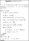
In the following section, we explain how we can use the LPA-ICI method to compute the length d_i of each branch in the star .

LPA-ICI

To span the region , we calculate the support of each branch in the star, i.e., number of voxels that should be included along each direction vector θ_i, i = 1,...,3^N − 1. The idea is that the voxels in should have intensity values that are close to the intensity value of the center voxel x. Variations in the included data should be caused by the noise level and small local variations, and not by edges in the image.

To achieve this, we filter each direction with LPA kernels of varying length (scale) h∈H={h₁,...,h_j}, where h₁<h₂<...<h_J. The generation of these filter kernels are described in Foi 2005.¹⁶ For each kernel g^(h) containing weights , where i = 1,..., h, we have the property that the center voxel x has the highest weight . In addition, the weights sum to 1 and decrease with the length of the filter.

We can consider this filtering as a convolution of the data with a filter kernel of varying length. When the kernel is applied to the voxels in direction θ_i, we get the filtered value

3

The standard deviation of the noise in μ^(h) is given through the relation

4

For each direction, we then get the confidence intervals

5

where Γ > 0 is a global parameter of the algorithm. A large Γ results in a large noise tolerance, and more voxels will be included in the regions, and vice versa.

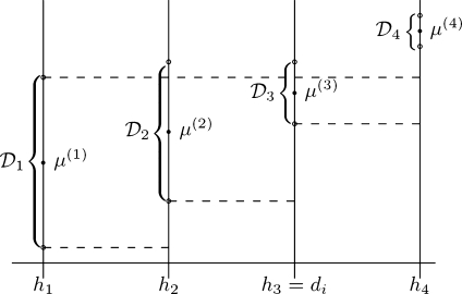
The ICI rule states that along the direction vector θ_i we should choose the largest distance d_i∈H where we have intersection of all the confidence intervals; see Figure 1. More precisely,

6

Fig 1.

An example of the LPA-ICI algorithm where H={h₁,...,h₄}. The area between the dashed lines shows the intersection of all previous confidence intervals. When the intersection is empty (here at h₄) the algorithm is terminated.

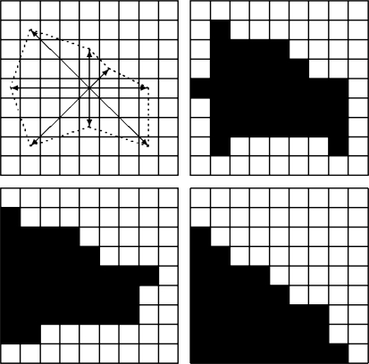
Having determined the length of each branch in the star- shaped domain , we define the neighborhood Ω_x as all voxels inside the polygonal hull closing with branches d_iθ_i, where i = 1,...,3^N − 1. By construction, the intensities in this region should not contain large changes caused by edges in the image. The noise in this region can now easily be removed by thresholding small coefficients in the frequency domain. We use the discrete cosine transform for this purpose as described in the next subsection. In the upper left panel of Figure 2, we have visualized an 2D example of the output of the LPA-ICI algorithm. The arrows centered around voxel x indicate each of the eight directions θ_i employed by the algorithm and the length of each arrow indicates the distance d_i. The set of all voxels covered by an arrow in the figure is and all voxels inside the dashed polygonal hull spanned by the arrows is Ω_x.

Fig 2.

Illustration of how coefficients are collected in one corner by Sikora’s algorithm (see the text for a description).

Note that since we only perform a LPA-ICI estimation on the voxels that coincide with the skeletonized domain , we do not have direct control over the intensity values in the set . It has been shown that for scalar images, this approach is a good compromise between efficiency and accuracy.¹⁷

Before the region Ω_x is denoised in the frequency domain, the mean of the region is estimated and subtracted from each intensity in Ω_x. This process is referred to as DC separation, and it has been shown to improve certain pathological issues associated with the shape-adaptive DCT described in the next section.¹⁷ After the DCT denoising is complete and the coefficients have been transformed back to the spatial domain, the precomputed mean is added to shift the mean of the intensities back to the same level as before the DCT. Although this shift of intensities is not entirely justified from the approximation standpoint (since the precomputed mean also will contain noise), it has been shown to visually provide superior results with few adverse effects.¹⁷

The DCT Algorithm

The discrete cosine transform (DCT) is used extensively in signal and image processing. The one-dimensional DCT of a signal {Z₀,...,Z_M−1} of length M is defined as

7

for k = 0,..., M − 1, where and . Note that this transform can be expressed as a matrix–vector product

8

When c_k is defined as above, then the A matrix is orthogonal. This implies that the inverse DCT can be expressed as

9

Two- and three-dimensional DCT are usually achieved by successively applying the one-dimensional DCT along the coordinate axes (i.e., separability). However, note that Ω_x will in general not be rectangular. Sikora has developed an algorithm for discrete cosine transform on nonrectangular domains.²⁶ In this paper, we employ this algorithm. However, we still use the orthogonal transform (Eq. 7) and not the one originally presented in Sikora 1995.²⁶

In the following, we let denote the quadratic (in 2D) or cubic (in 3D) null-extension of Ω_x. Null-extension in this context means a padding of the region with a particular value, “null”. This value will only be used as a “place-holder”, and not in any direct calculations. Accordingly, it is never considered a coefficient in the discussion below. The purpose of the null-extension is to extend the size of the region into a more manageable form, as later described.

Note that when examining Ω_x along the coordinate axes, it may be noncontiguous. One approach to alleviate this problem could be by zero-padding the region instead. However, this causes problems when applying the traditional DCT algorithm as many components of the DCT domain will be needed to represent these high jumps in intensities introduced by zero-padding. Sikora’s approach avoids this problem by first shifting all nonnull values of along the first coordinate axis so that they become consecutive in . A one-dimensional DCT, where the length of the signal M is equal to the number of nonnull values, is then applied to the shifted data. The same procedure is then applied to each dimension in turn, by first shifting the data and then applying the 1D DCT. When applying the inverse DCT, we need to invert these shifts, so a record of the rearrangements must be maintained.

In Figure 2 we display a 2D example of how the null-padded voxels are shifted to produce consecutive values. The upper right panel shows the null-padded region, where black is used to indicate voxel intensities (and later DCT coefficients) and white is used to show null values. The lower left panel shows the intensities shifted in the x direction towards the origin in the lower left corner. A 1D DCT is then applied to the nonnull elements of each row containing nonnull values; first to row 2 containing M = 1 intensities, then to row 3 containing M = 4 consecutive intensities, and so forth. The lower right panel shows the results after the row-wise DCT, shifted along the y axis. Again a 1D DCT is applied, this time to each nonnull element of each column. When the data is 3D, this procedure has to be repeated again in the z-direction. The final configuration is a set of shifted DCT coefficients in the origin corner of the cube.

Thresholding in the DCT Domain

Let denote the domain transformed from Ω_x using the DCT algorithm described in the previous section and let denote a given coefficient in . In addition, let denote the number of coefficients in the neighborhood . The cutoff threshold f is given as¹⁹

10

and the hard thresholded coefficients are given as

11

for all .

The thresholded region is then transformed and shifted back into the spatial domain by the inverse DCT giving in the spatial domain.

Estimation from Overcomplete Basis

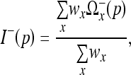
Notice that since we calculate a region Ω_x for every voxel in the image, we have extensive region overlap, i.e., we have an overcomplete basis. To reconstruct an image from this information, we weight the data together. We assign a weight to every region and use the information in overlapping regions to estimate the denoised image. It is a standard approach to use weights that are inversely proportional to the mean variance of the region. However, for adaptive regions this leads to oversmoothing.¹⁷ To compensate for this, we can divide the weights by the square of the size of the region.

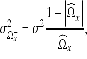
The mean variance of the region is given by

12

where is the number of nonzero coefficients in . This gives the following weights for the regions

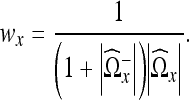13

The regions can now be weighted together, giving the final recovered estimate using the relation

14

for all p∈Ω and where the sum is taken over all voxels x such that contains p.

Generalization to DTI

In the previous section, we extended the SA-DCT methods from 2D to 3D images. This code can be used directly for denoising of 3D MRI images. In this section, we will show how the code also can be applied for matrix-valued DTI images.

In a previous work, two of the authors have investigated total variation (TV) regularization of tensor-valued data,¹¹ where the estimated tensor is regularized. To ensure positive definiteness of the regularized tensor, it is represented implicitly by Cholesky factorization as D=LL^T, where L is a lower triangular matrix. In the present work, we have adopted this approach when regularizing tensor-valued data by SA-DCT methods. Thus, we apply the 3D algorithm to each of the elements of L.

We are aware that there are other ways to apply the 3D code on matrix-valued DTI images, e.g., we could denoise directly on the S_i images. However, the advantage of the presented method is that we are able to guarantee positive eigenvalues. In addition, we have conducted numerical tests that indicate that the performance is similar for both methods.

EXPERIMENTAL RESULTS

In this section, we show qualitative numerical results achieved by the method proposed in this paper. We process both synthetically produced images and real diffusion tensor images of a healthy human volunteer.

3D Scalar-valued Data

We have in this paper generalized the SA-DCT methods from 2D to 3D images. In the first example, we want to show the difference between the 2D SA-DCT algorithm applied slice by slice in a 3D data set, referred to as quasi-3D, and application of our genuine 3D algorithm. We use 3D data from the BrainWeb, a database of freely available semirealistic simulated MR images.²⁸ The true data set has a range from 0 to 1 and a mean of 0.26. The added noise is normal distributed with zero mean and a variance of 0.07.

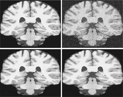
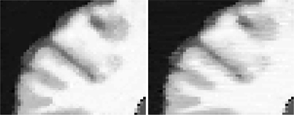
In Figure 3 we show a coronal slice of the image comparing the performance of the quasi-3D SA-DCT algorithm and the genuine 3D version. Line artifacts between neighboring slices can be observed, since the 2D algorithm ignores information in the z-direction. An additional problem with the 2D approach, dealing with isotropic voxels, is determining which axis to slice across. We have arbitrarily chosen the z-direction, but a choice of x or y would in this example yield different suboptimal results. As we observe from Figure 3, the result from the full 3D algorithm proposed in this paper yields results in which the noise reduction is performed in a consistent manner across all three dimensions. In Figure 4 we show a zoom-in of a small portion of the result from Figure 3.

Fig 3.

The difference between application of the 2D SA-DCT along coronal slices of a 3D image, and application of the genuine 3D SA-DCT algorithm. Upper left panel: the original true image. Upper right panel: the noisy image (zero mean, σ² = 0.07). Lower right panel: result after application of the quasi-3D algorithm along the z-direction. Lower left panel: result after application of the full 3D algorithm proposed in this paper. See also detail in Figure 4.

Fig 4.

Zoomed-in detail from Figure 3. Left panel: result after application of the genuine 3D algorithm. Right panel: result after application of the quasi-3D algorithm. Notice the slightly improved distinction between white matter, gray matter, and CSF, when the genuine 3D algorithm is applied.

We define the error as the Euclidean 2-norm of the difference between the noise-free image and the denoised image. The error between the noisy image and the noise-free image was 140.13. The image denoised using the quasi-3D algorithm gave 47.60, and using the full 3D algorithm reduced the error to 41.92.

3D Tensor-valued Synthetic Data

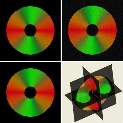
The main motivation behind this paper is denoising of tensor-valued images, in particular diffusion tensor MR images. First, we denoise a synthetic DTI data set where the object is a simulated torus. The DTI torus has been generated using the software Teem, written by Gordon Kindlmann.²⁹ For visualization of the color-coded fractional anisotropy (FA) images, derived from the estimated tensor images, we have used DtiStudio developed by Susumu Mori and coworkers.³⁰

Our DTI phantom consists of a doughnut-shaped object with cigar-shaped diffusion in the direction of the main circumference. The baseline image S₀ is constant equal to 1 and the six direction sensitive measurements S₁,...,S₆ have the range 0 to 0.80. We added normal distributed noise with zero mean and a variance of 0.01 to S₀ and variance of 0.04 to S₁,...,S₆. The six gradient directions g₁,...,g₆ used are given by the columns of the matrix

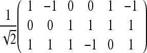The diffusion tensors computed from the clean DTI data is used as a reference and the denoised tensors are compared against this ground truth. We define the error as the sum of squared element-wise tensor differences

15

where D_ij(p) denotes the tensor element in position (i,j) at voxel p. The global error in the noisy data was found to be 95.86.

When first computing the diffusion tensors from the noisy DTI data and then apply the 3D SA-DCT algorithm to each of the six elements of the voxel-wise lower triangular L decomposition of the tensor, the global error was 18.03. The results of this denoising procedure are shown in Figure 5.

Fig 5.

Results from application of the proposed 3D SA-DCT algorithm to a synthetically produced diffusion tensor dataset where the object is a torus. Upper left panel: the true (noise-free) data. Upper right panel: the noisy data. Lower left panel: the denoised data. Lower right panel: 3D view of the torus. All figures are color-coded FA plots derived from the tensor.

3D Tensor-valued Real Brain Data

Finally, we tested SA-DCT denoising on real diffusion tensor images from a healthy human brain. The human subject data were acquired using a 3.0-T scanner (Magnetom Trio, Siemens Medical Solutions, Erlangen, Germany) with a eight-element head coil array and a gradient subsystem with the maximum gradient strength of 40 mT m⁻¹ and maximum slew rate of 200 mT m⁻¹ ms⁻¹. The DTI data were based on spin-echo single-shot Echo Planar Imaging (EPI) acquired utilizing generalized auto calibrating partially parallel acquisitions (GRAPPA) technique with acceleration factor of 2, and 64 reference lines. The DTI acquisition consisted of one baseline EPI, S₀, and six diffusion weighted images S₁,...S₆ (b-factor of 1,000 s mm⁻²) along the same gradient directions as in the previous example. Each acquisition had the following parameters: TE/TR/averages was 91 ms/10,000 ms/2, field of view (FOV) was 256 × 256 mm, slice thickness/gap was 2 mm/0 mm, acquisition matrix was 192 × 192 pixels and partial Fourier encoding was 75%.

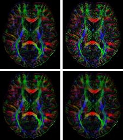
As we are working with real data, we do not have access to an exact solution of the denoising problem. Instead, we used a higher quality reference data set for comparison. This data set was obtained by registering and averaging 18 such acquisitions. The noisy input to the denoising algorithm was a data set with four averaged acquisitions consuming about 20% of the acquisition time, compared to the higher-quality one.

For better evaluation of our denoising algorithm, we have compared our 3D SA-DCT results with those obtained using the total variation PDE-based method reported in (cf. Fig. 6).¹¹ This PDE model is essentially a generalization of the well-known Rudin Osher Fatemi (ROF) model and the Blomgren Chan model.^31,32 The solution here is the minimizer u of an energy functional on the form

16

where R(u) is a regularization functional which measures the smoothness of u, and F(u,f) is a fidelity functional that measures the distance from the noisy data f and the solution u. The solution is a compromise between a completely smooth solution (λ = 0) and a solution that is close to the input data (λ≫0).

Fig 6.

Color-coded FA plot of a slice from the DTI dataset recorded in a healthy volunteer. Upper left panel: high quality scan using 18 averages. Upper right panel: the 4 averaged dataset that was input to the 3D SA-DCT denoising algorithm. Lower left panel: the output of the SA-DCT algorithm. Lower right panel: a comparison image calculated using the PDE technique described in ¹¹.

We calculated the error in the tensor in the same way as in the previous example. Using this measurement, we found the global error of the noisy image (four averages compared to 18 averages) to be 96.61. Denoising with the 3D SA-DCT algorithm was able to reduce the error to 77.07. The PDE denoising algorithm produced a solution with a global error of 76.19.

CONCLUSIONS

In this paper, we have generalized the SA-DCT methods from 2D scalar-valued images via 3D scalar-valued images to 3D tensor-valued images. We have shown numerical experiments on both 3D scalar-valued images and 3D tensor-valued images. The numerical studies indicate that the SA-DCT framework can successfully be applied as an alternative method for denoising in both the scalar-valued setting and the tensor-valued setting.

We have demonstrated that a substantial improvement of results can be achieved by employing the genuine 3D denoising algorithm, as opposed to 2D SA-DCT denoising applied slice-by-slice.

In addition, we have shown that our numerical results are comparable to those obtained with 3-dimensional PDE-based techniques of the kind reported in Christiansen et al.¹¹ That PDE approach represents a class of total variation denoising algorithms that has up to now been considered state-of-the-art. The fact that the 3D SA-DCT approach, representing a mathematically simpler idea, can provide results that are of the same quality is remarkable. Moreover, an important advantage of the SA-DCT is that the method is local in nature. Thus, it is easy to parallelize the algorithm and speed up the calculations. This is a topic for further studies.

We also believe it would be beneficial to extend the method to work directly on the matrix structure instead of its elements; however, this is not a trivial task. The key idea behind the method is to work on homogeneous areas, and how to extend this to matrices is not know. Thus, we have left this as topic for further studies.

We are aware of the sparse data being used for evaluation of our numerical experiments. A natural next step will be to evaluate the performance on a large number of DTI data sets, comparing FA values within specific regions of interest, and also comparing fiber tracking results obtained after PDE-denoising and after SA-DCT denoising of the tensors.

From our preliminary results, we conclude that SA-DCT denoising methods are both well performing and comparable to other methods with respect to computational cost. A parallel implementation of the methodology might as well have a potential in clinical examinations and in biomedical research where DTI data are recorded.

References

- 1.Mori S, Zijl PCM. Fiber tracking: principles and strategies—a technical review. NMR Biomed. 2002;15:468–480. doi: 10.1002/nbm.781. [DOI] [PubMed] [Google Scholar]
- 2.Zhukov L, Barr AH: Oriented tensor reconstruction: Tracing neural pathways from diffusion tensor MRI. in VIS ’02. Proceedings of the Conference on Visualization 2002, pp 387–394, (IEEE Computer Society)
- 3.Basser PJ, Mattiello J, LeBihan D. MR diffusion tensor spectroscopy and imaging. Biophys J. 1994;66:259–267. doi: 10.1016/S0006-3495(94)80775-1. [DOI] [PMC free article] [PubMed] [Google Scholar]
- 4.Basser PJ, Pajevic S, Pierpaoli C, Duda J, Aldroubi A. In vivo fiber tractography using DT-MRI data. Magn Reson Med. 2000;44:625–632. doi: 10.1002/1522-2594(200010)44:4<625::AID-MRM17>3.0.CO;2-O. [DOI] [PubMed] [Google Scholar]
- 5.Niethammer M, San-Jose Estepar R, Bouix S, Shenton M, Westin C-F: On diffusion tensor estimation. Proceedings of the 28th IEEE Engineering in Medicine and Biology Society (EMBS), New York City, 2006, pp 2622–2625 [DOI] [PMC free article] [PubMed]
- 6.Westin C-F, et al. Processing and visualization for diffusion tensor MRI. Med Image Anal. 2002;6:93–108. doi: 10.1016/S1361-8415(02)00053-1. [DOI] [PubMed] [Google Scholar]
- 7.Foong J, et al. Neuropathological abnormalities of the corpus callosum in schizophrenia: a diffusion tensor imaging study. J Neurol Neurosurg Psychiatry. 2000;68:242–244. doi: 10.1136/jnnp.68.2.242. [DOI] [PMC free article] [PubMed] [Google Scholar]
- 8.Goldberg-Zimring D, Mewes AUJ, Maddah M, Warfield SK. Diffusion tensor magnetic resonance imaging in multiple sclerosis. J Neuroimaging. 2005;15:68–81. doi: 10.1177/1051228405283363. [DOI] [PubMed] [Google Scholar]
- 9.Lim KO, et al. Compromised white matter tract integrity in schizophrenia inferred from diffusion tensor imaging. Arch Gen Psychiatry. 1999;56:367–374. doi: 10.1001/archpsyc.56.4.367. [DOI] [PubMed] [Google Scholar]
- 10.Chefd’hotel C, Tchumperlè D, Deriche R, Faugeras O. Regularizing flows for constrained matrix-valued images. J Math Imaging Vis. 2004;20:147–162. doi: 10.1023/B:JMIV.0000011324.14508.fb. [DOI] [Google Scholar]
- 11.Christiansen, O., Lee, T.-M., Lie, J., Sinha, U. & Chan, T.F.: Total Variation regularization of matrix valued images. International Journal of Biomedical Imaging, Volume 2007, Article ID 27432, 11 pages. DOI 10.1155/2007/27432 [DOI] [PMC free article] [PubMed]
- 12.Tschumperle D, Deriche R.: Variational Frameworks for DT-MRI Estimation, Regularization and Visualization. Proceedings of the Ninth IEEE International Conference on Computer Vision (ICCV 2003) Corfu, Greece, 2003
- 13.Wang Z, Vemuri BC, Chen Y, Mareci TH. A constrained variational principle for direct estimation and smoothing of the diffusion tensor field from complex DWI. IEEE Trans Med Imag. 2004;23:930–939. doi: 10.1109/TMI.2004.831218. [DOI] [PubMed] [Google Scholar]
- 14.Weickert J, Brox T. Diffusion and regularization of vector- and matrix-valued images. Universitet des Saarlandes, Fachrichtung 6.1 Mathematic, Preprint No. 58, 2002
- 15.Welk M, et al. Median and related local filters for tensor-valued images. Signal Process. 2007;87:291–308. doi: 10.1016/j.sigpro.2005.12.013. [DOI] [Google Scholar]
- 16.Foi, A: Dipartimento di Matematica, Politecnico di Milano, 2005
- 17.Foi A, Dabov K, Katkovnik V, Egiazarian K: Shape-adaptive DCT for denoising and image reconstruction. Proc. SPIE Electronic Imaging 2006, Image Processing: Algorithms and Systems V. San Jose, California, USA, 2006
- 18.Foi A, Katkovnik V, Egiazarian K: Pointwise shape-adaptive DCT as an overcomplete denoising tool. The International Workshop on Spectral Methods and Multirate Signal Processing, 2005
- 19.Katkovnik V, Egiazarian K, Astola J. Adaptive window size image de-noising based on intersection of confidence intervals (ICI) rule. J Math Imaging Vis. 2002;16:223–235. doi: 10.1023/A:1020329726980. [DOI] [Google Scholar]
- 20.Weickert J, Hagen H: Visualization and processing of tensor fields. Springer, 2005
- 21.Stejskal EO. Use of spin echoes in a pulsed magnetic-field gradient to study anisotropic, restricted diffusion and flow. J Chem Phys. 1965;43:3597–3603. doi: 10.1063/1.1696526. [DOI] [Google Scholar]
- 22.Stejskal EO, Tanner JE. Spin diffusion measurements: Spin echoes in the presence of a time-dependent field gradient. J Chem Phys. 1965;42:288–292. doi: 10.1063/1.1695690. [DOI] [Google Scholar]
- 23.Hahn KR, Prigarin S, Heim S, Hasan K: Random noise in diffusion tensor imaging, its destructive impact and some corrections. Visualization and image processing of tensor fields. Mathematics and Visualization Series 1–13, 2006
- 24.McGraw T, Vemuri BC, Chen Y, Rao M, Mareci T. DT-MRI denoising and neuronal fiber tracking. Med Image Anal. 2004;8:95–111. doi: 10.1016/j.media.2003.12.001. [DOI] [PubMed] [Google Scholar]
- 25.Zhukov L, Barr AH: Heart-muscle fiber reconstruction from diffusion tensor MRI. In: Proceedings of the 14th IEEE Visualization Conference, pp 597–602, 2003
- 26.Sikora T. Low complexity shape-adaptive DCT for coding of arbitrarily shaped image segments. Signal Process Image Commun. 1995;7:381–395. doi: 10.1016/0923-5965(95)00009-9. [DOI] [Google Scholar]
- 27.Sikora T, Bauer S, Makai B. Efficiency of shape-adaptive 2-D transforms for coding of arbitrarily shaped image segments. IEEE Trans Circuits Syst Video Technol. 1995;5:254–258. doi: 10.1109/76.401104. [DOI] [Google Scholar]
- 28.Cocosco CA, Kollokian V, Evans AC: BrainWeb: Online interface to a 3D MRI simulated brain database. NeuroImage 5, 1997
- 29.Kindlmann G: Teem: Tools to process and visualize scientific data and images. http://teem.sourceforge.net/.
- 30.Mori S: DTI-Studio: http://cmrm.med.jhmi.edu/.
- 31.Blomgren P, Chan TF. Color TV: Total variation methods for restoration of vector-valued images. IEEE Trans Image Process. 1998;7:304–309. doi: 10.1109/83.661180. [DOI] [PubMed] [Google Scholar]
- 32.Rudin L, Osher S, Fatemi E. Nonlinear total variation based noise removal algorithm. Physica D. 1992;60:259–268. doi: 10.1016/0167-2789(92)90242-F. [DOI] [Google Scholar]