Automatic Cobb Measurement of Scoliosis Based on Fuzzy Hough Transform with Vertebral Shape Prior

Abstract

To reduce variability of Cobb angle measurement for scoliosis assessment, a computerized method was developed. This method automatically measured the Cobb angle on spinal posteroanterior radiographs after the brightness and the contrast of the image were adjusted, and the top and bottom of the vertebrae were selected. The automated process started with the edge detection of the vertebra by Canny edge detector. After that, the fuzzy Hough transform was used to find line structures in the vertebral edge images. The lines that fitted to the endplates of vertebrae were identified by selecting peaks in Hough space under the vertebral shape constraints. The Cobb angle was then calculated according to the directions of these lines. A total of 76 radiographs were respectively analyzed by an experienced surgeon using the manual measurement method and by two examiners using the proposed method twice. Intraclass correlation coefficients (ICC) showed high agreement between automatic and manual measurements (ICCs > 0.95). The mean absolute differences between automatic and manual measurements were less than 5°. In the interobserver analyses, ICCs were higher than 0.95, and mean absolute differences were less than 5°. In the intraobserver analyses, ICCs were 0.985 and 0.978, respectively, for each examiner, and mean absolute differences were less than 3°. These results demonstrated the validity and reliability of the proposed method.

Introduction

Idiopathic scoliosis (IS) is a three-dimensional lateral curvature of the spine coupled with vertebral rotation for which there is no known cause. About 2–4% of the adolescent population has some degree of scoliosis^1,2. Approximately 2.2% of these adolescents will require treatment, consisting of observation, orthotic (brace) treatment, or surgery³.

If scoliosis is left untreated and a large curve develops, it can injure both the lungs and heart causing significant health problems. Treatment decisions for scoliosis are based on consideration of the patient’s physiologic maturity, curve severity, curve location, cosmetic concerns, and the estimated potential for progression. The Cobb angle method⁴ is the gold standard to measure the curve severity. A Cobb angle less than 10° is not considered to be scoliosis. Spinal deformity with a Cobb angle of 10° to 25° will be monitored regularly until skeletal maturity or significant curve progression. If the Cobb angle is 25° to 45°, brace treatment is suggested. If the Cobb angle is greater than 45°, surgery is usually recommended³. Generally, 5° of change or more between two successive radiographs is considered as the indication of curve progression⁵.

To measure the Cobb angle, the end-vertebrae that tilt most severely toward the concavity of the spinal curve are identified. The Cobb angle can be manually measured by calculating the angle (θ) between the lines respectively drawn along the upper endplate of the superior end-vertebra and the lower endplate of the inferior end-vertebra, as shown in Figure 1. However, the manual measurement of Cobb angle depends on experience and judgment. Errors are due to selecting different end-vertebrae and estimating different slopes of the vertebrae. Even when the same end-vertebrae are used for measurement, the standard measurement error is 3° to 5° for the same observer and 5° to 7° for different observers^5–7, which are beyond the 5° for progression assessment. In addition, the manual measurement is tedious and time-consuming.

Fig 1.

Cobb angle measurement.

Allen et al.⁸ developed an automatic Cobb measurement method based on active shape models, where the training set was required, and the measurement results heavily relied on the training data. Chockalingam et al.⁹ proposed a method to measure the Cobb angle automatically. Their program automatically generated eight horizontal lines over the region of interest (ROI) dividing the spine image into equally spaced regions. Users set two points on each line where it intersected the vertebrae edge. Connecting these midpoints on each of the line defined the midline of the spine. The Cobb angle was calculated based on the midline of the spine. The accuracy of this method depended on how well the edges of the vertebrae were identified. Xu et al.¹⁰ used a similar method, which was based on the spinal midline to measure the Cobb angle. Their method automatically detected the boundary of the spine joining the vertebrae. However, the accuracy of the study has not been reported.

This proposed work is a new approach which incorporates the vertebral shape prior into the fuzzy Hough Transform (FHT)¹¹ to automatically detect the directions of the end-vertebrae on the posteroanterior (PA) radiograph. After the directions of the end-vertebrae were automatically determined, the Cobb angle is calculated. No training set is required, and minimum involvement is needed. The reliability and repeatability of this method was tested by two examiners in a 2-week period. The overall goal of this study was to reduce measurement error of the Cobb angle by reducing the judgment required in measuring the severity of idiopathic scoliosis.

Materials and Methods

Materials

Seventy-six PA radiographs of 71 females and 5 males age 14.7 ± 2.3 who attended one site between April and November 2007 using Fuji CR 5000R computed radiography with 10 pixels/mm resolution were selected. The selection criteria were (1) diagnosis of idiopathic scoliosis, (2) ages between 9 and 18 years, and (3) Cobb angle less than 90°. The exclusion criteria were patients who (1) had other musculoskeletal or neurological disorders, (2) prescribed a brace, or (3) had had surgery. This study received ethics approval from the local ethic board.

The maximum Cobb angle measured by the orthopedic surgeon was 68°. According to the Lenke classification¹², there are 29 cases of type 1, 1 case of type 2, 14 cases of type 3, 16 cases of type 5, and 16 cases of type 6.

Methods

Although a fully automatically method is one of the goals of this study, the developed method still requires the user to select the two end-vertebrae of the curve as well as the brightness and contrast adjustment. As illustrated in Figure 1, once the directions of the lines that fit the endplates of the end-vertebrae (θ₁ and θ₂) are known, the Cobb angle θ can be calculated as θ = θ₁ + θ₂. In this approach, after the end-vertebrae were selected, the directions of these lines were automatically estimated based on fuzzy Hough transform. The developed algorithm was implemented in MATLAB 7.0 and Visual C++.NET. The whole processing procedures are illustrated in the flowchart (Fig. 2).

Fig 2.

Processing procedure.

Preprocessing

Because the quality of the spinal radiographs was inconsistent, and the vertebral sizes were variant in a large range, it was difficult to process the images directly by the computer. Therefore, the original radiograph was cropped from cervical vertebra (C7) to sacrum and was resized to a standard height of 1,000 pixels. Each resized images was manually enhanced by adjusting the brightness and contrast using Image J software [NIH, USA]. The most tilted end-vertebrae were selected from the enhanced images. The regions of interest (ROI of size 100 × 80 pixels, as shown in Figure 3a) containing the selected end-vertebrae were created by the algorithm.

Fig 3.

Preprocessing. a ROIs selection; b denoised ROIs by anisotropic diffusion; c edge detection by Canny operator; d edge images without anisotropic diffusion.

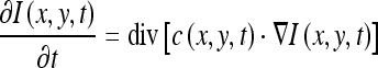
Because the radiograph contains a complex background due to various types of artifacts, it is necessary to denoise the images to facilitate the following processing. The anisotropic diffusion algorithm¹³ can remove noises while preserving edge information. It can be described as the partial differential equation:

1

where I is the image, x and y represent the spatial coordinates of each image pixel, t is artificial time parameter corresponding to the iteration index in the discrete implementation, div represents divergence operator, ▿ is the gradient operator, and c(x, y, t) is the diffusion conductance function, usually defined as

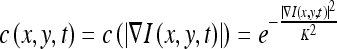2

where K is the relaxation parameter which is chosen according to the noise levels. K was set as 6.0 in the experiments. The diffusion conductance function diffuses more in smooth areas and less across edges. Therefore, the anisotropic diffusion method can realize intra-region smoothing in preference to smoothing across edges. Figure 3b is the denoised images of the ROIs in Figure 3a.

Edge information is a prerequisite to implement the Hough transform. The Canny operator¹⁴ is the most commonly used method and is regarded as optimal for edge detection. The Canny edge detector is then applied to Figure 3b images, and the results are shown in Figure 3c. To illustrate the effect of the anisotropic diffusion, the edge images of the ROIs (without applying the anisotropic diffusion) obtained by the same Canny operator are shown in Figure 3d, where many noisy edges are found.

Fuzzy Hough Transform

Hough transform (HT)^15,16 is originally a technique to detect straight lines. In the image space (x–y plane), any line is represented as ρ = x cos θ + y sin θ, where ρ is the distance between the line and the origin, and θ is the angle of the vector from the origin to the closest point of the line, as illustrated in Figure 4.

Fig 4.

Representation of a straight line.

The (ρ, θ) plane is referred as Hough space. Accordingly, a point (x₀, y₀) in the image space corresponds to a curve ρ = x₀ cos θ + y₀ sin θ in the Hough space, and all the points belonging to a particular line (specified by (ρ₀, θ₀)) correspond to a family of curves passing through a common point (ρ₀, θ₀). Applying the HT to a set of edge points results in a two-dimensional function C(ρ, θ), which represents the number of edge points satisfying the linear equation ρ = x cos θ + y sin θ. In practical applications, the Hough space is quantized and the accumulator array C(ρ_k, θ_k) is obtained. By finding the local peaks of C(ρ_k, θ_k), the most likely lines can be detected.

However, in the conventional HT, even if an edge point is near the line specified by (ρ_k, θ_k), it does not contribute to C for that (ρ_k, θ_k). In other words, there is no difference between a point being far from the ideal line or being just a little off it. Because each side of the vertebra is not exactly a straight line, but is close to a straight line (as shown in Fig. 3c or d), it may be difficult to correctly find out the peaks in the Hough space to specify the line segments that fit to the vertebra sides. Han et al.¹¹ developed the FHT, where around each point on the ideal line a small region R was defined, and each edge point in this region contributed more or less to the accumulator C depending on its distance (d) from the ideal line. Therefore, the peaks could be identified correctly even for distorted line structures. In addition, a faster algorithm¹¹ was proposed to realize the FHT by convolving the accumulator C along the ρ axis with the membership function

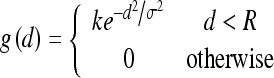3

where k, σ, and R were constants that were chosen empirically as k = 2 and R = σ = 4 in the experiments.

The effectiveness of the FHT is illustrated in Figure 5, where a and d are the edge images, and b, c, e, and f show the detected lines by finding the maximum peaks in Hough space. In Figure 5d, e, and f, one dot represents one edge pixel. Figure 5b and c shows the detected lines of a by using the conventional HT and FHT, respectively, where the lines detected by the FHT are visually more convincing to humans. Figure 5e and f shows the detected lines of d by using the HT and FHT, respectively, where the conventional HT finds seven lines and each one passes through six edge points, while the FHT finds the single line that correctly fits to the edge points.

Fig 5.

Comparison of the conventional HT and FHT: edge images (a) and (d), detected lines of (a) by HT (b) and FHT (c), detected lines of (d) by HT (e) and FHT (f).

If the FHT can detect the line segments that fit the endplates of the end-vertebrae properly, the Cobb angle can be calculated from the directions of these lines as described previously. However, because of the complexity of vertebra images, the FHT sometimes failed to find the proper lines. As an example, Figure 6 shows the edge images of vertebrae (in the upper row) and the incorrect endplates detected by the FHT (in the lower row), where the artifacts from the structure within the vertebra (a), the neighboring vertebra (b), and the background (c) caused the lines (detected by finding the maximum peaks in Hough space) fail to fit to true endplates of the end-vertebrae. Our solution was to incorporate the vertebral shape prior into the FHT.

Fig. 6.

a–c Edge images of vertebrae and incorrect line segments detected by FHT.

Vertebral Shape Prior in Hough Space

Let H₁ = (ρ₁, θ₁), H₂ = (ρ₂, θ₂),…, and H_l = (ρ_l, θ_l) denote the l peaks of C(ρ_k, θ_k). It can be observed that the vertebral sides satisfy the specific geometric relations in Hough space:

1. Let the peaks (ρ_i, θ_i) and (ρ_j, θ_j), respectively, correspond to the upper and lower endplates of a vertebra (the horizontal sides of the vertebra). For a minor-deformed vertebra, θ_i and θ_j are approximately equal, i.e., |θ_i− θ_j| < T₁, (T₁ = 10 is the threshold), as two endplates are almost parallel. Similarly, the pair of peaks corresponding to the vertical sides of the vertebra satisfies the same condition.

2. Let and represent the average θ values of the pairs of peaks that respectively correspond to the horizontal sides and the vertical sides. For a minor-deformed vertebra, , (T₂ = 10 is the threshold), as the horizontal sides and the vertical sides are close to perpendicular to each other.

3. The value of (corresponding to the pair of endplates) is less than 45° (half of 90°), as 45° is considered as the maximum angle of a single tilted vertebra, and 90° is considered as the maximum Cobb angle possibly met with the inclusion criteria of this study.

4. The difference between the ρ values of two peaks that correspond to the endplates is at the range from 30 to 60 pixels, i.e., 30 < | ρ_i− ρ_j | < 60, as the height of the vertebrae in the resized images is within this range. Similarly, the pair of peaks corresponding to the vertical sides satisfies 40 < |ρ_i− ρ_j| < 80.

Automatic Cobb Angle Measurement

Based on the vertebral shape prior, the Cobb angle can be calculated by the following steps.

• Step 1apply the FHT to the edge image. In Hough space, choose the peaks whose C values are beyond 60% of the maximum C value.
• Step 2pair the peaks that satisfy |θ_i− θ_j| < T₁. Let denote the average angle of a pair of peaks, i.e., 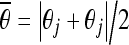. Select the pairs, which satisfy and 30 < | ρ_i− ρ_j| < 60, as the horizontal candidate pairs; select the pairs, which satisfy or and 40 < |ρ_i− ρ_j| < 80, as the vertical candidate pairs. Let and , respectively, denote the average angles of the nth horizontal and vertical candidate pairs.
• Step 3compare all candidate pairs to find those satisfy that . Identify the couple of pairs with the maximum average C values, of which the horizontal pair () is considered as the peaks that correspond to the endplates. The corresponding angle is considered as the angle of the tilted vertebra. The detected line segments that fit to the endplates of the vertebrae in Figure 3c and in Figure 6 are respectively shown in Figure 7.

Fig 7.

a–e Detected vertebra direction and line segments that fit to the endplates of the vertebrae.

Finally, the Cobb angle is calculated as the sum of the angles of two end-vertebrae.

Performance Analysis

The proposed method was tested and compared with the manual measurement method to evaluate its performance. The manual method was measured by an orthopedic surgeon specialized in scoliosis with 25 years experience. Two examiners were respectively asked to measure the Cobb angle on each radiograph by using the developed software twice over a period of 2 weeks. Examiner 1 (E1) was involved in scoliosis clinic for 20 years, and examiner 2 (E2) was the software developer with no clinical experience to measure Cobb angle manually. The results obtained from the surgeon were considered as the true values. All measurements on the same radiograph were performed on the same curve, although some spines had multiple curves.

Spearman correlation studies were used to assess the strength of the relation between two measurements. A higher correlation coefficient (r, varying between 0 and 1) indicates a better linear relation between two measurements. Paired t tests were performed to assess the significance of potential variation between two measurements. A p value (significance level) for Spearman correlation and paired t test was considered significant if less than 0.05. The intraclass correlation coefficient (ICC, varying between 0 and 1) with 95% confidence intervals (CI) was used to evaluate the reliability¹⁷. The Currier criteria¹⁸ for ICC values were adopted: 0.90–0.99 = high reliability, 0.80–0.89 = good reliability, 0.70–0.79 = fair reliability, <0.69 = poor reliability. As an error analysis, mean absolute difference of two measurements was also assessed, with the associated 95% CI. SPSS (SPSS Inc, Chicago, IL, USA) was used to perform these analyses.

Results and Discussion

To evaluate the validity of the proposed method, the automatic measurements from two examiners were respectively compared with the manual measurement from the surgeon. The results were given in Table 1. All Spearman correlation analyses showed r > 0.9 and p < 0.001, which indicated strong correlation between the automatic and manual measurements. The paired t tests results of p > 0.05 suggested that the differences between the manual and automatic measurements were not significant. All ICC values were higher than 0.95, with 95% CI between 0.924 and 0.981. The mean absolute differences between the automatic and manual measurements were all less than 5°, with 95% CI between 2.9° and 5.2°. These results demonstrated high agreement of the automatic method with the manual measurement method. These results also indicated that using the automatic method could obtain the similar results even by the examiner with little experience.

Table 1.

Comparison Between Automatic and Manual Measurements

Parameter		Spearman correlation		Paired t test	ICC (95% CI)	Mean absolute difference (95% CI)
		r	p	p
E1 vs. S	First	0.943	<0.001	0.079	0.970 (0.953, 0.981)	3.6° (3.0°, 4.2°)
	Second	0.935	<0.001	0.051	0.967 (0.947, 0.979)	3.8° (3.1°, 4.5°)
E2 vs. S	First	0.935	<0.001	0.578	0.966 (0.946, 0.978)	3.6° (2.9°, 4.3°)
	Second	0.909	<0.001	0.280	0.952 (0.924, 0.969)	4.4° (3.6°, 5.2°)

The results of the interobserver reliability analyses were presented in Table 2. It was shown that the measurements from two examiners were highly correlated with each other (r > 0.9 and p < 0.001). The paired t tests results of p > 0.05 indicated that the interobserver differences were not statistically significant. The ICCs > 0.95, with 95% CI between 0.945 and 0.982, showed high interobserver reliability. The mean absolute differences were less than 5° with 95% CI between 2.7° and 4.6°. These results suggested that the automatic method was consistent regardless of the experience of the examiners.

Table 2.

Interobserver Analyses

E1 vs. E2	Spearman correlation		Paired t test	ICC (95% CI)	Mean absolute difference (95% CI)
	r	P	p
First	0.945	<0.001	0.240	0.972 (0.956, 0.982)	3.4° (2.7°, 4.0°)
Second	0.934	<0.001	0.144	0.965 (0.945, 0.978)	3.9° (3.2°, 4.6°)

The intraobserver reliability of the proposed method was assessed for each examiner. The results were presented in Table 3. The Spearman correlation results of r > 0.9 and p < 0.001 showed strong correlation between the measurements by the same examiner. The paired t tests results of p > 0.05 indicated that the measurements by the same examiner were not significantly different. Both intraobserver analyses produced ICCs > 0.95, with 95% CI between 0.966 and 0.990. The mean absolute differences were less than 3° with 95% CI between 2.1° and 3.5°. These results demonstrated high intraobserver reliability of the proposed method.

Table 3.

Intraobserver Analyses

Parameter	Spearman correlation		Paired t test	ICC (95% CI)	Mean absolute difference (95% CI)
	r	p	p
E1	0.971	<0.001	0.143	0.985 (0.976, 0.990)	2.5° (2.1°, 3.0°)
E2	0.958	<0.001	0.282	0.978 (0.966, 0.986)	2.9° (2.3°, 3.5°)

To investigate whether the severity of the curve would affect the automatic measurement, the radiographs were classified into three categories according to the Cobb angle measured by the surgeon: less than 25° (13 radiographs), between 25° and 45° (49 radiographs), and more than 45° (14 radiographs). The comparison between the manual and automatic measurements was then performed on three categories, respectively. All Spearman correlation analyses resulted in p < 0.001, which indicated that there was a strong correlation between the automatic and manual measurements regardless of the curve severity. The paired t tests results of p > 0.05 indicated that the intermethod differences were not statistically significant in any of the three categories. The ICCs and mean absolute differences were presented in Tables 4 and 5, respectively. It was shown in Table 4 that the lowest ICC value was 0.768 in the category of curve between 25° and 45°, and the highest ICC value was 0.953 in the category of curve more than 45°. Although the ICC values were different, the results still indicated that the severity of the curve did not cause the significant differences to the intermethod measurement. The mean absolute differences in Table 5 showed that the intermethod differences were still within 5° for any of the three categories. In the comparison between the automatic measurement from the E2 (no clinical experience) and the manual measurement from the experienced surgeon, the mean absolute differences was 5° in the category of curve more than 45°. It might be due to the selection of different vertebrae between the E2 and the surgeon.

Table 4.

ICCs (95% CI) of Intermethod for Three Categories of Curves

Curve Category		Less than 25°	Between 25° and 45°	More than 45°
E1 vs. S	First	0.874 (0.586, 0.961)	0.830 (0.699, 0.904)	0.925 (0.765, 0.976)
	Second	0.910 (0.704, 0.972)	0.777 (0.605, 0.874)	0.953 (0.853, 0.985)
E2 vs. S	First	0.912 (0.713, 0.973)	0.848 (0.730, 0.914)	0.908 (0.712, 0.970)
	Second	0.887 (0.631, 0.966)	0.768 (0.588, 0.869)	0.875 (0.611, 0.960)

Table 5.

Mean Absolute Difference (95% CI) of Intermethod for Three Categories of Curves

Curve Category		less than 25°	between 25° and 45°	more than 45°
E1 vs. S	First	2.9° (1.4°, 4.5°)	3.7° (2.9°, 4.4°)	3.9° (2.2°, 5.6°)
	Second	2.5° (1.2°, 3.8°)	4.2° (3.2°, 5.2°)	3.6° (2.3°, 4.9°)
E2 vs. S	First	2.5° (1.6°, 3.4°)	3.5° (2.8°, 4.3°)	4.1° (2.3°, 5.9°)
	Second	3.1° (2.2°, 3.9°)	4.4° (3.4°, 5.3°)	5.0° (3.9°, 7.2°)

Currently, both of the manual and the proposal methods depended on the quality of the radiographs. User’s manual adjustment to get good brightness and contrast images was required. The end-vertebrae selection was the relatively simple step during the user judgment. The manual method then required the user to draw two straight lines to pass through the end-plates of the vertebrae, but the computer algorithm automatically calculated the Cobb angle. The average computing time was less than half a minute after two end-vertebrae were selected. This was similar to the time that an experienced surgeon would need to determine the Cobb angle from a radiograph using the manual method. However, the computer method resulted in a smaller variability.

The proposed method required less user intervention, compared with the computerized method proposed by Chockalingam et al.⁹ where at least 16 points must be assigned manually to define the vertebral edges. Compared with another computerized method proposed by Allen et al.⁸, the proposed method did not require the training set. As long as each individual vertebra tilted less than 45°, the accuracy of the proposed method had no relations with the severity of the spinal curve. Although the shape constraints were reasonable for most radiographs, false detection might occur if a vertebra tilted more than 45°, or the vertebra had a severely deformed shape that did not satisfy the shape constraints. Although some of the endplates of vertebrae were more like a plate, as long as the two vertical sides of the vertebra were still close to parallel, the direction of the vertebra might be detected correctly. The algorithm would choose the most fitted couple of pairs of lines, which improved its robustness.

Conclusion

Although the proposed method still required user judgment to measure the Cobb angle, very little user interaction and skills are required. Manually drawing lines across the endplates of the end-vertebrae may be the major source for measurement errors. In the proposed method, the directions of these lines were automatically estimated to reduce the errors. The validity analyses demonstrated that this method highly agreed with the manual measurement method. The interobserver and intraobserver analyses indicated that the measurement errors were comparable to the threshold of changes that could influence treatment decisions. These results suggested that the proposed method could help orthopedic surgeons measure the Cobb angle more reliably and release their time during scoliosis clinic.

References

- 1.Yawn BP, Yawn RA, Hodge D, Kurland M, Shaughnessy WJ, Ilstrup D, Jacobsen SJ. A population-based study of school scoliosis screening. JAMA. 1999;282:1427–1432. doi: 10.1001/jama.282.15.1427. [DOI] [PubMed] [Google Scholar]
- 2.Rogala EJ, Drummond DS, Gurr J. Scoliosis: incidence and natural history. A prospective epidemiological study. J Bone Joint Surg Am. 1978;60:173–176. [PubMed] [Google Scholar]
- 3.Lonstein JE. Adolescent idiopathic scoliosis. Lancet. 1994;344:1407–1412. doi: 10.1016/S0140-6736(94)90572-X. [DOI] [PubMed] [Google Scholar]
- 4.Cobb JR. Outline for the study of scoliosis. Am Acad Orthop Surg Inst Course Lect. 1948;5:261–275. [Google Scholar]
- 5.Morrissy RT, Goldsmith GS, Hall EC, Kehl D, Cowie GH. Measurement of the Cobb angle on radiographs of patients who have scoliosis. Evaluation of intrinsic error. J Bone Joint Surg Am. 1990;72:320–327. [PubMed] [Google Scholar]
- 6.Pruijs JEH, Hageman MAPE, Keessen W, Meer R, Wieringen JC. Variation in Cobb angle measurements in scoliosis. Skelet Radiol. 1994;23:517–520. doi: 10.1007/BF00223081. [DOI] [PubMed] [Google Scholar]
- 7.Greiner KA. Adolescent idiopathic scoliosis: radiologic decision-making. Am Fam Phys. 2002;65:1817–1822. [PubMed] [Google Scholar]
- 8.Allen S, Parent E, Khorasani M, Hill DL, Lou E, Raso JV. Validity and reliability of active shape models for the estimation of Cobb angle in patients with adolescent idiopathic scoliosis. J Digit Imaging. 2007;0:1–11. doi: 10.1007/s10278-007-9026-7. [DOI] [PMC free article] [PubMed] [Google Scholar]
- 9.Chockalingam N, Dangerfield PH, Giakas G, Cochrane T, Dorgan JC. Computer-assisted Cobb measurement of scoliosis. Eur Spine J. 2002;11:353–357. doi: 10.1007/s00586-002-0386-x. [DOI] [PMC free article] [PubMed] [Google Scholar]
- 10.Xu Z, Pan J, Zhang S: A novel automatic framework for scoliosis x-ray image retrieval. IJCNN 2007, Oriando, Florida, USA, pp 2482–2485
- 11.Han JH, Koczy LT, Poston T. Fuzzy Hough transform. Pattern Recogn Lett. 1994;15:649–658. doi: 10.1016/0167-8655(94)90068-X. [DOI] [Google Scholar]
- 12.Lenke LG, Betz RR, Harms J, Bridwell KH, Clements DH, Lowe TG, Blanke K. Adolescent idiopathic scoliosis: a new classification to determine extent of spinal arthrodesis. J Bone Joint Surg AM. 2001;83:1169–1181. [PubMed] [Google Scholar]
- 13.Perona P, Malik J. Scale-space and edge detection using anisotropic diffusion. IEEE Trans Pattern Anal Mach Intell. 1990;12:629–639. doi: 10.1109/34.56205. [DOI] [Google Scholar]
- 14.Canny J. A computational approach to edge detection. IEEE Trans Pattern Anal Mach Intell. 1986;8:679–714. doi: 10.1109/TPAMI.1986.4767851. [DOI] [PubMed] [Google Scholar]
- 15.Hough PVC: Method and means for recognizing complex patterns. U.S. Patent 3069654, 1962
- 16.Duda RO, Hart PE. Use of the Hough transform to detect lines and curves in pictures. Commun Ass Comput Mach. 1972;15:11–15. [Google Scholar]
- 17.Shrout P, Fleiss J. Intraclass correlations: uses in assessing rater reliability. Psychol Bull. 1979;68:420–428. doi: 10.1037/0033-2909.86.2.420. [DOI] [PubMed] [Google Scholar]
- 18.Currier DP. Elements of research in physical therapy. Baltimore: Williams and Wilkins; 1990. [Google Scholar]