An Artificial Immune-Activated Neural Network Applied to Brain 3D MRI Segmentation

Abstract

In this paper, a new neural network model inspired by the biological immune system functions is presented. The model, termed Artificial Immune-Activated Neural Network (AIANN), extracts classification knowledge from a training data set, which is then used to classify input patterns or vectors. The AIANN is based on a neuron activation function whose behavior is conceptually modeled after the chemical bonds between the receptors and epitopes in the biological immune system. The bonding is controlled through an energy measure to ensure accurate recognition. The AIANN model was applied to the segmentation of 3-dimensional magnetic resonance imaging (MRI) data of the brain and a contextual basis was developed for the segmentation problem. Evaluation of the segmentation results was performed using both real MRI data obtained from the Center for Morphometric Analysis at Massachusetts General Hospital and simulated MRI data generated using the McGill University BrainWeb MRI simulator. Experimental results demonstrated that the AIANN model attained higher average results than those obtained using published methods for real MRI data and simulated MRI data, especially at low levels of noise.

INTRODUCTION

In today’s clinical settings, biomedical imaging has become a standard tool used in different diagnostic fields,^2–7 radiation therapy^8,9 and surgical planning.^10–12 The increased availability of biomedical imaging data permits routine noninvasive examination of patients to characterize brain structures and cerebral and spinal vasculature in aging and neurological disease states. However, the accurate reproducible interpretation of biomedical imaging studies, which is performed visually by highly trained physicians, remains an extremely time-consuming and costly task.¹³ For the purpose of aiding physicians in the interpretation of biomedical imaging studies, several techniques have been proposed for the segmentation of biomedical images, including model-based,^14,15 Kohonen neural networks,¹⁶ regression analysis image scatter charts,¹⁷ energy functional,¹⁸ and statistical or k-nearest neighbor classification.^19,20 Based on the wealth of image processing techniques developed for both biomedical and nonmedical images, several projects have been developed for brain segmentation of Magnetic Resonance (MR) images, e.g., the Internet Brain Segmentation Repository (IBSR),¹⁰⁷ image registration of multiple modalities, e.g., Automatic Image Registration (AIR),²¹ and anatomical reconstruction, e.g., Computerized Anatomical Reconstruction and Editing Toolkit (CARET).²²

Segmentation of MR imaging studies has been achieved based on different schemes for both single-channel and multi-channel data (T1, T2, PD)²³ including techniques based on neural networks,^24–28 classification techniques,^29–33 or predefined models/knowledge.^34,35 The application of segmentation techniques to MR images of the brain can be broadly classified into two categories. In the first category, segmentation is mainly based on the direct use of the intensity data contained in the MR images, with the goal of quantifying global and regional brain volumes, i.e., white matter, gray matter, and/or cerebro-spinal fluid (CSF) volumes, from high-resolution MR images. Examples of approaches from this category include techniques that involve fitting a Gaussian or polynomial model to the data.^89–92 Because of the sensitivity of the Gaussian fitting to noise, which results in speckled regions in the segmentation, Markov Random Field (MRF) models are sometimes combined with the fitting in the segmentation process.^93–100 In the second category, segmentation is performed in conjunction with ideal prior segmentations for the purpose of guiding the segmentation process. This category is composed of model-based (or atlas-based) techniques that typically require images to be coregistered to a segmented standard model image of the brain.^96,103 The registration aims to find a non-rigid transformation that maps the standard brain to the specimen to be segmented. The transformation is then used to segment the brain specimen into the constituent tissues. In both categories, the segmentation could be automated^90,96,97 or semiautomated and typically involves several steps, such as preprocessing of the data, segmentation, normalization, and in some schemes, quantification of regional volumes within a stereotaxic coordinate system.^36,37 Brain volumetric measurements, based on both categories of techniques, have been correlated with clinical measures and are being used with increasing frequency as objective markers of aging and disease states. For example, cross-sectional and longitudinal differences in brain structure during aging,³⁸ prediction of Alzheimer’s disease,⁴⁰ pretreatment evaluation of patients with temporal lobe epilepsy,³⁹ objective measures of disease severity and progression in multiple sclerosis^41–44 and brain parenchymal volume,^45,46 and evidence of degeneration of extra-motor and frontal gray matter in patients with Amyotrophic Lateral Sclerosisw (ALS) and of the corticospinal tract in the subset of patients with bulbar-onset ALS.⁴⁷

Published studies^1,44,51 suggest that co-analysis of segmented MR imaging data and functional MR data can improve the accuracy of assessing the burden of disease in patients with neurodegenerative, inflammatory/infectious, and neurovascular disorders. In these studies, segmented high-resolution 3-dimensional (3D) (or 2-dimensional) MR anatomical images are co-analyzed with functional MR data sets such as spectroscopic imaging, magnetization transfer imaging, diffusion-weighted imaging, perfusion imaging, other neuroimaging studies, e.g., positron emission tomography, or a coregistered digital stereotaxic atlas of neuroanatomy.⁴⁸ The goal in these studies is usually to generate tissue-specific or region-specific functional results, thereby improving sensitivity and accuracy of the functional measurements. For example, variation of in vivo metabolite distributions in the normal human brain between gray and white matter and among frontal, parietal, and occipital lobes,^49,50 more accurate discrimination between Alzheimer’s disease subjects and control subjects⁵¹ or neurodegenerative diseases such as ALS,⁵³ atrophy correction of positron emission tomography (PET)-derived cerebral metabolic rate for glucose consumption in Alzheimer’s disease patients and controls,⁵² and improved understanding of the course of multiple sclerosis and new prognostic information regarding lesion formation based on magnetization transfer histogram analysis of segmented normal-appearing white matter.⁴⁴

The evaluation of other central nervous system (CNS) structures, especially cerebral or spinal vessels, can also benefit from the application of segmentation techniques to MRI data sets. Contrast-enhanced 3D MR angiography, using a gadolinium-chelate contrast agent injected intravenously, is a widely used method for noninvasive evaluation of the carotid and vertebral arteries, and to a lesser extent the intracranial circulation and the spinal intradural vessels.⁵⁴ High-resolution steady state MR angiography images, suitable for detection of millimeter-sized CNS vessels, have simultaneous enhancement of both the artery and vein blood pools. Consequently, separation of arteries and veins is an emerging challenge in magnetic resonance angiography (MRA) analysis.⁵⁵ Because of the complexity of the vascular structure, manual approaches to cerebrospinal vascular tree analysis are impractical, and highly automated vessel segmentation and display methodology have recently been proposed.^56,57

In this paper, an Artificial Immune-Activated Neural Network (AIANN) model is presented and applied to 3D MRI brain segmentation. The AIANN model aims to perform biomedical imaging data classification based on artificial immune functional capabilities, due to their attractive discrimination, robustness, and convergence characteristics. The AIANN model builds on our previous work in Boolean Neural Networks,^64–73 which seek to perform Boolean logic transformations and have been applied for different applications.^58–63 Like other classification approaches, the AIANN model aims to establish a robust mapping of the biomedical imaging data sets into a domain where the overlapping among the different classes or tissues represented by the data is greatly reduced. What differentiates the AIANN is the development of a classification scheme that is conceptually based on the biological immune system functions, which enables dynamic learning, storage of domain knowledge and robust discrimination among classes. The classification process is modeled after the bonding process between receptors and epitopes that is controlled through an energy function measure to ensure accurate recognition. The artificial immunology fundamentals motivating the classification process in the AIANN model will be presented in “Artificial Immunology” section. Then, the AIANN model is introduced, along with the theoretical foundation establishing its characteristics, in “AIANN Model” section, including the context for its application to MRI segmentation. This is followed by the presentation of the preprocessing steps of the 3D MRI data in “Preprocessing” section. Experimental results involving the application of the AIANN model to the 3D segmentation of both real and simulated MRI data sets are provided in “Experimental Results” section. This is followed by the conclusion in “Conclusion” section.

ARTIFICIAL IMMUNOLOGY

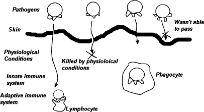
In the past few years, several research efforts have been devoted to biologically inspired systems, including artificial neural networks, evolutionary computation, DNA computation, and artificial immunology systems. The immune system is a complex distributed structure, formed of cells, molecules, and organs,⁸⁶ whose main function is to defend the body against outsider cells attacking the body, or from internal carcinogenic cells. The distributed and logically multilayered nature of the immune system is depicted in Figure 1.

Fig 1.

Logically multi-layered biological immune system.

When a pathogen attempts to enter the body from outside, the first line of defense is the skin. If the pathogen was able to pass through the skin, it is met with the harsh physiological conditions inside the body caused by alkalinity of the mouth, high acidity of the stomach, or higher raised temperature of the body compared to the outside. If the pathogen survives these conditions, it encounters the innate immune system, which arms human beings when born, where phagocytes, which are large white blood cells capable of swallowing the pathogen, can destroy the pathogen. If the pathogen penetrates the innate immune system, it faces the adaptive or acquired immune system. If the adaptive immune system was able to recognize the pathogen, white blood cells, called lymphocytes, secrete enzymes that cause lysis to the cellular wall of the pathogen, rupturing them and dispelling the cellular fluid, thus causing the destruction of the pathogen. In the context of this recognition process, the adaptive immune system exhibits many desirable properties including discrimination of pathogens with a very high accuracy, selection of a suitable response, information retention or memory, and distributed processing. Artificial Immunology is the field concerned with developing computational models that mimic the biological immune system, similar to Artificial Neural Networks modeling biological neural networks. Based on biological immune principles, new computational techniques have been developed for tackling problems in various disciplines such as optimization,^75,76 pattern recognition,^77,78 neural network approaches,^79–82 data clustering,^83,84 classification on resource-limited basis,^104–106 intrusion detection,⁸⁸ and many other fields.⁸⁵

The ability of the immune system to recognize and differentiate between self cells, those belonging to the body, and non-self cells, those that do not belong to the body, results from a training period taking place in the thymus where immune cells that recognize self-proteins are killed.⁸⁷ The training period is termed the tolerization period and the process is called negative selection. Recognition of cells takes place through bonding between the molecules on the surface of the lymphocyte and those on the surface of the pathogen.⁸⁷ Bonding takes place through protein structures on both surfaces that are called receptors on the surface of the lymphocyte and epitopes on the surface of the pathogen. During negative selection, a large number of lymphocyte cells are generated and kept for a certain amount of time inside the lymph nodes. If during that time the lymphocyte bonds to self-cells it is killed and never allowed to flow into the blood stream. Recognition takes place when enough bonds are created between the lymphocyte and non-self cells, with the number of bonds varying among different lymphocytes.

Several attractive properties of biological immunology lay the foundation of effective mechanisms for handling computational and modeling problems.^75,88 In the context of this paper, the following properties are of interest:

• Recognition: The ability of the immune system to recognize, and differentiate between the self and non-self cells, which enables the immune system to attack cells that do not belong to the body.

• Memory: The ability of the immune system to retain old knowledge while adding new information about diseases and infections. The adaptive immune system can learn through vaccines and old infections and retain the learned knowledge to be used later in the generation of the correct lymphocytes.

• Specificity versus Generality: The immune system cells can be specific to recognize a short range of pathogens and initiate correct response. On the other hand, some of cells can be generic to recognize a wide range of pathogens, but cannot initiate the correct response, leaving that to other cells. The AIANN model is primarily concerned with the identification of members of a certain class or tissue, i.e., the interest is in specificity rather than generality. In other words, the model of the immune system must be capable of identifying the class of a certain member (identification of a cell as a specific pathogen) rather than just identifying that a member is known (generic identification of a cell as a pathogen).

AIANN Model

The AIANN model presented in this paper builds on the Boolean Neural Networks (BNN) whose algorithm^65,72 ensures the transformation of any Boolean function to a threshold function using simple integer weights with guaranteed convergence characteristics. The BNN has since been applied to a number of problems and has been shown to be qualitatively equivalent to existing neural networks while performing a given task at a much faster rate. The simplicity of the network and its integral weights have also enabled it to be easily implemented in hardware.^66,67 The BNN was successfully used for feature recognition,⁶⁴ supervised classification using the Nearest to an Exemplar (NTE) classifier,⁶⁷ optimization,^68,69 nonparametric supervised classification using the Boolean K-Nearest neighbors (BKNN) classifier,⁷⁰ hierarchical clustering,⁷¹ and MRI segmentation and labeling using a Constraint Satisfaction Boolean Neural Network (CSBNN).⁷³

Definition of Classification Problem

The classification problem is informally defined in terms of the ability to discriminate between members of different joint or disjoint classes in a given representation domain. Given a set of input vectors ν_i, representing feature points in a specific representation domain, classification can be formally defined as the search for a transform, τ_c, that maps all the members of a class c among the input vectors, to a one-dimensional domain λ, λ = τ_c (ν_i), where class c is completely or partially confined to an interval [a_c, b_c] that minimizes the probability of misclassification of that class. Meanwhile, the transform τ_c would map the members of other classes to anywhere outside the interval [a_c, b_c] so that the members of class c can be separated by applying τ_c and conditionally testing the result to be inside [a_c, b_c]. Different artificial immune models use different forms to represent that transformation including Euclidean distance, Hamming distance,¹⁰² and other functions applied using a vector representation of the center of the class and possibly a radius. Selecting a particular transformation is affected by how well it can tolerate noise, and how well it can separate vectors from a certain class that gets embedded in the range of another.

The recognition property of artificial immune models enables the formulation of transformations or neuron activation functions to differentiate between different classes while the memory property is important to the incremental learning process. The term non-self set will be used to describe the class to be recognized, and self set will be used to describe members that belong to all other classes to be rejected. If the transformation can separate most of the self set leaving little overlap between the self and the non-self sets, this results in minimum false positives or non-self vectors classified to the self set. For more than one class, searching for more than one transformation is required, with each separating the members of a certain class from all other classes with the least possible overlaps, thus, achieving the best possible classification.

In AIANN, a logical model is developed for the chemical reactions taking place between receptors and epitopes. Then, the logical model is used as the transformation needed to classify different input vectors belonging to different classes. All artificial immune models present similar logical models for the chemical reaction between receptors and epitopes. The logical model is in the form of bitwise exclusive-OR (XOR) functions between the binary representations of the receptors and the epitopes.¹⁰¹ In artificial immune models, the output of the logical reaction is usually a permutation of the input vector that is intended to minimize the overlap between the input vectors belonging to different classes. After the permutation, a measure is utilized to estimate the distance between the permuted input and each class. A random number generator seeded with the integer equivalent of the permuted input vector may be used.¹⁰¹ Other models have used the r-contiguous bits match¹⁰² and the hamming distance match to measure the distance between the permuted input and each of the classes. However, several concerns are not addressed in existing artificial immune models. First, the mutual dependence between different features used in constructing the input vectors is ignored in the logical reaction or permutation step. Second, the conversion to integer or binary representations of the features results in a loss of accuracy caused by the truncation of the fractional portion of the features representing the input vectors to be classified. Third, the measurement of the distance between the input vector and each class does not consider the codependence of the different features in the input vectors. The AIANN model involves a transformation to separate members of the different classes that aims to address these issues as detailed in the following section.

Modeling the Biochemical Reactions between Epitopes and Receptors

The term detector will be used to refer to the mathematical model of the receptor. Recognition takes place when the number of bonds between the epitopes and the detectors is large enough to warrant detection, i.e., larger than a threshold specific to each lymphocyte. Bonds take place between the atoms of molecules by sharing electrons in covalent bonds or moving electrons in ionic bonds. The bonding either results in releasing energy out of the pair of molecules, i.e., exothermic reactions, or requires adding energy to the pair of molecules, i.e., endothermic reactions. Most of the reactions have initial conditions in the form of sufficient heat being available in the medium or some form of catalyst being present to lower the starting energy conditions of the reaction. Similar to these natural immune concepts, an analogous logical reaction is modeled, in which logical molecules are composed of binary vectors constructed from strings of ones and zeroes rather than atoms. The energy is modeled through intrinsic energies assigned to the ones and zeroes at every position within the molecule to distinguish variations of energy among the atoms. Assuming that the intrinsic energies of a 1 and a 0 at bit position i of the molecule are w_1i and w_0i, respectively, the energy of a logical molecule M composed of L atoms can be expressed as:

1

For a pair of bonding molecules D and P, through an endothermic reaction, the energy after the reaction is higher than the energy before the reaction, as follows:

2

The reverse relationship is true in the case of an exothermic reaction. However, for a chemical reaction to occur, corresponding atoms in a pair of molecules form a bond if certain initial conditions are met. Similarly, a logical function is utilized in the artificial immune model to determine whether a pair of bits (or atoms) in two logical molecules can form a bond. The logical bonding function B(D_i, P_i) between corresponding bits is true, i.e., is equal to 1, if the two bits can bond and is false, i.e., is equal to 0, when the two bits cannot bond. During chemical bonding, the exchange or sharing of an electron or more will change the energies of both atoms involved in the reaction. This is modeled in the logical reactions by changing both corresponding bits that will bond to the pattern of higher energy in case of endothermic reaction or the pattern of lower energy in case of an exothermic reaction.

In summary, bonding between two logical molecules D and P proceeds, depending on the nature of the chemical reaction, i.e., endothermic or exothermic, according to the following sequence:

• For each corresponding pair of bits D_i and P_i in the two molecules, evaluate the bonding function

  3
• If B(D_i, P_i) is equal to one at any bit position i:

  4

  5

The change of the atoms is performed towards the bit pattern of higher or lower intrinsic energy depending on whether the reaction is endothermic or exothermic, respectively. For the purpose of classification, the two molecules involved in the reaction will represent the detector and the epitope.

AIANN Classification

In the context of the biological immune system, recognition is accomplished through a lymphocyte realizing that a cell in contact does not belong to the body when the number of bonds between the receptors and epitopes is larger than a threshold specific to each lymphocyte. In the artificial immune model, the purpose is to recognize the input feature vectors (or epitopes) of multiple classes. Hence, multiple detectors are generated for each class during the training (or tolerization) stage, where the goal is to enhance the recognition of vectors belonging to a class by detectors belonging to that specific class while dampening the ability of detectors belonging to other classes for recognizing the same vectors. Since the input feature vectors representing the classification domain should be generic enough to enable tackling of various problem domains, the above described artificial immune model needs to be extended beyond binary input vectors to address floating point data. This entails the utilization of a continuous differentiable parameter model, which leads to greater accuracy by allowing the model parameters to attain continuous values and to faster training through the generalized probabilistic descent.

The extension of the model starts with the formulation of the bonding function B that represents one of the 16 possible Boolean functions of two variables that represent bonding of corresponding atoms or bits of the detector molecule D and the epitope molecule P, which can be expressed as:

6

In this Boolean function, the restriction of binary parameters a_i, b_i, c_i, d_i, D_i, P_i, can be relaxed to allow the use of real-valued parameters if the comparison operator that results in a true or false value is modeled by a value of 1 to represent the true condition and a value of 0 to represent the false condition. In this context, a sigmoid function S(a–b) can be used to model the comparison operator or the Boolean condition since S approaches 1 when a >> b and approaches 0 when a << b. Alternatively, the sigmoid function can be viewed as the continuous approximation of a unit step and the continuous and differentiable approximation of the comparison operator. Hence, the if conditions comparing w_1i and w_0i can be expressed as:

7

where C_xi is the comparison indicating that . Based on this representation of the comparison operator, the corresponding bits (or atoms) of the detector and epitope molecules after bonding can be expressed as follows for an endothermic reaction:

8

Meanwhile, the corresponding bits of the detector and epitope molecules after bonding can be expressed as follows for an exothermic reaction:

9

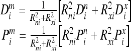
In the proposed AIANN model, more accurate classifications may be attainable when a mixture of both endothermic and exothermic reactions is assumed, i.e., better classification is generated if the transformation involves a mixture of endothermic and exothermic reactions. The mixture bonding reaction model involves the following normalized representation of the corresponding atoms after bonding:

10

where R_ni and R_xi are the relative mixture weighing parameters.

Consequently, the change in energy due to bonding for bit i can be derived by substituting Eqs. (8) and (9) into Eq. (10), formulating the energy after bonding for the detector and epitope based on Eq. (1) and subtracting the energy before bonding formulated for D_i and P_i based on the same Eq. (1). The change in energy for bit i, denoted δE_i, can be expressed as:

11

The overall change in energy for all the atoms as a result of bonding between the epitope and detector j of class k of the artificial immune classification model can be expressed as:

12

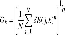
To arrive at an accurate classification, the class to which the input vector or epitope belongs should show a change of energy that exceeds the largest change achieved by any of the detectors of all the other classes. To mathematically represent this relationship in a differentiable form that facilitates the derivation of the training algorithm for generating detectors, the maximum (or max) operator must be represented in a differentiable form as follows:

13

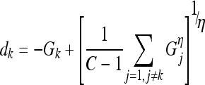
G_k approaches max[δE(j, k)] as η→∞, where N is the number of detectors for class k. To enhance the detection of class k to which the epitope belongs and weaken the ability of other classes’ detectors to bond with the epitope, a decision function d_k is formulated to express the separation between the highest energy change resulting from bonding with any of the class k detectors and the highest change of energy resulting from bonding with any of the detectors of all other classes. The decision function d_k is expressed as follows:

14

where C denotes the total number of classes and the second term in d_k is the continuous representation of the max operator of all the detectors of all the other classes. The decision function acquires a more negative value as the classification is more accurate since the separation in this case is maximized.

Model Stability and Convergence

Based on the decision function, a corresponding loss function l_k can be formulated that approaches zero the more negative the decision function becomes, i.e., l_k approaches zero as the classification becomes more accurate. The loss function l_k is defined as follows:

15

where S is the sigmoid function.

The training of the artificial immune computational model for classification involves searching for the model parameters that lead to robust classification that minimizes the classification errors of the input feature vectors representing epitopes among the classes. It was shown that a local minimization criterion of the following form:

16

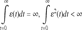
where Λ is the set of model parameters that describe the current state of the classifier and ɛ is the learning rate, will reach a local minimum for the loss function l_k , described by state Λ*, with a probability of one. This minimization criterion has a high probability of reaching the global minimum for low values of the slope of the sigmoid function used in computing the loss. The convergence is conditional on the learning rate ɛ having an infinite integration and the squared value of the learning rate ɛ² having a finite integration over time (or across iterations), which can be expressed as follows:

17

A time decreasing learning rate is more advantageous since a lower learning rate enables fine tuning the parameters around local/global minima as time grows, i.e., as more iterations are involved. The learning rate utilized in the context of the artificial immune computational model is defined as follows to satisfy both conditions:

18

19

This learning procedure is one of the discriminative training algorithms that is commonly called MCE (Minimum Classification Error) and has been widely used for training Hidden Markov Models (HMM). Discriminative training algorithms are primarily concerned with training the classifier to recognize specific data sets while rejecting other datasets. When a given epitope vector is presented to the classifier for training, the parameters of the detectors belonging to the corresponding class and the parameters of the detectors of all the other classes are updated. This, in turn, enhances the recognition of the epitope by the detectors of the class to which it belongs and amplifies the rejection by the detectors of all other classes. Moreover, discriminative training is widely recognized for its speed and convergence and is the least affected by non–infinite training sets^111,112.

The artificial immune classifier parameters that are to be updated per bit for each detector during the learning process are a_i, b_i, c_i, d_i, D_i,w_1i,w_0i,R_xi, R_ni. Each parameter v from this set of parameters is updated by calculating ∇l_k, which in turn requires the evaluation of the partial derivative of the loss function l_i with respect to the parameter v. If v is a parameter of bit i of detector j for class k to which the training epitope vector belongs, ∇l_k is given by:

20

while if the training epitope vector does not belong to class k, ∇l_k is given by:

21

The partial derivatives in Eqs. (20) and (21) can be expressed independent of the parameter v, except for the last one in each equation, as follows:

22

23

24

25

26

The last partial derivative in Eqs. (20) and (21) is dependent on the parameter v being updated. For example, this partial derivative for the detector bit D_i is expressed as:

27

where

28

Based on this foundation for the training process, the procedure involved in the training of an AIANN for C classes, which are known a priori, involving N detectors per class proceeds as follows:

1. Average Loss = Any value greater than 1

2. Total Loss = 0

3. Iterations = 0

4. WHILE Iterations < Maximum AND Average Loss > Minimum_Required

   1. Find the learning rate using Eq. (18)
   2. Loop through all the training vectors

      1. Select randomly a training vector V
      2. Find the derivative for every parameter v in Λ using Eqs. (20) and (21)
      3. Save all derivatives
      4. Update all the parameters in Λ together to avoid mutual dependencies using Eq. (16)
      5. Total Loss = Total Loss + Last values of l_k
   3. Iterations = Iterations + 1
   4. IF Iterations modulus N = 0 THEN Average Loss = Total Loss/(C * N), Total Loss = 0

5. END

Modeling Immune System Recognition

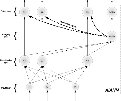
In the context of the immune system, recognition is accomplished through a lymphocyte, realizing that a cell in contact does not belong to the body when the number of bonds between the receptors and epitopes is larger than a threshold specific to each lymphocyte. In the AIANN, recognition is modeled by creating detectors for each class. Each of the detectors is implemented as the activation function of one of the neurons in the classification layer (or hidden layer) of the AIANN, as shown in Figure 2. The outputs of the detectors of each class are connected to a neuron in the output layer representing the class. If the number of detectors bonding with an input vector, i.e., recognizing the input as non-self and causing their corresponding neurons to fire, is larger than the threshold of the corresponding class output neuron, the output neuron fires indicating recognition of the input vector. The ambiguity node fires by generating an output equal to 1 if more than one class neuron declares the input vector belongs to the corresponding class, in which case the output layer neurons are ignored.

Fig 2.

Artificial Immune-Activated Neural Network (AIANN) Model.

AIANN-based MRI segmentation

The AIANN model was applied to the segmentation of brain 3D MRI data. The MR images are T1-weighted brain scans of 8-bit grayscale resolution, with the skull removed and the background voxels set exactly to 0s. In this context, the classes represent the tissue types of the different voxels in the 3D MRI brain data set, which are white matter, grey matter and CSF in the case of normal brain cases. In cases involving abnormal (disease affected) data that includes other tissues, e.g., multiple sclerosis lesions, additional classes corresponding to these tissues are added. Since the intensity distributions of white matter, gray matter, and CSF as well as other tissue of the brain may overlap, it would be insufficient to classify each voxel based on its grayscale intensity only. Instead, additional information about the grayscale intensities of the voxel’s neighbors is required to aid in the segmentation process. For that purpose, a n × n × n neighborhood centered at the voxel to be segmented (or classified according to its tissue type) is used to construct the input vector of features representing the voxel. The larger the value of n, the larger the size of the neighborhood affecting the voxel segmentation becomes. Considering the MRI fine resolution utilized for 3D acquisitions of 1-mm slice thickness, utilizing a large neighborhood renders the effect of distant (non-adjacent) voxels on the tissue type of a voxel more pronounced. For example, a value of n equal to 7 would result in voxels that are up to 5.2 mm away to affect the segmentation of a voxel, which is not conducive to efficient segmentation for most brain voxels based on the small anatomical structures including their position in the brain. In addition, the marginal gain for some brain voxels when utilizing a large neighborhood is offset by the additional time and complexity involved in a larger AIANN to handle such neighborhood. Consequently, the neighborhood utilized is based on a 3 × 3 × 3 volume surrounding the voxel, i.e., n is equal to 3, to account for local correlation of tissue types affected by adjacent voxels while avoiding the unnecessary influence of distant voxels. In other words, the neighborhood is composed of 27 voxels (voxel to be segmented and its 26 neighbors). The input vector of features representing the voxel is composed of the grayscale intensities of the 27 voxels and, hence, consists of 216 bits (27 voxels × 8 bits/voxel). The input vectors representing the voxels in the 3D MRI data set are presented to the AIANN as contiguous 216-bit binary strings and the classification results of the AIANN determine the tissue types of the voxels at the center of the corresponding neighborhoods.

PREPROCESSING

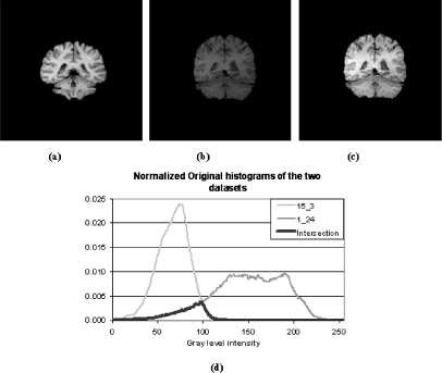
Since the segmentation is based on the grayscale intensities, it is sensitive to intensity level variations. Figure 3a–b demonstrates two slices from two different MRI data sets, obtained from the IBSR website, where the differences in brain data histogram are large as evident from Figure 3d.

Fig 3.

Intensity level correction: (a) sample slice from data set 1_24 (training data set); (b) and (c) sample slice from data set 15_3 before and after intensity correction, respectively; and (d) original histograms of 1_24 and 15_3 data sets.

If one data set is used for training, better histogram matching of the data set to be segmented and the training data set will lead to error reduction. Nonparametric histogram correction algorithms, e.g., histogram equalization and histogram stretching, do not guarantee good matching between a pair of histograms because there is no control on how the shape of the histogram will be modified. Moreover, histogram equalization moves voxels among bins in an effort to equalize the histogram distribution, which entails changing the intensity levels of a set of voxels irrelevant of what tissue those voxels originally represented, and what tissue will that final bin to which they are moved represent.

To address these concerns while matching against the training data set, contrast–brightness correction is first applied to maximize the intersection between the histograms of the two data sets based on the following:

29

where α is the contrast and β is the brightness.

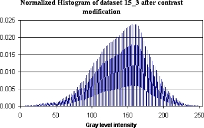
After modifying the brightness/contrast, empty bins appear in the brain volume histogram, an example of which is shown in Figure 4, depicting the histogram of data set 15_3 after contrast modification. Empty bins result in errors during histogram intersections if not corrected. To avoid those errors, the data set is filtered using a spatial anisotropic filter after the brightness/contrast correction. The 3D anisotropic filter that was previously discussed in the context of MRI conditioning⁷⁴ was used for that purpose. The parameters used for filtering were κ = 5 for 10 iterations.

Fig 4.

Histogram of data set 15_3 after contrast modification.

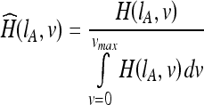
As the brain volumes vary from one MRI study to another, calculating the histogram intersections of large and small brain volumes is unreasonable. This necessitates that the histograms be normalized against the total number of voxels in their corresponding data sets.

Given two data sets I_A and I_B, the histogram of data set I_x at intensity level v is given by H(I_x, v). Let be the normalized histogram of data set I_x at intensity v, where the histogram is normalized against the total number of voxels in the brain as follows:

30

As maximizing the histogram intersection means maximizing the integral under the histogram intersection, then

31

where Ĥ(I_A, v) ∩ Ĥ(I_B, v) = min(Ĥ(I_A, v), Ĥ(I_B, v)).

If I_A is the data set used for training and I_B is the data set to be segmented, the brightness/contrast of I_B needs to be adjusted to maximize the intersection expressed in Eq. (31). Since the data set will be segmented after filtering with the anisotropic filter, the brightness/contrast adjustment needs to be maximized after applying the filter. However, the anisotropic filter depends on the spatial distribution of grayscale intensities of the voxels, which are used to calculate the filter gradients, and changing the brightness/contrast alters those gradients. Recursive adjustment of both brightness and contrast was evaluated through varying the brightness till is maximized and then varying the contrast till is maximized in a repetitive fashion. Results showed that the recursive adjustment method got trapped in local maxima and was not able to achieve better histogram intersection than 0.85.

As a result, searching for the values of α and β that maximize Eq. (31) after anisotropic filtering is carried out using genetic algorithms. The genetic algorithm has a population of chromosomes, each with one floating-point value for brightness and another for contrast. The population was initialized randomly with contrast values ranging from zero to three, and brightness values ranging from −64 to +64. The initialization ranges were empirically chosen to encompass a wide range of intensity variations. Mutation was carried out by multiplying each parameter in the new offspring by a random number from 0.999 to 1.001, which corresponds to a mutation of ±0.1%. The number of chromosomes in the population was 100, and the crossover ratio was 20%. Fitness of each individual chromosome was found by calculating the corresponding . The computation of the fitness involves applying the brightness/contrast to the data set and then filtering using the anisotropic filter with κ = 12 for one iteration only. Although the filter will be applied during segmentation with different parameters (κ = 5 and 10 iterations), setting those parameters during brightness/contrast adjustment dramatically increased the search time.

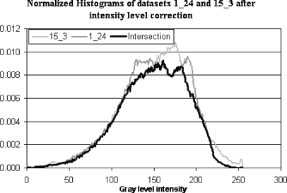
Figure 3c shows a slice from data set 15_3 after intensity level correction and Figure 5 demonstrates how the histogram intersection between the two data sets has changed.

Fig 5.

Histogram intersection of 1_24 and 15_3 after intensity levels correction.

EXPERIMENTAL RESULTS AND DISCUSSION

Segmentation of Real 3D MRI Brain Scans

A set of experiments was performed using real MRI brain scans to evaluate the segmentation performance of the AIANN model and compare with published techniques. This comparison is typically difficult to perform since most of the published techniques are applied to different MRI data sets that are not readily available. To perform the comparison, 20 real MRI brain data sets, which are publicly available on the Internet at the web site of the Center for Morphometric Analysis at Massachusetts General Hospital¹⁰⁷ were used. The 20 real MRI data sets are T1-weighted normal cases that were created, analyzed, and manually segmented as part of the Internet Brain Segmentation Repository (IBSR), an NIH-funded project. The IBSR data sets were selected for the comparison since they establish a common basis for the results of published techniques. The data sets also involve different levels of difficulty including low contrast scans, relatively smaller brain volumes, sudden intensity variations, and large spatial inhomogeneities, which enable the evaluation of the effect of signal-to-noise ratio, contrast-to-noise ratio, shape complexity and size variations on the segmentation results of the AIANN model. The results of the manual segmentation and five automated segmentation techniques are compared and published on the IBSR website using the Tanimoto coefficient T given by:

32

where |r| represents the number of voxels in region r, X and Y are the segmentations obtained for a tissue type using the manual and automated techniques, respectively. The Tanimoto coefficient is computed for both gray matter and white matter.

The training of the AIANN model was performed using all the slices of the 3D MRI data set 1_24. Then, segmentation of the other 19 data sets was performed using the trained model. Before segmenting each data set, the data set was filtered using the anisotropic filter with κ = 5 and for 10 iterations and then intensity level correction was applied. Table 1 shows the effect of intensity level correction on the histogram intersection of the 19 data sets with the training data set 1_24, where it is clear that some of the data sets had very low initial histogram intersection, and if segmentation was attempted without intensity level correction, worse results would have been obtained.

Table 1.

_int for Each Data Set Before and After Intensity Correction Against 1_24

Data set	Before Correction	After Correction
100_23	0.92	0.93
11_3	0.88	0.93
110_3	0.85	0.93
111_2	0.89	0.95
112_3	0.82	0.95
12_3	0.79	0.93
191_3	0.81	0.93
13_3	0.82	0.89
202_3	0.86	0.93
205_3	0.90	0.94
7_8	0.94	0.95
8_4	0.92	0.96
17_3	0.78	0.94
4_8	0.67	0.91
15_3	0.12	0.92
5_8	0.23	0.82
16_3	0.12	0.93
2_4	0.53	0.90
6_10	0.41	0.76

The AIANN segmentation results obtained, in terms of the Tanimoto coefficient, for the 19 MRI data sets are shown in Table 2 for two experiments. Experiment 1 involves obtaining the results without intensity correction to increase the histogram intersection with the training data set, whereas Experiment 2 includes the intensity correction. The results clearly demonstrate that intensity correction has a positive impact on the accuracy as the effect of contrast variation between the training data set and the data sets to be segmented was reduced.

Table 2.

AIANN Segmentation Results of IBSR Data in Terms of Tanimoto Coefficient

	Experiment #1 (Without Intensity Correction)		Experiment #2 (With Intensity Correction)
Data set	White	Gray	White	Gray
100_23	0.694	0.817	0.709	0.824
11_3	0.718	0.822	0.727	0.826
110_3	0.648	0.798	0.671	0.807
111_2	0.667	0.788	0.686	0.798
112_3	0.675	0.804	0.690	0.813
12_3	0.731	0.832	0.732	0.830
191_3	0.710	0.817	0.701	0.812
13_3	0.695	0.815	0.693	0.810
202_3	0.706	0.809	0.708	0.809
205_3	0.720	0.805	0.720	0.803
7_8	0.618	0.765	0.691	0.807
8_4	0.608	0.742	0.679	0.789
17_3	0.575	0.735	0.660	0.786
4_8	0.454	0.666	0.561	0.720
15_3	0.523	0.701	0.538	0.711
5_8	0.127	0.553	0.641	0.778
16_3	0.579	0.745	0.603	0.757
2_4	0.455	0.662	0.523	0.693
6_10	0.230	0.539	0.648	0.771
Average	0.586	0.748	0.662	0.787

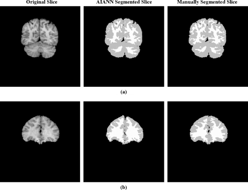
Then, the average Tanimoto coefficient obtained for the AIANN segmentation results of IBSR data sets was compared to results for the same data sets obtained using other techniques that were either registered at the IBSR website or recently reported using the same data sets⁹⁶ as shown in Table 3. It is clear from Table 3, which also includes the average Tanimoto coefficient between manual segmentations of different experts to represent the ground truth, that the segmentation results obtained using the AIANN model exhibited improvement in the objective measure of segmentation accuracy over published methods. In the case of the MPM-MAP method,⁹⁶ AIANN matched the performance for white matter while providing an advantage for gray matter. Figure 6 shows sample slices from the IBSR data sets along with the segmentation results of the AIANN model and the manually segmented results obtained by a human expert.

Table 3.

IBSR Results

White	Gray	Method
0.567	0.564	Adaptive MAP
0.562	0.558	Biased MAP
0.567	0.473	Fuzzy c-means
0.554	0.55	Maximum Aposteriori Probability (MAP)
0.551	0.535	Maximum-Likelihood
0.571	0.477	Tree-structure k-means
0.662	0.683	MPM-MAP 0
0.662	0.787	AIANN Model
0.832	0.876	Manual (4 brains averaged over 2 experts)

Fig 6.

Sample slices from IBSR data sets: (a) 100_23, (b) 11_3, and their AIANN and manual segmentations.

The sensitivity of the segmentation results of the AIANN model to the choice of training data set was evaluated by varying the training data set among 1_24, 100_23, 11_3, 12_3, and 13_3. An accelerated version of the training algorithm was utilized in this evaluation, which involves a reduced number of iterations to provide a rapid feedback about the effect of training data set. For each training data set, the trained AIANN model was used to segment the other 19 data sets after intensity correction to increase the intersection with the training data set and anisotropic filtering (κ = 5 and 10 iterations). The average Tanimoto coefficient for the other 19 data sets is shown in Table 4 for each training data set, where the variation is clearly limited, indicating that the effect of the training set on the AIANN segmentation results is relatively low.

Table 4.

AIANN Segmentation Results in Terms of Tanimoto Coefficient

Training Data Set	Average Tanimoto Coefficient for Other 19 Data Sets
	White	Gray
1_24	0.627	0.710
100_23	0.643	0.725
11_3	0.629	0.717
12_3	0.654	0.728
13_3	0.638	0.718

Segmentation of Simulated 3D MRI Data

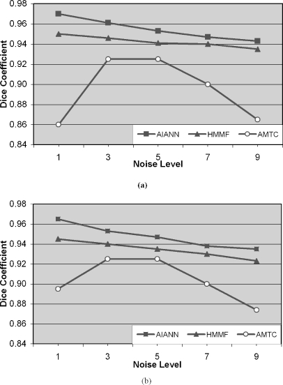
In this set of experiments, the AIANN model was evaluated for the segmentation of simulated MRI brain data sets generated using the BrainWeb MRI simulator,¹⁰⁸ which enables the creation of high-quality simulated MRI data sets from known anatomical models or ground truths for different levels of noise and spatial inhomogeneities. The MRI parameters utilized for the generation of the simulated MRI brain data sets are repetition time (TR) of 18 ms, echo time (TE) of 10 ms, and flip angle of 30°, which are identical to the parameters used in other published methods^97,98 to establish a common basis for comparison. The simulated MRI data sets were generated for varying levels of noise from 0% to 9% and no spatial inhomogeneities. The noiseless data set was used in the training of the AIANN model. Then, the trained AIANN model was applied to the segmentation of the other data sets after they were filtered using the anisotropic spatial filter for 10 iterations, with the κ parameter matched to the noise level (κ  = 1.5σ)¹¹⁰, where σ is the noise standard deviation that is estimated as percent noise multiplied by the mean of the white matter,¹⁰⁹ according to the definition of the percent noise in the BrainWeb simulated MRI data sets. For nonsimulated real MRI data, the anisotropic filter can be similarly applied with an estimate of noise standard deviation in any small region of uniform intensity in the background of real MRI data. The segmentation results of the AIANN model are shown in Figure 7 for white matter and gray matter in terms of the Dice coefficient, which was previously used to report the results of published methods for the same data and is defined as:

33

Fig 7.

Dice coefficient for BrainWeb-simulated MRI data sets: (a) White matter and (b) gray matter. Segmentation performed using the AIANN model, HMMF,⁹⁹ and ATCM¹⁰⁰.

Figure 7 also includes the reported results of published methods involving Hidden Markov Measure Field (HMMF)⁹⁷ and the Automated Tissue Classification Model (ATCM)⁹⁸ that use the same simulated data from BrainWeb for comparison. The results of the other two techniques, i.e., HMMF⁹⁷ and ATCM⁹⁸, were extracted from the respective publications that report the segmentation results of the same datasets generated through the BrainWeb MR simulator. In this manner, the comparison does include the parameters’ tuning of these techniques as reported in the respective publications^97,98. Comparison of the segmentation results in Figure 7 indicates that the presented AIANN model performed better than the automated tissue classification model⁹⁸ when applied to the BrainWeb simulated MRI data at all noise levels, with the advantage increasing at higher noise levels caused by the deterioration in performance of the ATCM. In comparison with the method based on HMMF⁹⁷, the AIANN performed marginally better than the HMMF based method at lower noise levels (1% and 5%), with the advantage decreasing for higher noise levels (7% and 9%). The decrease is caused by the reliance of the HMMF on prior probabilities, or a brain model/atlas, to influence the decision about individual brain voxels, which aids the segmentation process especially when higher levels of noise are affecting the MRI data. On the other hand, AIANN only relies on the anisotropic diffusion filter to reduce the effect of noise and as the noise level increases the potential for affecting regions of sharp intensity variations increases and the filter influence on such regions is inherently throttled based on the filter diffusion function that aims to preserve the sharp intensity variations, or edges, in the filtered image data.

CONCLUSION

In this paper, a novel MRI brain segmentation approach was presented based on an Artificial Immune-Activated Neural Network (AIANN) model. The AIANN model is based on an artificial immune activation function that conceptually mimics the biological adaptive immune system, which enables dynamic learning, storage of domain knowledge, and robust discrimination among classes. The classification process is modeled after the bonding process between receptors and epitopes in the immune system that is controlled through an energy function/measure to ensure accurate recognition. The artificial immunology fundamentals motivating the classification process in the AIANN model were presented. The AIANN model was detailed and the theoretical foundation establishing its characteristics was developed.

The contextual formulation of the problem of 3D MRI segmentation of the brain was developed and tackled using the AIANN model including the preprocessing steps involved in conditioning the 3D MRI data. The AIANN was evaluated based on the segmentation of both real MRI data, obtained from the MGH IBSR repository, and simulated MRI data generated from the BrainWeb MRI simulator. The comparison of the segmentation results obtained using the AIANN to those obtained using published methods has demonstrated its advantage for real MRI data and simulated MRI data, especially at low levels of noise. Future work will address the effect of including other MR contrasts, such as T2-weighted and FLAIR, on the segmentation results of the AIANN model, especially in the context of brain data for patients with brain lesions, e.g., due to Multiple Sclerosis (MS) or Stroke.

References

- 1.Jacobs MA, Knight RA, Soltanian-Zadeh H, Zheng ZG, Goussev AV, Peck DJ, Windham JP, Chopp M. Unsupervised segmentation of multiparameter MRI in experimental cerebral ischemia with comparison to T2, diffusion, and ADC MRI parameters and histopathological validation. J Magn Reson Imaging. 2000;11:425–437. doi: 10.1002/(SICI)1522-2586(200004)11:4<425::AID-JMRI11>3.0.CO;2-0. [DOI] [PubMed] [Google Scholar]
- 2.Burk DL, Means DC, Kennedy WH, Cooperstein LA, Herbert DL. Three-dimensional computed tomography of acetabula fractures. Radiology. 1985;155(1):183–186. doi: 10.1148/radiology.155.1.3975401. [DOI] [PubMed] [Google Scholar]
- 3.Hemm DC, David DJ, Herman GT. Three-dimensional reconstruction of craniofacial deformity using computed tomography. Neurosurgery. 1985;13(5):534–541. doi: 10.1227/00006123-198311000-00009. [DOI] [PubMed] [Google Scholar]
- 4.Tessier PL, Hemmy DC. CT of dry skulls with craniofacial deformities: Accuracy of three-dimensional reconstruction. Radiology. 1985;157(1):113–116. doi: 10.1148/radiology.157.1.3929326. [DOI] [PubMed] [Google Scholar]
- 5.Farrell EJ, Zapulla R. Color 3D imaging of normal and pathologic intracranial structures. IEEE Comput Graph Appl. 1984;4(9):5–7. doi: 10.1109/MCG.1984.275989. [DOI] [Google Scholar]
- 6.Barillot C, Giband B, Scarabin J, Coatreux J. 3D Reconstruction of cerebral blood vessels. IEEE Comput Graph Appl. 1984;5(12):13–19. doi: 10.1109/MCG.1985.276258. [DOI] [Google Scholar]
- 7.Hale JD, Valk PE, Watts JC, Kauffman L, Crooks LE, Higgins CB, Decominck F. MR imaging of blood vessels using three-dimensional reconstruction methodology. Radiology. 1985;157(3):727–733. doi: 10.1148/radiology.157.3.4059560. [DOI] [PubMed] [Google Scholar]
- 8.Greenberg D, Sunguroff A. Computer generated images for medical application. Comput Graph. 1978;12(3):196–202. doi: 10.1145/965139.807390. [DOI] [Google Scholar]
- 9.Cook L T, Cook PN, Lee KR, Batnizley S, Wong BYS, Fritz SL, Ophir J, Dwyer SJ, Bigongiari LR, Templeton AW. A three-dimensional display system for diagnostic imaging applications. IEEE Comput Graph Appl. 1983;3(5):13–19. doi: 10.1109/MCG.1983.263180. [DOI] [Google Scholar]
- 10.Udupa JK, Bloch RH. Application of computerized tomography to radiation therapy and surgical planning. Proc IEEE. 1983;71(3):351–372. doi: 10.1109/PROC.1983.12599. [DOI] [Google Scholar]
- 11.Brewster LJ, Trivedi SS, Tuy HK, Udupa JK. Interactive surgical planning. IEEE Comput Graph Appl. 1984;4(3):31–40. doi: 10.1109/MCG.1984.276061. [DOI] [Google Scholar]
- 12.Totty WG, Vannier MW. Three-dimensional CT reconstruction images for craniofacial surgery planning and evaluation. Radiology. 1984;150(1):179–184. doi: 10.1148/radiology.150.1.6689758. [DOI] [PubMed] [Google Scholar]
- 13.Shareef N, Wang DL, Yagel R. Segmentation of medical images using LEGION. IEEE Trans Med Imaging. 1999;18(1):74–91. doi: 10.1109/42.750259. [DOI] [PubMed] [Google Scholar]
- 14.Thirion J-P, Declerck J, Subsol G, Ayache N: Automatic retrieval of anatomical structures in 3d medical images. Tech Rep 2458, INRIA, 1995
- 15.Warfield SK, Nabavi A, Butz T, Tuncali K, Silverman SG, Black P, Jolesz FA, Kikinis R: Intraoperative segmentation and nonrigid registration for image guided therapy. MICCAI 2000: Third International Conference on Medical Robotics, Imaging And Computer Assisted Surgery, 2000, pp. 176–185
- 16.Jernigan ME, Alirezaie J, Nahimias C. Automatic segmentation of cerebral MR images using artificial neural networks. IEEE Trans Nucl Sci. 1998;45(4):2174–2182. doi: 10.1109/23.708336. [DOI] [Google Scholar]
- 17.Atkins MS, Tauber Z, Drew MS. Towards automatic segmentation of conspicuous MS lesions in PD/T2 MR images. Proceedings of the SPIE-Medical Imaging Conference, 2000, pp. 800–809
- 18.Kaufhold J, Schneider M, Karl WC, Willsky A: MR image segmentation and data fusion using a statistical approach. International Conference on Image Processing (ICIP ’97), Oct 1997
- 19.Nabavi A, Black PM, Jolesz FA, Kaus MR, Warfield SK, Kikinis R. Automated segmentation of MRI of brain tumors. Radiology. 2001;218(2):586–591. doi: 10.1148/radiology.218.2.r01fe44586. [DOI] [PubMed] [Google Scholar]
- 20.Jolesz FA, Warfield SK, Kaus M, Kikinis R. Adaptive, template moderated, spatially varying statistical classification. Med Image Anal. 2000;4(1):43–55. doi: 10.1016/S1361-8415(00)00003-7. [DOI] [PubMed] [Google Scholar]
- 21.Web link: http://bishopw.loni.ucla.edu/AIR3/
- 22.Web link: http://stp.wustl.edu/caret.html
- 23.Mui JK, Fu KS: A survey on image segmentation. Pattern Recogn 13:3–16, 1981.
- 24.Ozkan M, Sprenkels HG, Dawant BM: Multi-spectral magnetic resonance image segmentation using neural networks. Proceedings 1990 International Joint Conference on Neural Networks (IJCNN ’90), Jun 1990, pp. 429–434
- 25.Takefuji Y, Amartur S, Piraaino D: Optimization of neural networks for the segmentation of magnetic resonance images. IEEE Trans Med Imaging, 11(2):215–220, 1992 [DOI] [PubMed]
- 26.Rajapakee J, Acharya R: Medical image segmentation with MARA. Proceedings 1990 International Joint Conference on Neural Netwotks (IJCNN ’90), Jun 1990, pp. 965–972
- 27.Katz WT, Merickel MB: Translation-invariant aorta segmentation from magnetic resonance images. Proceedings 1989 International Joint Conference on Neural Networks (IJCNN ’89), Jun 1989, pp. 327–333
- 28.Chen C, Tsao EC, Lin W: Medical image segmentation by a constraint satisfaction neural network. IEEE Trans Nucl Sci, 38(2):678–686, 1991
- 29.GoldBerg M, Beaulieu M: Hierarchy in picture segmentation: A stepwise optimization approach. IEEE Trans Pattern Anal Mach Intell, 11(2):150–163, February 1989
- 30.Gonzalez R, Perez A: An iterative thresholding algorithm for image segmentation. IEEE Trans Pattern Anal Mach Intell, 9(6):742–751, November 1987 [DOI] [PubMed]
- 31.Sklansky J, Gutfinger D. Tissue identification in MR images by adaptive cluster analysis. SPIE Image Processing. 1991;1445:288–298. [Google Scholar]
- 32.Amamoto DY, Kasturi R, Mamourian A: Tissue-type discrimination in magnetic resonance images. Proceedings of the 10th International Conference on Pattern Recognition, June 1990, pp. 603–607
- 33.Unser M, Eden M: Multiresolution feature extraction and selection for texture segmentation. IEEE Trans Pattern Anal Mach Intell, 11(7):717–728, July 1989
- 34.Saeed N, Hajnal JV, Oatridge A: Automated brain segmentation from single slice, multislice, or whole-volume MR scans using prior knowledge. J Comput Assist Tomogr, 21(2):192–201, 1997 [DOI] [PubMed]
- 35.Poon CS, Braun M: Image segmentation by a deformable contour model incorporating region analysis. Phys Med Biol, 42:1833–1841, 1997 [DOI] [PubMed]
- 36.Goldszal AF, Davatzikos C, Pham DL, Yan MX, Bryan RN, Resnick SM. An image-processing system for qualitative and quantitative volumetric analysis of brain images. J Comput Assist Tomogr. 1998;22:827–837. doi: 10.1097/00004728-199809000-00030. [DOI] [PubMed] [Google Scholar]
- 37.Talairach J, Tournoux P. Co-Planar Stereotaxic Atlas of the Human Brain. New York: Thieme Medical; 1988. [Google Scholar]
- 38.Resnick SM, Goldszal AF, Davatzikos C, Golski S, Kraut MA, Metter EJ, Bryan RN, Zonderman AB. One-year age changes in MRI brain volumes in older adults. Cereb Cortex. 2000;10:464–472. doi: 10.1093/cercor/10.5.464. [DOI] [PubMed] [Google Scholar]
- 39.Watson C, Jack CR, Jr, Cendes F. Volumetric magnetic resonance imaging. Clinical applications and contributions to the understanding of temporal lobe epilepsy. Arch Neurol. 1997;54:1521–1531. doi: 10.1001/archneur.1997.00550240071015. [DOI] [PubMed] [Google Scholar]
- 40.Jack CR, Jr, Petersen RC, Xu YC, O’Brien PC, Smith GE, Ivnik RJ, Boeve BF, Waring SC, Tangalos EG, Kokmen E. Prediction of AD with MRI-based hippocampal volume in mild cognitive impairment. Neurology. 1999;52:1397–1403. doi: 10.1212/wnl.52.7.1397. [DOI] [PMC free article] [PubMed] [Google Scholar]
- 41.Udupa JK, Nyul LG, Ge Y, Grossman RI. Multiprotocol MR image segmentation in multiple sclerosis: Experience with over 1,000 studies. Acad Radiol. 2001;8:1116–1126. doi: 10.1016/S1076-6332(03)80723-7. [DOI] [PubMed] [Google Scholar]
- 42.Mohamed FB, Vinitski S, Gonzalez CF, Faro SH, Lublin FA, Knobler R, Gutierrez JE. Increased differentiation of intracranial white matter lesions by multispectral 3D-tissue segmentation: Preliminary results. Magn Reson Imaging. 2001;19:207–218. doi: 10.1016/S0730-725X(01)00291-0. [DOI] [PubMed] [Google Scholar]
- 43.Alfano B, Brunetti A, Larobina M, Quarantelli M, Tedeschi E, Ciarmiello A, Covelli EM, Salvatore M. Automated segmentation and measurement of global white matter lesion volume in patients with multiple sclerosis. J Magn Reson Imaging. 2000;12:799–807. doi: 10.1002/1522-2586(200012)12:6<799::AID-JMRI2>3.0.CO;2-#. [DOI] [PubMed] [Google Scholar]
- 44.Catalaa I, Grossman RI, Kolson DL, Udupa JK, Nyul LG, Wei L, Zhang X, Polansky M, Mannon LJ, McGowan JC. Multiple sclerosis: Magnetization transfer histogram analysis of segmented normal-appearing white matter. Radiology. 2000;216:351–355. doi: 10.1148/radiology.216.2.r00au16351. [DOI] [PubMed] [Google Scholar]
- 45.Catalaa I, Fulton JC, Zhang X, Udupa JK, Kolson D, Grossman M, Wei L, McGowan JC, Polansky M, Grossman RI. MR imaging quantitation of gray matter involvement in multiple sclerosis and its correlation with disability measures and neurocognitive testing. AJNR Am J Neuroradiol. 1999;20:1613–1618. [PMC free article] [PubMed] [Google Scholar]
- 46.Sailer M, Losseff NA, Wang L, Gawne-Cain ML, Thompson AJ, Miller DH. T1 lesion load and cerebral atrophy as a marker for clinical progression in patients with multiple sclerosis. A prospective 18 months follow-up study. Eur J Neurol. 2001;8:37–42. doi: 10.1046/j.1468-1331.2001.00147.x. [DOI] [PubMed] [Google Scholar]
- 47.Ellis CM, Suckling J, Amaro E, Jr, Bullmore ET, Simmons A, Williams SC, Leigh PN. Volumetric analysis reveals corticospinal tract degeneration and extramotor involvement in ALS. Neurology. 2001;57:1571–1578. doi: 10.1212/wnl.57.9.1571. [DOI] [PubMed] [Google Scholar]
- 48.Nowinski WL, Bryan RN, Ragahavan R. The electronic clinical brain atlas on CD-ROM. New York: Thieme Medical; 1997. [Google Scholar]
- 49.Wiedermann D, Schuff N, Matson GB, Soher BJ, Du AT, Maudsley AA, Weiner MW. Short echo time multislice proton magnetic resonance spectroscopic imaging in human brain: Metabolite distributions and reliability. Magn Reson Imaging. 2001;19:1073–1080. doi: 10.1016/S0730-725X(01)00441-6. [DOI] [PubMed] [Google Scholar]
- 50.Lundbom N, Barnett A, Bonavita S, Patronas N, Rajapakse J, Tedeschi, Chiro G. MR image segmentation and tissue metabolite contrast in 1H spectroscopic imaging of normal and aging brain. Magn Reson Med. 1999;41:841–845. doi: 10.1002/(SICI)1522-2594(199904)41:4<841::AID-MRM25>3.0.CO;2-T. [DOI] [PubMed] [Google Scholar]
- 51.MacKay S, Ezekiel F, Sclafani V, Meyerhoff DJ, Gerson J, Norman D, Fein G, Weiner MW. Alzheimer disease and subcortical ischemic vascular dementia: Evaluation by combining MR imaging segmentation and H-1 MR spectroscopic imaging. Radiology. 1996;198:537–545. doi: 10.1148/radiology.198.2.8596863. [DOI] [PMC free article] [PubMed] [Google Scholar]
- 52.Tanna NK, Kohn MI, Horwich DN, Jolles PR, Zimmerman RA, Alves WM, Alavi A. Analysis of brain and cerebrospinal fluid volumes with MR imaging: Impact on PET data correction for atrophy. Part II. Aging and Alzheimer dementia. Radiology. 1991;178:123–130. doi: 10.1148/radiology.178.1.1984290. [DOI] [PubMed] [Google Scholar]
- 53.Bowen BC, Pattany PM, Bradley WG, Murdoch JB, Rotta F, Younis AA, Duncan RC, Quencer RM. MR imaging and localized proton spectroscopy of the precentral gyrus in amyotrophic lateral sclerosis. AJNR Am J Neuroradiol. 2000;21:647–658. [PMC free article] [PubMed] [Google Scholar]
- 54.Bowen BC, DePrima S, Pattany PM, Marcillo A, Madsen P, Quencer RM. MR angiography of normal intradural vessels of the thoracolumbar spine. AJNR Am J Neuroradiol. 1996;17:483–494. [PMC free article] [PubMed] [Google Scholar]
- 55.Bowen BC. MR angiography of spinal vascular disease: What about normal vessels? AJNR Am J Neuroradiol. 1999;20:1773–1774. [PMC free article] [PubMed] [Google Scholar]
- 56.Flasque N, Desvignes M, Constans JM, Revenu M. Acquisition, segmentation and tracking of the cerebral vascular tree on 3D magnetic resonance angiography images. Med Image Anal. 2001;5:173–183. doi: 10.1016/S1361-8415(01)00038-X. [DOI] [PubMed] [Google Scholar]
- 57.Stefancik RM, Sonka M. Highly automated segmentation of arterial and venous trees from three-dimensional magnetic resonance angiography (MRA) Int J Card Imaging. 2001;17:37–47. doi: 10.1023/A:1010656618835. [DOI] [PubMed] [Google Scholar]
- 58.Martland D: Auto-associative pattern storage using synchronous Boolean network, Proceedings of the First IEEE Conference on Neural Networks, San Deigo, vol. III, 1987, pp. 355–366
- 59.Martinez T: “Models of parallel adaptive logic,” Proceedings of 1987 Systems, Man and Cybernetics Conference Oct 1987, pp. 290–296
- 60.Sen S: Genetic learning of logic functions. Proceedings of the Artificial Neural Networks in Engineering Conference, November 1991, pp. 83–88
- 61.Papadakis INM: PACNET: A pattern classification neural network, Proceedings 1991 International Joint Conference on Neural Networks, July 1991, pp. 17–22
- 62.Shin Y and Ghosh J: Realization of boolean functions using binary pi-sigma networks. Proceedings of Artificial neural Networks in Engineering conference, Nov 1991, pp. 205–210
- 63.Macek T, Morgan G, Austin J: A transputer implementation of the ADAM neural network. World Transputer Congress’95, Harrogate, UK, 1995
- 64.Hussain B, Kabuka MR. A novel feature recognition neural network and its application to character recognition. IEEE Trans Pattern Anal Mach Intell. 1994;16(1):99–106. doi: 10.1109/34.273711. [DOI] [Google Scholar]
- 65.Hussain B and Kabuka MR: A high performance recognition neural network for character recognition. Proceedings of Second International Conference on Automation, Robotics and Computer Vision (ICARCV), Singapore, 1992
- 66.Bhide S, Gazula S, Guerrero V, Shebert G and Kabuka M: An ASIC implementation of a user configurable Boolean Neural Network. Proceedings of World Congress on Neural Networks, WCNN’93, Vol. IV, July 1993, pp 239—244
- 67.Gazula S and Kabuka MR: Real-time implementation of supervised classifiers using Boolean Neural Networks. In C.H. Dagli et al, Eds. Proceedings of Artificial Neural Networks in Engineering, Nov. 1992
- 68.Bhide S, John N, Kabuka MR. A Boolean neural network approach for the traveling salesman problem. IEEE Trans Comput. 1993;42(10):1271–1278. doi: 10.1109/12.257714. [DOI] [Google Scholar]
- 69.John N, Bhide S, Kabuka MR: A real-time solution for the traveling salesman problem. IEEE International Conference on Neural Networks, San Francisco, California, pp. 1096–1103, 1993
- 70.Gazula S, Kabuka MR. Design of supervised classifiers using Boolean neural networks. IEEE Trans Pattern Anal Mach Intell. 1995;117(2):1239–1246. doi: 10.1109/34.476519. [DOI] [Google Scholar]
- 71.Gazula S, Kabuka MR: Real-time hierarchical clustering using Boolean neural network. Artificial Neural Networks in Engineering, St. Loius, MO, 1993
- 72.Hussain B, Kabuka MR. Neural network transformation of arbitrary Boolean functions. SPIE. 1992;1766:355–367. doi: 10.1117/12.130842. [DOI] [Google Scholar]
- 73.Li X, Bhide S, Kabuka M. Labeling of MR brain images using Boolean neural network. IEEE Trans Med Imaging. 1996;15(5):628–638. doi: 10.1109/42.538940. [DOI] [PubMed] [Google Scholar]
- 74.John N, Kabuka M, Ibrahim M. Multivariate statistical model for 3D image segmentation with application to medical images. J Digit Imaging. 2004;17(4):365–377. doi: 10.1007/s10278-003-1664-9. [DOI] [PMC free article] [PubMed] [Google Scholar]
- 75.Hajela P, Lee J: Constrained genetic search via schema adaptation: An immune network solution. Struct Multidiscipl Optim 12(1):11–15, 1996
- 76.De Castro LN, Von Zuben FJ: Learning and optimization using the clonal selection principle. IEEE Trans Evol Comput 6(3):239–251, 2002
- 77.Hart E, Ross PM: An immune system approach to scheduling in changing environments, GECCO-99: Proceedings of the Genetic and Evolutionary Computation Conference, 1999 pp. 1559–1565
- 78.Hart E, Ross PM: The evolution and analysis of a potential antibody library for use in job-shop scheduling. In Corne D, Dorigo M, and Glover F, Eds. New Ideas in Optimisation, 1999 pp. 185–202
- 79.De Castro LN, Von Zuben FJ: An immunological approach to initialize feedforward neural network weights. Proceedings of International Conference on Artificial Neural Networks and Genetic Algorithms (ICANNGA 2001), 2001 pp. 126–129
- 80.De Castro LN, Von Zuben FJ: An immunological approach to initialize centers of radial basis function neural networks. Proceedings of CBRN 2001 (Congresso Brasileiro de Redes Neurais), 2001 pp. 79–84
- 81.De Castro LN, Von Zuben FJ, de Deus GA: The construction of a Boolean competitive neural network using ideas from immunology. Neurocomputing 50:51–58, 2003
- 82.Abbattista F, Di Gioia G, Di Santo G, Fanelli AM: An associative memory based on the immune networks, IEEE International Conf. on Neural Networks, 1996, pp. 519–523
- 83.De Castro LN, Von Zuben FJ: An evolutionary immune network for data clustering, Proceedings of IEEE SBRN, 2000 pp. 84–89
- 84.De Castro LN, Von Zuben FJ: AINet: An artificial immune network for data analysis. In: Abbas HA, Sarker RA, Newton CS Eds. Data Mining: A Heuristic Approach, Chapter III. USA: Idea Group Publishing, 2001, pp. 231–259
- 85.De Castro LN, Von Zuben FJ: Artificial immune systems: Part II–A survey of applications, Technical Report DCA-RT 02/00, Department of Computer Engineering and Industrial Automation, State University of Campinas, SP, Brazil, 2000
- 86.Somayaji FJ, Forrest S, Hofmeyer SA. Computer immunology. Commun ACM. 1997;40(10):88–96. doi: 10.1145/262793.262811. [DOI] [Google Scholar]
- 87.Forrest S, Hofmeyr SA: Immunity by design: An artificial immune system. Proceedings of the Genetic and Evolutionary Computation Conference (GECCO), Morgan-Kaufmann, San Francisco, CA, 1999, pp. 1289–1296
- 88.Ibrahim MO, Shahein HI: Modeling and generation of detectors in artificial immune based intrusion detection systems. Proceedings of 3rd Scientific Conference on Computers and Applications (SCCA’ 2000), Jordan, Feb 2001
- 89.Grabowski TJ, Frank RJ, Szumski NR, Brown CK, Damasio H. Validation of partial tissue segmentation of single-channel magnetic resonance images of the brain. NeuroImage. 2000;12:640–656. doi: 10.1006/nimg.2000.0649. [DOI] [PubMed] [Google Scholar]
- 90.Kovacevic N, Lobaugh NJ, Bronskill MJ, Levine B, Feinstein A, Black SE. A robust method for extraction and automatic segmentation of brain images. NeuroImage. 2002;17:1087–1100. doi: 10.1006/nimg.2002.1221. [DOI] [PubMed] [Google Scholar]
- 91.Rajapakse JC, Giedd JN, DeCarli C, Snell JW, McLaughlin A, Vauss YC, Krain AL, Hamburger S, Rapoport JL. A technique for single-channel MR brain tissue segmentation: Application to a pediatric sample. Magn Reson Imaging. 1996;14:1053–1065. doi: 10.1016/S0730-725X(96)00113-0. [DOI] [PubMed] [Google Scholar]
- 92.Schnack HG, Hulshoff Pol HE, Baare WF, Staal WG, Viergever MA, Kahn RS. Automated separation of gray and white matter from MR images of the human brain. NeuroImage. 2001;13:23–237. doi: 10.1016/S1053-8119(01)91366-7. [DOI] [PubMed] [Google Scholar]
- 93.Ruan S, Jaggi C, Xue J, Fadili J, Bloyet D. Brain tissue classification of magnetic resonance images using partial volume modeling. IEEE Trans Med Imaging. 2000;19:1179–1187. doi: 10.1109/42.897810. [DOI] [PubMed] [Google Scholar]
- 94.Held K, Kops ER, Krause BJ, Wells WM, Kikinis R, Muller-Gartner HW. Markov random field segmentation of brain MR images. IEEE Trans Med Imaging. 1997;16:878–886. doi: 10.1109/42.650883. [DOI] [PubMed] [Google Scholar]
- 95.Rajapakse JC, Giedd JN, Rapoport JL. Statistical approach to segmentation of single-channel cerebral MR images. IEEE Trans Med Imaging. 1997;16:176–186. doi: 10.1109/42.563663. [DOI] [PubMed] [Google Scholar]
- 96.Marroquin JL, Vemuri BC, Botello S, Calderon F, Fernandez-Bouzas A. An accurate and efficient bayesian method for automatic segmentation of brain MRI. IEEE Trans Med Imaging. 2002;21(8):934–945. doi: 10.1109/TMI.2002.803119. [DOI] [PubMed] [Google Scholar]
- 97.Marroquin JL, Santana EA, Botello S. Hidden markov measure field models for image segmentation. IEEE Trans Pattern Anal Mach Intell. 2003;25(11):1380–1387. doi: 10.1109/TPAMI.2003.1240112. [DOI] [Google Scholar]
- 98.Leemput K, Maes F, Vandermeulen D, Suetens P. Automated model-based tissue classification of MR images of the brain. IEEE Trans Med Imaging. 1999;18:897–908. doi: 10.1109/42.811270. [DOI] [PubMed] [Google Scholar]
- 99.Leemput K, Maes F, Vandermeulen D, Suetens P. A statistical framework for partial volume segmentation. Lect Notes Comput Sci. 2001;2208:204–212. doi: 10.1007/3-540-45468-3_25. [DOI] [Google Scholar]
- 100.Leemput K, Maes F, Vandermeulen D, Suetens P. A unifying framework for partial volume segmentation of brain MR images. IEEE Trans Med Imaging. 2003;22(1):105–119. doi: 10.1109/TMI.2002.806587. [DOI] [PubMed] [Google Scholar]
- 101.Forrest S, Oprea M: How the immune system generates diversity: Pathogen space coverage with random and evolved antibody libraries. Proc. Genetic Evolutionary Computation Conf. (GECCO), July 1999, pp. 1651–1656
- 102.Hofmeyr SA: An immunological model for distributed detection and its application to computer security. Ph.D. Dissertation, University of New Mexico, 1999
- 103.Ashburner J, Friston KJ. Voxel-based morphometry—The methods. NeuroImage. 2000;11:805–821. doi: 10.1006/nimg.2000.0582. [DOI] [PubMed] [Google Scholar]
- 104.Watkins A, Boggess L. A resource limited artificial immune classifier. Proceedings of the 2002 Congress on Evolutionary Computation (CEC ‘02), 12–17 May 2002, vol. 2, pp. 926–931
- 105.Watkins A, Boggess L: A new classifier based on resource limited artificial immune systems. Proceedings of the 2002 Congress on Evolutionary Computation (CEC ‘02) 12–17 May 2002, vol. 2, pp. 1546–1551,
- 106.Lei Wang, Licheng Jiao: An immune neural network used for classification. Proc IEEE Int Conference on Data Mining (ICDM 2001), San Jose, CA, 29 Nov–2 Dec, 2001, pp. 657–658
- 107.Internet Brain Segmentation Repository (IBSR). Technical Report, Mass. General Hospital, Center for Morphometric Analysis, 2000. [Online] Available: http://neuro-www.mgh.harvard.edu/cma/ibsr.
- 108.Cocosco CA, Kollokian V, Kwan RK, Evans AC: BrainWeb: Online interface to a 3D MRI simulated brain database. NeuroImage 5(4), parts 2/4, S245, 1997
- 109.Collins DL, Zijdenbos AP, Kollokian V, Sled JG, Kabani NJ, Holmes CJ, Evans AC: Design and construction of a realistic digital brain phantom. IEEE Trans Med Imaging 17(3):463–468, June 1998 [DOI] [PubMed]
- 110.Zijdenbos AP, Dawant BM, Margolin RA, Palmer AC. Morphometric analysis of white matter lesions in MR images: Method and validation. IEEE Trans Med Imaging. 1994;13(4):716–724. doi: 10.1109/42.363096. [DOI] [PubMed] [Google Scholar]
- 111.Juang B, Chou W, Lee C. Minimum classification error rate methods for speech recognition. IEEE Trans Speech Audio Processing. 1997;5(3):257–265. doi: 10.1109/89.568732. [DOI] [Google Scholar]
- 112.Katagari S, Juang B, Lee C. Pattern recognition using a family of design algorithms based upon the generalized probabilisitic descent method. Proc IEEE. 1998;86(11):2345–2373. doi: 10.1109/5.726793. [DOI] [Google Scholar]