Part 1. Automated Change Detection and Characterization in Serial MR Studies of Brain-Tumor Patients

Abstract

The goal of this study was to create an algorithm which would quantitatively compare serial magnetic resonance imaging studies of brain-tumor patients. A novel algorithm and a standard classify–subtract algorithm were constructed. The ability of both algorithms to detect and characterize changes was compared using a series of digital phantoms. The novel algorithm achieved a mean sensitivity of 0.87 (compared with 0.59 for classify–subtract) and a mean specificity of 0.98 (compared with 0.92 for classify–subtract) with regard to identification of voxels as changing or unchanging and classification of voxels into types of change. The novel algorithm achieved perfect specificity in seven of the nine experiments. The novel algorithm was additionally applied to a short series of clinical cases, where it was shown to identify visually subtle changes. Automated change detection and characterization could facilitate objective review and understanding of serial magnetic resonance imaging studies in brain-tumor patients.

INTRODUCTION

Comparison of serial MR studies of brain-tumor patients is a common clinical task whose difficulty is widely recognized. This difficulty results from the method of data presentation, which is not well suited to our cognitive capabilities,^1,2 as well as factors related to image acquisition and processing.³ The issue of change detection has been one of interest in fields of image processing beyond those of medical imaging.⁴ Within medical imaging, various methods have been used to effect serial comparisons, including manual inspection, measurement sampling (such as maximum diameter methods),^5–11 volumetrics,^12–14 warping,^15–18 and temporal analysis.^19,20 It is widely recognized that each of these methods possesses both merits and shortcomings; a thorough description of these considerations may be found elsewhere.³ We hypothesized that a system could be developed to detect and characterize changes in serial magnetic resonance (MR) studies of brain-tumor patients. It was desired that this system be highly automated, produce quantitative metrics, and be resistant to acquisition-related changes.

METHODS

Image Acquisition

After IRB approval, we obtained informed consent from 65 patients who had a prior biopsy-confirmed diagnosis of glioma. Images were acquired at baseline and for at least one follow-up using T1, T1 Post-Gd, and FLAIR sequences with acquisition parameters: T1: TR between 450 and 600, TE min full; FLAIR: TR 11,000, TE 144ef; FOV 20–22 cm; pixel size 0.86–0.93 mm in X and Y, and 3 mm in Z, with an interslice gap of 0 mm. While the algorithm is not limited to these particular pulse sequences and acquisition parameters, these were the datasets used for this study.

Preparation of Cases

The preprocessing steps used in the present work are shown in Figure 1. The first step consisted of inhomogeneity correction using the N3 software package.²¹ In the second step, registration of serial examination pairs, both within a particular exam, and between serial exams, was performed so that a common spatial framework was established. In this study, we used the mutual information registration application of the ITK software package²² (http://www.itk.org) to register all images to the T1-weighted image from the baseline acquisition. After this, a brain mask was defined manually, separating the brain and cerebrospinal fluid (CSF) from all nonbrain tissues. In this study, this was performed using the Image Edit component of the Analyze software package.²³ Finally, samples of normal-appearing white matter (NAWM) were defined also using the Image Edit component of the Analyze software package. For consistency, these samples were specified within the frontal lobes and anterior corpus callosum, unless this was impossible due to pathology. In practice, no specific number of voxels was required although 100 voxels served as a useful target.

Fig 1.

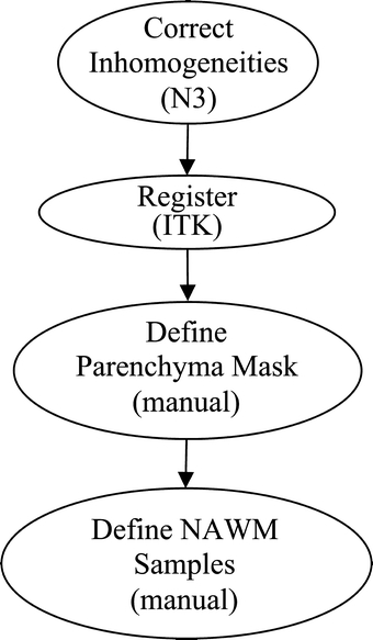
Preprocessing.

Change Detection Algorithm

The change detection algorithm may be described as a series of processing steps (Fig. 2). In the first step, sample points for all tissues of interest are generated using the samples of NAWM provided by the user, in conjunction with anatomical knowledge and knowledge of relationships between tissue intensities for each pulse sequence. This process of automatically locating sample points is performed for: CSF and normal gray matter. The algorithm additionally either locates or synthetically creates sample points for three pathological “tissues”: nonenhancing T2 abnormality (NETTA), enhancing tissue, and necrosis. It should be noted that while there are often no “pure” pathologic tissues, within this article, the most extreme examples of these pathological states (i.e., enhancing lesion with the brightest possible enhancement, NETTA with the brightest possible FLAIR intensity, and necrosis with the lowest possible T1 intensity) were treated as if they are in fact distinct tissue types.

Fig 2.

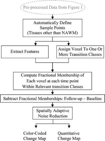
Change detection algorithm.

In order to either locate or create samples for each of the normal and pathological tissues, the algorithm first predicts the multispectral intensities of their centroids based upon the manually defined NAWM intensities using a mathematical model which we have developed, which consists of a set of linear functions of NAWM intensity. Using these predicted intensities, in conjunction with anatomical knowledge, the algorithm attempts to locate the samples of each of these tissues within each exam. If the algorithm is able to locate samples for a given tissue, the centroid intensity of the located samples is calculated. If the algorithm is unable to locate sample voxels (i.e., when a certain exam does not have a particular pathologic tissue type), synthetic sample points are generated based upon the intensities predicted above. In all cases (i.e., whether the centroid is calculated from real samples or predicted via the model), the noise characteristics are drawn from those of the manually provided white-matter samples. The reason for always using noise characteristics drawn from the manually defined NAWM samples is that for many tissues (particularly pathological tissues), the number of samples available is not adequate to compute a reasonable estimate of the noise characteristics even when a satisfactory estimate of the centroid intensity is possible.

The change detection algorithm makes the approximation that voxels contain mixtures of at most two tissues. In this article, these mixtures will be referred to as “tissue pairs”, and it is assumed that changes observed in a voxel between examinations occur between the pairs of tissues. In the general case, dual-tissue classes may consist of any pair of tissues which may be observed to be partial-volumed or mixed within a voxel. In the present study, we were interested only in dual-tissue classes which were relevant to white-matter changes due to primary brain tumors. The dual-tissue classes relevant to the algorithm were thus: NAWM and NETTA, NAWM and enhancement, NETTA and enhancement, enhancement and necrosis, and NETTA and necrosis. In a scatterplot describing the feature space, lines can be drawn connecting the centroids of the tissues in each of the above pairs. In this article, these lines will be called partial membership lines; an example of a partial membership line is shown in Figure 3a; for the tissue pair of NAWM and NETTA, i.e., as white matter, which was previously normal-appearing, acquires NETTA, we assumed in this study that the voxel’s multispectral intensity would follow this line in feature space (offset by noise). This is an approximation which proved adequate for the purposes of this study.

Fig 3.

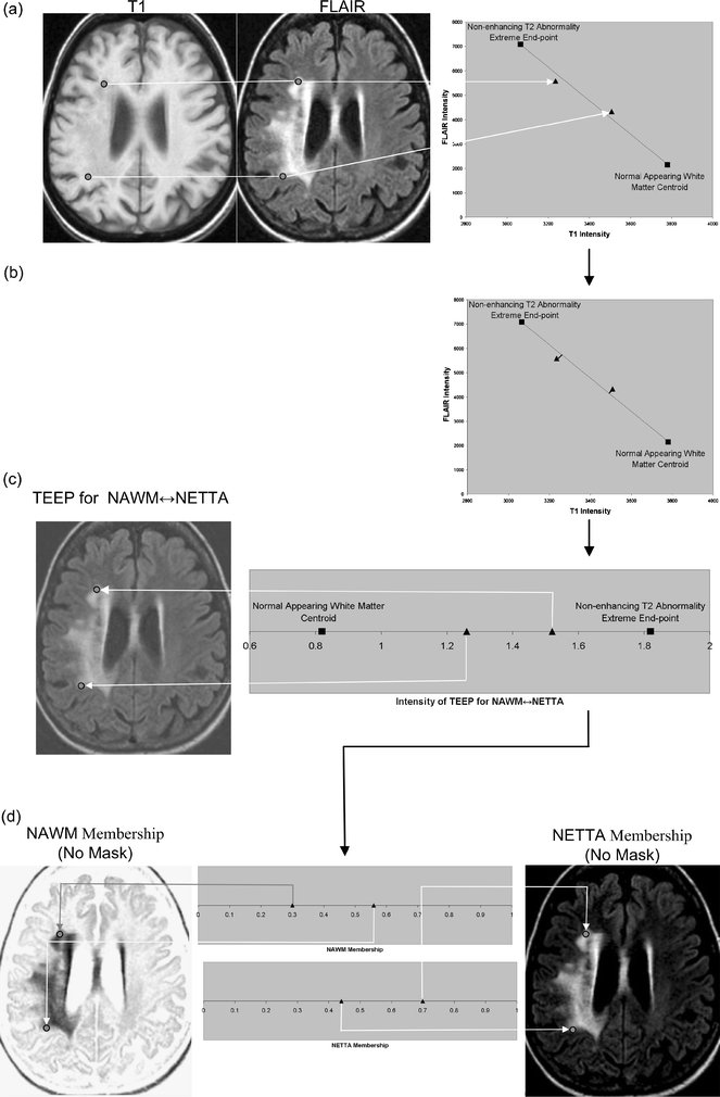
A feature extraction step is performed, which recombines the original volumes to create a volume for each tissue pair at each acquisition. Each of these recombined volumes will be referred to as a transition-emphasizing extraction product (TEEP). This process of feature extraction is accomplished by casting a line through the centroids of each relevant pair of tissues, and then perpendicularly projecting all points in feature space onto the resulting line. (a) The intensities of voxels may be shown in a scatterplot. For clarity, a two-dimensional feature space made up of T1 and FLAIR is shown, but all three volumes (T1, T1 Post-Gd, and FLAIR) were used in this study. The intensities of two selected points from the volume are plotted here to demonstrate a voxel containing moderate NETTA (lower point), and another voxel containing more pronounced NETTA (upper point). The line in feature space connecting the centroid of NETTA with the NAWM centroid is also shown, as are the centroids of these tissues. (b) The feature extraction is accomplished by projecting all voxels onto the line connecting the NAWM and NETTA centroids using equation 1. (c) The output volume, or TEEP, is thus produced for each tissue-pair and acquisition. Note that the values on the line have been shifted to the right by 0.82 in order to ensure that the lowest-valued voxel in the TEEP as a whole will be exactly 0.0. In the case shown, the TEEP appears similar to the FLAIR image because most of the contrast between NAWM and NETTA is held in the FLAIR image. Voxels that are not either NETTA or NAWM will be removed from consideration of NETTA–NAWM transition in a later step (not shown in this figure). (d) The TEEP represents both tissues in a tissue pair; this may be shown more clearly by converting the values in the TEEP volume to two membership volumes using equation 2. This process is shown graphically for the more anterior of the two points in Figure 4.

The second step in the change detection algorithm is a feature extraction step. Feature extraction is a process by which multidimensional data are mathematically combined to create a new data value. In the present study, the intensities of the original volumes (T1, T1 Post-Gd, and FLAIR) were combined mathematically to create one new volume for each dual-tissue class at each acquisition. In this study, the feature extraction step consisted of recombining the intensities of the original volumes on a voxel-by-voxel basis by perpendicularly projecting the intensities of each voxel in feature space onto lines connecting the centroids of the relevant tissue pairs (Fig. 3b). Equation 1 was used to effect this process. The process of feature extraction reduces dimensionality—these extracted volumes are what the algorithm uses, one at a time, to compute memberships, using equation 2, in a later step. The process of feature extraction also increases contrast and decreases noise. In addition to dimensionality reduction, noise reduction, and improved contrast, this process of feature extraction affords a degree of immunity against acquisition-related changes, as the end points of the transition lines are always formed by the centroids of the constituent tissues regardless of their absolute quantitative positions in multispectral image space.²⁴ The volumes which are created by this feature extraction process will be referred to as the transition-emphasizing extraction products (TEEPs) (Fig. 4).

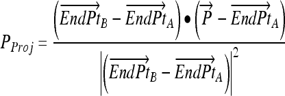1

= Line end point A

= Line end point B

= Point to be projected

P_Proj

= Projection of onto line

•

= Dot product

Fig 4.

Computing fractional membership from TEEPs. The line shown in the above figure corresponds to the NAWM↔NETTA TEEP from Figure 3c, and the point marked “x” corresponds to the more anterior of the two sample points. Within a given TEEP, the fractional membership is determined by the relative linear fractional distance from either end point. A voxel exactly on top of the NETTA end point would possess 1.0 membership in NETTA and 0.0 membership in NAWM, whereas the voxel situated at the marker shown would possess a membership of 0.7 in NETTA and 0.3 in NAWM. The symbols x, μ_A, and μ_B are provided for correspondence with equation 2.

Arrow indicates that quantity is a vector quantity. In this case, the vectors are made up of the multispectral intensities, i.e., T1, T1 Post-Gd, and FLAIR. The derivation of the above equation may be found elsewhere.²⁵

In the third step, the algorithm determines which dual-tissue class each voxel is most likely to belong to at each acquisition. This step is predicated on the assumption that voxels, which belong to a dual-tissue class, will lie close to that dual-tissue class’ partial membership line in the full original feature space. The step of assigning each voxel to a dual-tissue class amounts to a form of classification where the elongated “clusters” stretch from one pure tissue centroid to the other. The algorithm assumes Gaussian noise^26–34 and uses a transaxial Mahalanobis distance-based metric (equation 3) to determine the distance of a given voxel from the line in feature space corresponding to each dual-tissue class (Fig. 5). The algorithm then assigns each voxel to the dual-tissue class it is closest to, considering both baseline and follow-up acquisitions. It may also permit a temporary assignment to multiple partial membership lines if there exists sufficient ambiguity to warrant doing so; the resulting ambiguity in such a case is resolved in a subsequent step.

Fig 5.

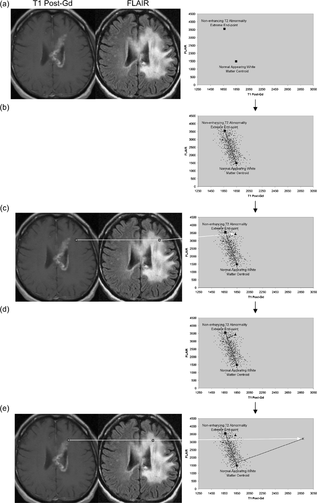
Computation of the transaxial Mahalanobis distance. As in Figure 3a, the end points of the line corresponding to the NAWM↔NETTA dual-tissue pair, which were derived from part 1 of the algorithm, may be plotted. (b) Based upon the samples of NAWM and “extreme” NETTA, the algorithm synthesizes sample points following the line connecting the two centroids but offsets by noise. These represent the locations in the scatterplot where the algorithm would expect to find real NETTA possessing varying degrees of T2 abnormality. (c) The location of one particular voxel of real NETTA, drawn from the images, is shown in the scatterplot for demonstration purposes. Its location on the scatterplot, as expected, falls within the range of the synthesized NETTA points. (d) The line originating from this point which is perpendicular to the NAWM↔NETTA partial membership line is determined. The inverse of the square of the Mahalanobis distance from the point to its perpendicular projection on the NAWM↔NETTA partial membership line is determined using equation 3. When points are members of a given dual-tissue class, this inverse of the Mahalanobis distance should be low (roughly speaking, within the range of the inverse of the Mahalanobis distance for NAWM↔NETTA points shown; however, description of the precise mechanism of thresholding is beyond the scope of this article). (e) The location of one particular real voxel containing enhancing tissue (i.e., definitively not a member of the NAWM↔NETTA dual-tissue class) is shown, and this point’s multispectral intensity is plotted on the scatterplot. As in step (d), the line which originates from this point and which is perpendicular to the NAWM↔NETTA partial membership line is determined. The inverse square of the Mahalanobis distance between the point and its perpendicular projection onto the NAWM↔NETTA partial membership line is again determined using equation 3. When points are not members of a given dual-tissue class, the inverse square of the transaxial Mahalanobis distance is high.

In the fourth step, the algorithm uses the TEEP volumes to compute the fractional membership of each voxel at each time point within each of the dual-tissue classes to which each voxel belongs. Recall that in step 2, feature extraction was accomplished by projecting voxels onto the partial membership lines. In step 3, it was determined which dual-tissue classes were consistent with the data. In the current step, the change over the possible dual-tissue classes is computed using the product of step 2. First, the extracted volumes from step 2 are converted to membership volumes. This is a simple transformation—the algorithm assumes that partial-volumed voxels possess a multispectral intensity equal to a weighted sum of the multispectral intensities of the constituent tissues, where the weight corresponding to each contributing tissue is equal to that tissue’s fractional volume.^{24,26,29–31,35–38} The reverse process, converting from fractional position between the two centroids corresponding to the tissue pair back to memberships (or fractional volumes), is accomplished using equation 2. Simple concrete examples of this are shown in Figures 3d and 4.

2

membership_Aand membership_B

: refer to the memberships, to be computed, in the two tissues making up a given partial membership line

x

: is the intensity of the voxel whose membership in the two tissues is to be computed,

μ_A

: is the mean intensity of the first tissue making up the partial membership line,

μ_B

: is the mean intensity of the second tissue making up the partial membership line (where x, μ_A, and μ_B are all intensities in the TEEP volume relevant to the given partial membership line).

The fifth step is a noise reduction step. Virtually every voxel will contain some variation in membership, from one time point to the next, strictly due to image noise. The algorithm makes use of the knowledge that real change occurs in a spatially coherent way, i.e., in the case of an actual change to the patient’s brain, voxels will tend to change in the same manner as their neighbors: one voxel previously containing NETTA, which develops enhancement, is not likely to be isolated—if the change is real, the voxel and its

3

D

: Mahalanobis distance

x

: A column vector containing the coordinate of the point whose Mahalanobis distance is to be computed

μ

: A column vector containing the coordinate of the perpendicular projection of the new point on the partial membership line of interest

V

: The covariance matrix of the synthesized partial membership points surrounding μ

 

More details regarding this equation may be found elsewhere. ³⁹

neighbors will acquire enhancement together. Change due to noise, however, will occur without such spatial coherence: a given voxel will be likely to be changing in a different way from its neighbors. Confidence in which of these is the source of an observed change is based on two measurements: spatial extent of a region of change and mean membership change within a region. The larger the spatial extent of an observed change, the greater the likelihood that it is real and not due to noise; and secondly, the greater the mean membership change of the region, the more likely the change is real and not due to noise. The algorithm identifies all regions of the image, which are changing in a spatially coherent manner, and then computes the mean change in membership over that region. The mean membership change is then compared to a threshold, which varies according to the spatial extent of the region (Fig. 6). If the mean membership change within a given region exceeds the threshold, the change is deemed real and is retained; otherwise, it is discarded. As shown in Figure 6, the threshold is based on a multiplier of the standard deviation of memberships in the given extracted feature/dual-tissue class, so the threshold varies according to the amount of noise actually present in the given dual-tissue class.

Fig 6.

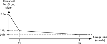
Relationship between the number of voxels in a given region the and standard deviation multiplier used by the spatially adaptive noise reduction routines. Smaller regions are required to possess a higher mean change than larger regions in order to be considered to be due to an underlying biological process and not due to noise. In the figure, “σ” is specific to the dual-tissue class in question and is determined by how much static voxels belonging to that partial membership line vary. Note that if the region of spatial coherence is sufficiently large, a mean change well below the noise floor will be correctly identified as real. The actual form of the threshold was determined empirically; more statistically rigorous approaches are possible.

Once the algorithm has identified regions it considers to contain real change, it generates output in two forms (bottom row in Fig. 2): a quantitative change map consisting of a series of volumes encoding membership changes (for quantitative analysis purposes), and a color-coded change map superimposed on the patient’s anatomical image (for visual inspection). In the color change map, regions which have been identified as changing are colored according to the type of change (Fig. 7). For example, orange corresponds to previously NAWM which has acquired enhancement from one scan to the next in the serial pair, whereas red corresponds to previously NAWM which has acquired NETTA. Note additionally that changes of the opposite type are assigned different colors for clarity, e.g., previously NAWM acquiring enhancement is colored orange, whereas previously enhancing tissue which is losing enhancing character is colored blue. It should be noted that the color scheme encodes change so that a voxel colored red need not be absolutely normal to begin with nor absolutely intense in T2 at follow-up. A given voxel might possess slightly abnormal T2 in the initial scan, have a slightly greater degree of abnormal T2 at the follow-up scan, and would therefore appear as a red of low intensity in the color coded change map. An example of a color-coded change map superimposed on a real patient image is shown in Figure 8.

Fig 7.

The color scheme used for all change detection images in this article. The color indicates the type of transition occurring, whereas the intensity indicates the size of change. Note that two colors correspond to each dual-tissue class because a change may proceed in either direction, e.g., previously, NAWM may develop increased enhancement (orange), and tissue which was already enhancing may also lose enhancing character (light blue, extreme upper left).

Fig 8.

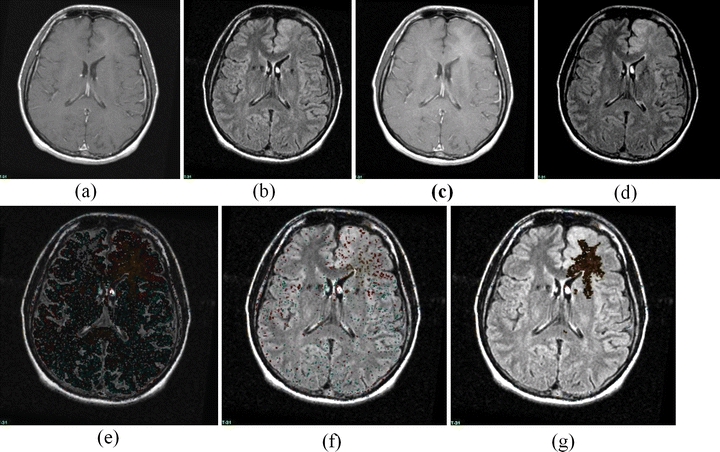
A sample change detection image, demonstrating the detection of changes which are subtle but which involve a large area. (a) T1 Post-Gd Time 0, (b) FLAIR Time 0, (c) T1 Post-Gd Time 1, (d) FLAIR Time 1, (e) Unthresholded color change map (which is dark because the change, while omnipresent, is of quite small membership). (f) Simple thresholded color change map, (g) adaptive thresholded change map. Note that the simple threshold has completely missed the change, but has not removed all noise, whereas the adaptive threshold technique eliminates virtually all noise and retains a large region of subtle change. The color scheme is shown in Figure 7; the region shown consists of an area of development of subtle enhancement.

Change Detection Phantom

In order to provide quantitative evaluation of the algorithm, a digital phantom was developed. The purpose of the phantom is to embody intensity characteristics as close as possible to those of actual images while possessing a known ground truth—i.e., the static memberships and actual changes are known. The phantom generation program models the intensities of mixtures of tissues as linear combinations of the intensities of the constituent tissues, as does the change detector algorithm.

The program to generate the phantoms used in this study begins with a set of membership volumes—each one corresponding to one of the tissues to appear in the phantom. For this study, these were: NAWM, gray matter, CSF, enhancement, necrosis, and NETTA. Voxels in the phantom contain mixtures of at most two tissues, and the mixtures occur in varying degrees. Mixtures of pathological tissues are represented, such as NAWM and NETTA, in addition to mixtures (i.e., simulated partial-volumed voxels) of normal tissues, such as gray matter and CSF. Mixtures of pairs of normal tissues are represented in increments of 20%, i.e., 100% gray matter/0% CSF, 80% gray matter/20% CSF, 60% gray matter/40% CSF, etc. Mixtures involving pathological tissues are represented in finer increments of 10%, i.e., 100% NAWM/0% NETTA, 90% NAWM/10% NETTA, 80% NAWM/20% NETTA, etc. Furthermore, while the mixtures of normal tissues remain static from one scan to the next in the serial pair, the mixtures of pathological tissues vary in discrete increments. Figure 9 shows source membership volumes and constructed phantom volumes for the synthetic baseline scans, and Figure 10 shows these volumes for the follow-up scans. Each grid contains 121 subelements to represent a variety of baseline and follow-up membership combinations for each tissue pair (11 mixtures of each pair at baseline×11 mixtures of each pair at follow-up). This wide variety of starting and stopping combinations facilitates testing of the change detector algorithm’s ability to identify changes not only of a variety of membership sizes and tissue pairs but additionally for a variety of baseline and follow-up states. This is important because (as an example) in real images, slightly edematous white matter may acquire a greater edematous character just as very edematous white matter may acquire a greater edematous character. Both of these changes have clinical importance.

Fig 9.

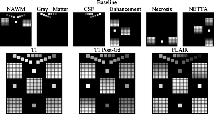
Construction of the baseline change phantom. The membership volumes for the desired phantom (top row) are used in conjunction with intensity samples derived from patient brain images (not shown) to generate the synthetic pulse sequences (bottom row). The largest squares show regions of pure tissues, all of which can be seen to be invariant in terms of membership from the baseline to the follow-up scan. The medium-sized squares contain mixtures of normal tissues, all of which also can be seen to possess invariant membership mixtures from one time point to the next. Each of the five grids contains mixtures of pathological tissues, with each grid corresponding to one of the dual-tissue classes.

Fig 10.

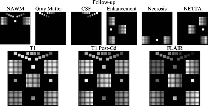
Construction of the follow-up change phantom. As in Figure 9, the membership volumes for the desired phantom (top row) are used to generate the synthetic pulse sequences (bottom row). Note the difference in orientation of the gradation within the grids at each time point. The result is a broad range of starting and stopping membership values over each grid/dual-tissue class.

For each voxel in the generated phantom volumes, equation 4 was used to convert membership volumes (top rows in Figs. 9 and 10) into synthetic images (bottom rows in Figs. 9 and 10). For the purposes of this study, intensity distributions from 18 patient exams were used to generate nine serial phantoms (each of the nine serial phantoms possessed both a baseline and a follow-up exam).

4

PS

: the pulse sequence to be simulated (T1, T1 Post-Gd, or FLAIR)

Random(x)

: refers to the intensity of a randomly selected voxel drawn from a real sample set for the given tissue and pulse sequence

Memb_Tissue

: the desired membership of the synthetic voxel in the given tissue

Benchmark for Detection of Change—A Simple Classify–Subtract Algorithm

To serve as a benchmark for the change detector algorithm described in this article, a simple classify–subtract algorithm was constructed. For each serial pair, this algorithm performs a simple supervised Mahalanobis-based classification of the multispectral volume set at each time point in a given serial pair to obtain a pair of membership volume sets. The algorithm then subtracts these. The classify–subtract algorithm also makes a two-tissue assumption, analogous to the two-tissue assumption made by the change detection algorithm. It first computes the change in membership over each tissue pair using the same set of dual-tissue classes used by the change detector algorithm. Obviously, as a result of noise, the precise changes in membership over these pairs are rarely exactly equal. In the almost universal case of inequality at a given voxel, the smaller of the two changes is used as the change in membership over the dual-tissue class. In keeping with the assumption of at most two tissues per voxel, only the dual-tissue class with the largest membership change is retained. Finally, for the purposes of noise reduction, the classify–subtract algorithm applies a flat threshold of 0.1 (10% change in membership) so that only membership changes of at least 10% are retained.

Phantom-Based Comparison of the Two Algorithms

For each of the nine serial phantom pairs, both the classify–subtract and the change detector algorithms were run. The specificity of both algorithms was computed, and additionally, two sensitivity measures were computed: one using a demanding criterion, and another using a lenient criterion. For the demanding criterion, a voxel was counted as “correct” if the algorithm not only identified correctly that it was changing but additionally identified the correct tissue pair which was involved. For the lenient criterion, a voxel was counted as “correct” if it was correctly detected to be changing without regard to whether the given algorithm correctly identified the correct tissue pair. P-values were computed for each of these metrics, comparing the performance of the classify–subtract algorithm with the performance of the change detector over all nine phantoms and testing the null hypothesis that there was no actual difference in performance. A two-tailed Wilcoxon signed-rank test was used to compute the P-value in all cases, with 0.05 used as the requisite level of significance.

RESULTS

Change Detection Phantom

The outputs for the classify–subtract algorithm, and the proposed change detection algorithm, are shown graphically in Figure 11 for each of the nine phantoms along with the actual change (upper left-hand corner of Fig. 11), all using the color scheme from Figure 7. Visually, it is apparent that the output of the proposed change detection algorithm more closely resembles the actual change compared with the output of the classify–subtract algorithm. Sensitivity (using both the demanding and the lenient criteria) and specificity are shown in Table 1. The absolute value of the mean errors was almost universally smaller for the change detector algorithm (min 0.0, max 0.031, median 0.0068) compared with the classify–subtract algorithm (min 0.000035, max 0.14, median 0.0235). Graphical depiction of the errors for phantom 1, over each dual-tissue class, is shown in Figure 12 and demonstrates that the errors associated with the novel change detection algorithm are much more regular and of smaller magnitude than those of the classify–subtract algorithm.

Fig 11.

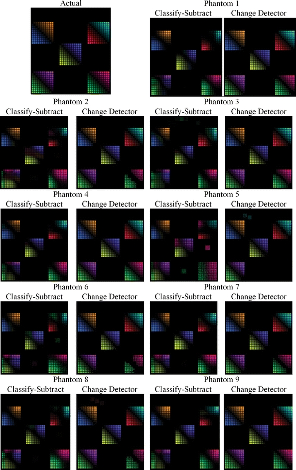
Ground truth output for the change detection phantom (upper left), and output for both the classify–subtract and the change detection algorithms for all nine serial phantoms.

Table 1.

Algorithm: CS Indicates Classify–Subtract; CD Indicates Change Detector

Phantom #	Algorithm	Sensitivity—Demanding Criteria (P=0.004)	Sensitivity—Lenient Criteria (P=0.008)	Specificity (P=0.035)
1	CS	0.62	0.71	0.96
	CD	0.93	0.93	1.00
2	CS	0.54	0.77	0.90
	CD	0.87	0.87	1.00
3	CS	0.62	0.77	0.90
	CD	0.94	0.94	1.00
4	CS	0.59	0.71	0.98
	CD	0.95	0.96	1.00
5	CS	0.55	0.77	0.80
	CD	0.68	0.71	0.94
6	CS	0.57	0.75	0.87
	CD	0.82	0.83	1.00
7	CS	0.65	0.78	0.95
	CD	0.90	0.90	1.00
8	CS	0.58	0.72	0.97
	CD	0.85	0.86	0.91
9	CS	0.62	0.74	0.98
	CD	0.94	0.94	1.00

P-values were computed using two-tailed Wilcoxon signed-rank test.

Fig. 12.

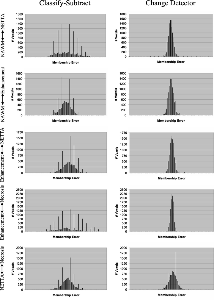
Histograms of errors for phantom 1 over each dual-tissue class. The x-axis labels (membership error) range from −1 to +1 for all charts, with the bin corresponding to zero error located at the center of each chart. The ideal histogram would be one in which there was a single bar in the center of each histogram, signifying that all voxels possessed zero error. The distributions of errors for the change detector appear more regular, Gaussian, and are centered on error=0.0 in all cases. The distributions of errors for the classify–subtract algorithm appear broader with bins located further from the center, signifying a greater number of voxels with larger error. The graphs corresponding to the classify–subtract algorithm additionally possess many large spikes, corresponding to voxels where the classify–subtract algorithm failed to correctly identify the dual-tissue class of voxels (the discreteness of these spikes results from the discreteness of the phantom’s underlying bins).

DISCUSSION

The detection and characterization of change in serial imaging studies of the brain is an important task. A number of approaches exist, including the current clinical standard of manual inspection and a variety of computational approaches which have been described in the literature. Manual inspection is easy to apply—anyone can look at a pair of images—but it is also notoriously noisy. Faced with the same images, even experts often disagree about the existence or nonexistence and nature of changes. A method that could overcome these problems could help objectively measure response to therapies, in order to guide their use in individual patients and additionally compare their action across populations. The algorithm proposed in this study embodies the beneficial aspects of many of the prior algorithms, and it has advantages which previous algorithms do not possess.³ The algorithm attempts to separate acquisition-related changes from pathology-related changes through feature extraction and spatially adaptive noise reduction. The algorithm is able to highlight very subtle changes (like subtraction) and produce localized descriptions of those changes (like subtraction and warping). It has the potential to reduce the amount of data which must be reviewed by the clinician, and the output of the algorithm is highly intuitive (unlike subtraction but like classify–subtract). It is relatively insensitive to normalization problems (unlike subtraction and warping but like classify–subtract). The proposed algorithm successfully suppresses noise (unlike subtraction).

Figure 12 clearly demonstrates the superiority of the change detector over classify–subtract: the output of the change detector more closely resembles the actual change image (shown in the upper left frame) than does the output of the classify–subtract algorithm. In the change detector case, each grid predominantly contains only two colors, and they are the correct colors for the dual-tissue class represented by that grid. In contrast, the classify–subtract algorithm often produces many colors for a single grid, which means that this algorithm would misinterpret an actual change of some given type as many different dual-tissue classes. The grid representing the enhancement↔necrosis pair (lower left corner of each phantom image) provides a striking example of this. In all nine phantoms, the classify–subtract algorithm has misclassified large numbers of voxels from this dual-tissue class into incorrect dual-tissue classes. The smooth gradation is also apparent for the proposed change detection algorithm from the diagonal possessing zero actual change to the upper right and lower left corners, which possess complete change from one tissue to another. This should be contrasted with the classify–subtract output, which shows “cold spots” on the one hand (no computed change when actual change is present) and “hot spots” on the other hand (computed change is larger than the actual change). This results from the classify–subtract algorithm’s use of a Mahalanobis distance-based classifier as the means for membership computation; using this metric, the computed membership of a given voxel is very nonlinear as it moves through feature space from one centroid to another. This demonstrates the value of separating tissue mixture assignment with a Mahalanobis distance-based classifier (step 3) and the separate computation of change in tissue fraction (step 4).

Turning to Table 1, which shows the sensitivity and specificity measures for the classify–subtract and change detector algorithms, the superior performance of the change detector compared with that of the classify–subtract algorithm is once again apparent. The superior sensitivity of the change detector algorithm is significant at a 0.05 level whether the change detector is required to correctly identify the type of change which is occurring (demanding criteria) or not (lenient criteria). Superior specificity was also observed for the proposed change detection algorithm. In seven out of nine cases, the change detector was able to achieve a perfect 1.0 specificity. The figures shown in Table 1 are truncated, not rounded, so 1.0 specificity represents a true perfect identification of all unchanging voxels. This is an important accomplishment because in serial brain MR, the vast majority of voxels will be unchanging whether or not there is actual change present somewhere in the image. The ability of a change detection algorithm to reject false positives facilitates both manual and automated inspection of change detection images.

Figure 12 shows the histograms of the errors over each dual-tissue class for the classify–subtract and change detection algorithms for phantom 1. The error distributions for the change detector are taller and narrower than those of the classify–subtract algorithm because most errors for the change detector algorithm are close to zero. The error distributions for the proposed change detection algorithm are also visibly more regular than those of the classify–subtract algorithm. The discrete spikes correspond to voxels for which the correct type of change was not determined. The discreteness of these spikes results from the discreteness of the actual changes in the phantom (which occur only in discrete membership increments of 10%). These spikes are much lower for the change detection algorithm than for the classify–subtract algorithm. For only one of the dual-tissue classes (NETTA↔necrosis) are there spikes for the change detector algorithm, which are comparable in height to those of the classify–subtract algorithm (the NETTA↔necrosis tissue pair was challenging for both algorithms because contrast between these two tissues is extremely low in comparison with noise, which makes identification of change difficult regardless of the algorithm).

The output of the proposed change detector algorithm is shown in Figures 13, 14, 15, 16 for four clinical cases. Corresponding output for the classify–subtract algorithm is not shown because like the proposed change detector algorithm, the classify–subtract algorithm requires samples of all tissues (normal and pathological); however, the classify–subtract algorithm does not possess a method to generate synthetic samples when none are available in the image, as does the change detection algorithm. Additionally, it should be noted that even when examples of all normal and pathological tissues are present, the classify–subtract algorithm performs poorly in the face of subtle changes, as demonstrated in the data in Figure 11. This figure also graphically demonstrates the high sensitivity of the change detection algorithm to change, with little susceptibility to noise in unchanging regions. The change detection algorithm can also produce quantitative measures of change, but validating these measures is beyond the scope of this paper. We present clinical cases in Figures 13, 14, 15, 16, as an indication that the high accuracy demonstrated in phantom work can be reasonably expected to be found in clinical cases.

Fig 13.

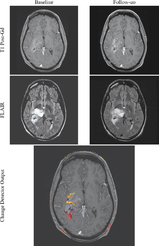
Subtle but important changes may hide in and around a lesion. The algorithm possesses the ability to identify and highlight such subtle changes.

Fig 14.

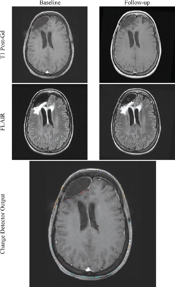
Confirmation of stability can be as difficult as the detection of change. The change detector’s ability to reject noise can help confirm the patient’s unchanging status.

Fig 15.

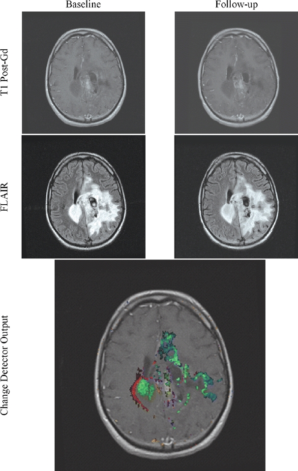
Change may be difficult to interpret because of the complexity of the lesion. Use of the change detector lessens this difficulty.

Fig 16.

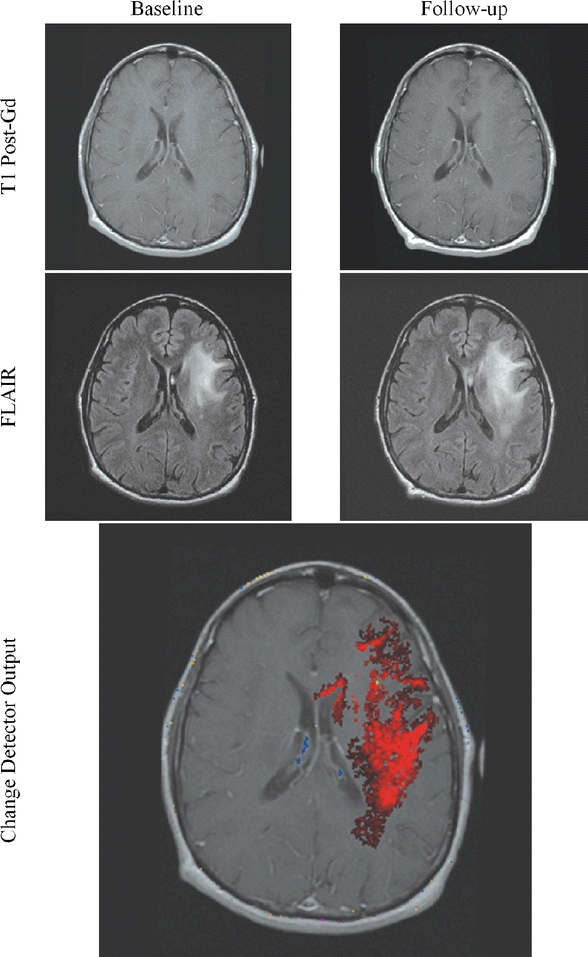
Change may be subtle in parts but more dramatic when taken as a whole.

Change detection and characterization in medical imaging is a relatively new field of imaging. It shows great promise to augment the capabilities of human observers by focusing their attention on limited regions within the potentially vast datasets being created today and by providing an objective measure of change that is immune to human variability.

CONCLUSIONS

We have described a highly automated algorithm which numerically compares two serial multispectral MR brain studies for the purposes of detecting and characterizing changes. Using a digital phantom, the algorithm has been compared to a simpler classify–subtract method. It has been demonstrated that the current algorithm is able to: (1) more accurately determine if voxels in serial examinations are changing, (2) define the category of change which is occurring, and (3) more accurately compute the membership change involved.

References

- 1.Simons DJ, Levin DT. Change blindness. Trends Cogn Sci. 1997;1:261–267. doi: 10.1016/S1364-6613(97)01080-2. [DOI] [PubMed] [Google Scholar]
- 2.Rensink RA. Change detection. Annu Rev Psychol. 2002;53:245–277. doi: 10.1146/annurev.psych.53.100901.135125. [DOI] [PubMed] [Google Scholar]
- 3.Patriarche J, Erickson B. A review of the automated detection of change in serial imaging studies of the brain. J Digit Imaging. 2004;17:158–174. doi: 10.1007/s10278-004-1010-x. [DOI] [PMC free article] [PubMed] [Google Scholar]
- 4.Radke RJ, Andra S, Al-Kofahi O, Roysam B. Image change detection algorithms: a systematic survey. IEEE Trans Image Process. 2005;14:294–307. doi: 10.1109/TIP.2004.838698. [DOI] [PubMed] [Google Scholar]
- 5.Miller AB, Hoogstraten B, Staquet M, Winkler A. Reporting results of cancer treatment. Cancer. 1981;47:207–214. doi: 10.1002/1097-0142(19810101)47:1<207::AID-CNCR2820470134>3.0.CO;2-6. [DOI] [PubMed] [Google Scholar]
- 6.Green S, Weiss G. Southwest oncology group standard response criteria, endpoint definitions and toxicity criteria. Invest New Drugs. 1992;10:239–253. doi: 10.1007/BF00944177. [DOI] [PubMed] [Google Scholar]
- 7.Ollivier L, Padhani AR. The RECIST (Response Evaluation Criteria in Solid Tumors) criteria: implications for diagnostic radiologists. Br J Radiol. 2001;74:983–986. doi: 10.1259/bjr.74.887.740983. [DOI] [PubMed] [Google Scholar]
- 8.Gehan EA, Tefft MC. Will there be resistance to the RECIST (Response Evaluation Criteria in Solid Tumors)? J Natl Cancer Inst. 2000;92:179–181. doi: 10.1093/jnci/92.3.179. [DOI] [PubMed] [Google Scholar]
- 9.Therasse P, Arbuck SG, Eisenhauer EA, Wanders J, Kaplan RS, Rubinstein L, Verweij J, Glabbeke M, Oosterom AT, Christian MC, Gwyther SG. New guidelines to evaluate the response to treatment in solid tumors. J Natl Cancer Inst. 2000;92:205–216. doi: 10.1093/jnci/92.3.205. [DOI] [PubMed] [Google Scholar]
- 10.Tsuchida Y, Therasse P. Response evaluation criteria in solid tumors (RECIST): new guidelines. Med Pediatr Oncol. 2001;37:1–3. doi: 10.1002/mpo.1154. [DOI] [PubMed] [Google Scholar]
- 11.Padhani AR, Husband JE. Are current tumour response criteria relevant for the 21st century? Br J Radiol. 2000;73:1031–1033. doi: 10.1259/bjr.73.874.11271893. [DOI] [PubMed] [Google Scholar]
- 12.Rusinek H, Leon MJ, George AE, Stylopoulos LA, Chandra R, Smith G, Rand T, Mourino M, Kowalski H. Alzheimer disease: measuring loss of cerebral gray matter with MR imaging. Radiology. 1991;178:109–114. doi: 10.1148/radiology.178.1.1984287. [DOI] [PubMed] [Google Scholar]
- 13.Weiner HL, Guttmann CR, Khoury SJ, Orav EJ, Hohol MJ, Kikinis R, Jolesz FA. Serial magnetic resonance imaging in multiple sclerosis: correlation with attacks, disability, and disease stage. J Neuroimmunol. 2000;104:164–173. doi: 10.1016/S0165-5728(99)00273-8. [DOI] [PubMed] [Google Scholar]
- 14.Jack CR, Petersen RC, Xu Y, O’Brien PC, Smith GE, Ivnik RJ, Tangalos EG, Kokmen E. Rate of medial temporal lobe atrophy in typical aging and Alzheimer’s disease. Neurology. 1998;51:993–999. doi: 10.1212/wnl.51.4.993. [DOI] [PMC free article] [PubMed] [Google Scholar]
- 15.Rey D, Subsol G, Delingette H, Ayache N. Automatic detection and segmentation of evolving processes in 3D medical images: Application to multiple sclerosis. Med Image Anal. 2002;6:163–179. doi: 10.1016/S1361-8415(02)00056-7. [DOI] [PubMed] [Google Scholar]
- 16.Thompson PM, Giedd JN, Woods RP, MacDonald D, Evans AC, Toga AW. Growth patterns in the developing brain detected by using continuum mechanical tensor maps. Nature. 2000;404:190–193. doi: 10.1038/35004593. [DOI] [PubMed] [Google Scholar]
- 17.Freeborough PA, Fox NC. Modeling brain deformations in Alzheimer disease by fluid registration of serial 3D MR images. J Comput Assist Tomogr. 1998;22:838–843. doi: 10.1097/00004728-199809000-00031. [DOI] [PubMed] [Google Scholar]
- 18.Thirion JP, Calmon G. Deformation analysis to detect and quantify active lesions in three-dimensional medical image sequences. IEEE Trans Med Imag. 1999;18:429–441. doi: 10.1109/42.774170. [DOI] [PubMed] [Google Scholar]
- 19.Gerig G, Welti D, Guttmann CRG, Colchester ACF, Székely G (1998) Exploring the Discrimination Power of the Time Domain for Segmentation and Characterization of Lesions in Serial MR Data. MICCAI, Boston, MA, pp 469–480 [DOI] [PubMed]
- 20.Meier DS, Guttmann CR. Time-series analysis of MRI intensity patterns in multiple sclerosis. Neuroimage. 2003;20:1193–1209. doi: 10.1016/S1053-8119(03)00354-9. [DOI] [PubMed] [Google Scholar]
- 21.Sled JG, Zijdenbos AP, Evans AC. A nonparametric method for automatic correction of intensity nonuniformity in MRI data. IEEE Trans Med Imag. 1998;17:87–97. doi: 10.1109/42.668698. [DOI] [PubMed] [Google Scholar]
- 22.National Library of Medicine Bethesda, MD. http://www.itk.org [DOI] [PubMed]
- 23.Mayo Clinic (2005) Rochester, MN. http://www.mayo.edu/bir/software/Analyze/Analyze1NEW.html
- 24.Soltanian-Zadeh H, Windham J, Peck D. Optimal linear transformation for MRI feature extraction. IEEE Trans Med Imag. 1996;15:749–767. doi: 10.1109/42.544494. [DOI] [PubMed] [Google Scholar]
- 25.Freidberg SH, Insel AJ. Introduction to Linear Algebra with Applications. Englewood Cliffs, NJ: Prentice-Hall; 1986. [Google Scholar]
- 26.Soltanian-Zadeh H, Windham J, Peck D, Yagle A. A comparative analysis of several transformations for enhancement and segmentation of magnetic resonance image scene sequences. IEEE Trans Med Imag. 1992;11:302–318. doi: 10.1109/42.158934. [DOI] [PubMed] [Google Scholar]
- 27.Castro JB, Tasciyan TA, Lee JN, Farzaneh F, Riederer SJ, Herfkens RJ. MR subtraction angiography with a matched filter. J Comput Assist Tomogr. 1988;12:355–362. doi: 10.1097/00004728-198803000-00037. [DOI] [PubMed] [Google Scholar]
- 28.Brown DG, Lee JN, Blinder RA, Wang HZ, Riederer SJ, Nolte LW. CNR enhancement in the presence of multiple interfering processes using linear filters. Magn Reson Med. 1990;14:79–96. doi: 10.1002/mrm.1910140109. [DOI] [PubMed] [Google Scholar]
- 29.Siadat M, Soltanian-Zadeh H. Partial volume estimation: an improvement for eigenimage method. SPIE Med Imag. 2000;3979:646–655. doi: 10.1117/12.387726. [DOI] [Google Scholar]
- 30.Laidlaw DH, Fleisher KW, Barr AH. Partial-volume Bayesian classification of material mixtures in MR volume data using voxel histograms. IEEE Trans Med Imag. 1998;17:74–86. doi: 10.1109/42.668696. [DOI] [PubMed] [Google Scholar]
- 31.Soltanian-Zadeh H, Windham J, Yagle A. Optimal transformation for correcting partial volume averaging effects in magnetic resonance imaging. IEEE Trans Nucl Sci. 1993;40:1204–1212. doi: 10.1109/23.256737. [DOI] [Google Scholar]
- 32.Lee JN, Riederer SJ. The contrast-to-noise in relaxation time, synthetic, and weighted-sum MR images. Magn Reson Med. 1987;5:13–22. doi: 10.1002/mrm.1910050103. [DOI] [PubMed] [Google Scholar]
- 33.McVeigh ER, Henkelman RM, Bronskill MJ. Noise and filtration in magnetic resonance imaging. Med Phys. 1985;12:586–591. doi: 10.1118/1.595679. [DOI] [PMC free article] [PubMed] [Google Scholar]
- 34.Buxton RB, Greensite F. Target-point combination of MR images. Magn Reson Med. 1991;18:102–115. doi: 10.1002/mrm.1910180112. [DOI] [PubMed] [Google Scholar]
- 35.Soltanian-Zadeh H, Peck D. Feature space analysis: Effects of MRI protocols. Med Phys. 2001;28:2344–2351. doi: 10.1118/1.1414306. [DOI] [PubMed] [Google Scholar]
- 36.Soltanian-Zadeh H, Windham J, Peck D, Mikkelsen T. Feature space analysis of MRI. Magn Reson Med. 1998;40:443–453. doi: 10.1002/mrm.1910400315. [DOI] [PubMed] [Google Scholar]
- 37.Windham J, Abd-Allah MA, Reimann DA, Froelich JW, Haggar AM. Eigenimage filtering in MR imaging. J Comput Assist Tomogr. 1988;12:1–9. doi: 10.1097/00004728-198801000-00001. [DOI] [PubMed] [Google Scholar]
- 38.Haggar AM, Windham JP, Reimann DA, Hearshen DO, Froelich JW. Eigenimage filtering in MR imaging: An application in the abnormal chest wall. Magn Reson Med. 1989;11:85–97. doi: 10.1002/mrm.1910110108. [DOI] [PubMed] [Google Scholar]
- 39.Manly B. Multivariate statistical methods a primer second. New York: Chapman & Hall; 1986. [Google Scholar]