Collective cell motion in endothelial monolayers

Abstract

Collective cell motility is an important aspect of several developmental and pathophysiological processes. Despite its importance, the mechanisms that allow cells to be both motile and adhere to one another are poorly understood. In this study we establish statistical properties of the random streaming behavior of endothelial monolayer cultures. To understand the reported empirical findings, we expand the widely used cellular Potts model to include active cell motility. For spontaneous directed motility we assume a positive feedback between cell displacements and cell polarity. The resulting model is studied with computer simulations, and is shown to exhibit behavior compatible with experimental findings. In particular, in monolayer cultures both the speed and persistence of cell motion decreases, transient cell chains move together as groups, and velocity correlations extend over several cell diameters. As active cell motility is ubiquitous both in vitro and in vivo, our model is expected to be a generally applicable representation of cellular behavior.

1. Introduction

Cell motility is instrumental both in development and certain pathophysiologies [1, 2]. Collective motility of interacting cells is a poorly understood, but fundamental aspect of these phenomena [3]. Such movements are required for important morphogenetic and pathological processes, for example, gastrulation, vasculogenesis, tumor growth, wound healing and revascularization of damaged tissues.

Arguably, cell sorting is the best studied process involving simultaneous displacement of closely packed cells [4, 5]. The differential adhesion hypothesis and its computational representations – based on the Potts model [6] or analogous lattice-free variants [7, 8] – successfully explain the outcome as well as the time-course of cell sorting experiments. The cell types used in sorting experiments move diffusively within bulk uniform environments far from cell type boundaries [4], although some temporal and spatial correlations are detectable [5].

Less is known how polarized cells, which maintain their migratory direction in time, move in high density cultures. Most studies addressing this problem have investigated the expansion of epithelial cell sheets or other monolayers into an empty area or `wound'. During the expansion, cells at the monolayer boundary [9] or within a broader layer [10] exert substantial traction forces and are thought to pull the passive bulk of the sheet forward [4, 11].

Recent studies on the motion of kidney epithelial (MDCK, [12]) or endothelial (HUVEC, [13]) cells within monolayers, as well as immune cells in explanted lymph nodes [14] have indicated an intriguing motion pattern. These cells exhibit an apparently undirected, albeit correlated, streaming behavior even in the absence of directed expansion of the whole monolayer. This type of motion is clearly different from both the uncorrelated diffusive activity of cell sorting experiments as well as from the external chemotactic gradient-driven motility.

In this study we establish statistical properties of the collective streaming motion within endothelial cell monolayers and introduce a suitable generalization of the widely-applied Potts model to describe a dense population of actively moving cells.

2. Empirical Results

To analyze movement patterns within endothelial cell monolayers, we studied cultures of three different kinds of endothelial cells – bovine capillary (BCE), bovine aortic (BAEC) and human umbilical cord vein (HUVEC) – on Matrigel- or fibronectin-coated tissue culture plastic (see Table I for details). Confluent cultures, under conditions favorable for cell motility were recorded for 24 hours using an automatized optical microscopy apparatus. A representative set of the resulting image sequences were analyzed by an automatic cell tracking procedure. As trajectories in Fig. 1 and supplementary Movie 1 demonstrate, endothelial cells form streams in monolayers: 5–20 cells move together in narrow, chain-like groups. The monolayers contain vortices, and adjacent streams moving in opposite directions. The resulting shear lines separate cells with substantial velocity differences.

Table 1.

Experimental data

Cell type	Substrate	Fields recorded/ analysed	S [μm/h]	Tp [min]	cell density [1000/cm2]	V(x) sample size [cell]
BAEC	Matrigel	36 / 9	33 ±2	33 ±3	80	1100
BCE	Matrigel	10 / 4	13 ±3	40 ± 10	40	500
HUVEC	Matrigel	10 / 3	14 ±2	112 ± 48	40	600
HUVEC	Matrigel	10 / 2	14 ±2	110 ± 50	20	500
HUVEC	Fibronectin	10 / 2	14 ±2	220 ± 170	70	1000
HUVEC	T.C. plate	10 / 2	18.3 ± 0.3	49 ± 7	40	N.A.

Figure 1.

Cell movement within a BAEC monolayer is visualized through cell trajectories. (a): A velocity field snapshot is indicated by short trajectories, obtained during 30 minutes. Cell centers are designated by black dots. Blue arrows show groups of cells moving together in streams. (b): A phase-contrast image detail with superimposed cell trajectories depicting movements during one hour. The average cell speed is 35 μm/h. Red-to-green colors indicate progressively later trajectory segments. Adjacent BAEC streams moving in opposite directions are separated by white lines, vortices are denoted by asterisks.

To better understand this collective cell flow characteristic for endothelial monolayers, below we calculate widely used and new statistical measures of individual and group cell motion. These measures facilitate the comparison of various experimental systems exhibiting streaming behavior, and are also needed to test computational models aiming to explain the phenomenon.

2.1. Individual cell movement statistics

The motion of individual cells is often evaluated in terms of average cell displacement [15, 16], d, over a time period t as

$$d^2\left(t\right)={\langle {({\mathit{X}}_i(t+t_0)-{\mathit{X}}_i\left(t_0\right))}^2\rangle }_i,$$ (1)

where X_i(t) denotes the center of cell i at time t, 〈…〉_i is an average over all possible cells, and t₀ is an arbitrary reference frame of the image sequence analyzed. The empirical d(t) curves indicate a persistent random walk behavior in endothelial monolayer cultures: the average displacements are well fitted by

$$d^2\left(t\right)=4D\left[t-T_p(1-e^{-t∕T_p})\right],$$ (2)

where T_p is the persistence time and D is the diffusion coefficient of the long-term random behavior (Table I). Thus, for short time periods cells move at a constant speed, S, as the distance is proportional with the time elapsed, while the motion is diffusive when investigated over a long time frame:

$$d\left(t\right)\approx \{\begin{array}{cc}\hfill St=\sqrt{\frac{2D}{T_p}}t,\hfill & \hfill \text{for}t⪡T_p\hfill \\ \hfill 2\sqrt{Dt},\hfill & \hfill \text{for}t⪢T_p.\hfill \end{array}\phantom{\}}$$

The fitted parameter values, summarized in Table I, scatter considerably: by a factor of two (S) and five (T_p) depending on the cell line and substrate combination used.

2.2. Average flow fields

As cells of a monolayer constrain the possible movements in their vicinity, correlation is expected in the motion of adjacent cells. In particular, immediately in front of a moving cell movement in the opposite direction (i.e., towards the cell) is unsustainable and therefore expected to be rare. Unfortunately, there are no established statistical descriptions of streaming cell motility. The co-moving domains are local and randomly oriented within the whole cell culture. Therefore, the large-scale rotational symmetry of the system is retained and spatial autocorrelation functions (see, e.g., Eq. 3 in [12]) depend only on the magnitude and not on the direction of their argument. Thus, such functions are ill-suited to describe the witdh and length of streams.

We suggest here V (x), the average flow field around moving cells, as a measure sensitive to the local cell movement pattern. For a given configuration of cell positions and velocities this procedure assigns reference systems co-aligned with the movement of each cell, and averages the velocity vectors observed at similar locations x (e.g., immediately in front, behind, left and right). The vectors of V (x) diminish in a hypothetical ensemble of statistically independent cells, as they are averages of independent random vectors.

To calculate V (x), for each cell i at time t the whole configuration is rotated around X_i so that ΔX_i, the displacement of cell i, is aligned to a reference direction φ = 0 (Fig. 2). The rotated displacement vectors are then binned according to a two-dimensional lattice B. The procedure is repeated for every cell i and multiple time points, and the bins are averaged resulting in a population- and time-averaged displacement field V (x). The procedure is further detailed in the Methods section.

Figure 2.

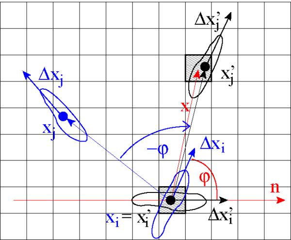
Calculation of the flow field V (x). The image depicts the process for two cells, i and j. The original configuration is drawn with blue color. Positions X_i and X_j denote cell centers, the vectors ΔX_i and ΔX_j are cell displacements. Cell i is heading in the direction φ, relative to an arbitrarily selected reference direction n. To calculate the flow field around cell i, first the configuration is rotated around X_i by –φ. In the rotated configuration (drawn in black) cell i is heading towards the reference direction (n). The center of cell j, ${\mathit{X}}_j^{\prime }$, now falls in the vicinity of lattice point x and therefore is taken into account for the average of V (x). The vicinity, B(x) is defined as a two dimensional bin (shaded area) centered at lattice site x. The procedure is then repeated for each cell and V (x) is calculated as an average over all cells i and j for which ${\mathit{X}}_j^{\prime }-{\mathit{X}}_i^{\prime }\in B\left(\mathit{x}\right)$ holds. Finally, the bins are also averaged over different time frames.

The averages were calculated from at least 30 independent data values per grid point, and we represent the estimated SEM values by a color code. The robustness of this statistical measure is demonstrated by comparing the flow fields of two consecutive time segments of culture recordings exhibiting similar behavior (Supplementary Fig. 1).

In Fig. 3 we plotted representative flow fields obtained from cultures with various cell-ECM combinations and cell densities (see Table I for culture parameters). Thus, Fig. 3 includes data from both high density monolayer cultures (panels a–d) and a subconfluent, lower density culture as a comparison (panel e). For a better comparison of the flow fields, in Fig. 4 we present the parallel component of V (x) along two orthogonal lines, one parallel (x axis) and one perpendicular (y axis) to the direction of motion.

Figure 3.

Monolayers of various endothelial cells exhibit similar flow fields on both Matrigel and fibronectin substrates. The local spatial correlation of cell movements were characterized by V (x), the average flow field that surrounds moving cells. Arrows indicate velocities as one-hour-displacements, the green arrow in the origin represents the average velocity of cells. For better visibility, vector lengths are scaled by a factor of five. Cultures with sufficient density (a–d) show streaming behavior, indicated by the similarity of average velocity vectors obtained in front of and behind the moving cells. The co-movement drops rapidly in the lateral direction, an indication of the local asymmetry of the streams. In a subconfluent culture (e) the correlation structure is less pronounced. The color code indicates the estimated relative SEM of the vectors: black corresponds to zero, yellow indicates 1, i.e., a SEM equal to the norm of the vector. A corresponding phase-contrast image of the cultures are shown in the right.

Figure 4.

Empirical flow field profiles along two orthogonal axes. To compare data presented in Fig. 3, we plotted the parallel (V_x) component of the average velocity vectors along the axes parallel (x, panel a) and perpendicular (y, panel b) to the direction of motion. To reduce symbol overlap, individual data sets are slightly shifted horizontally.

Flow fields derived from monolayer cultures reveal the presence of velocity correlations exceeding a spatial range of 200 μm, much larger than the typical cell diameter (mean distance between adjacent cell centers) of 30–40 μm. Streaming behavior is indicated by the similarity of average velocity vectors obtained within an elongated area surrounding the origin. In the lateral direction, the average velocity drops quickly and in some cases reverses direction (Fig. 4) – an indication that streams are narrow and adjacent streams move in opposite directions. Remarkably, very similar correlation structures are seen in all three types of endothelial cell monolayer cultures investigated, irrespective of the underlying extracellular matrix substratum used. In subconfluent cultures, where fewer constraints are imposed by the behavior of adjacent cells, the correlated (co-moving) area shrinks (Fig. 3e).

2.3. Separation of adjacent cells

Another, longer-term property of collective flow is its ability to maintain adjacency of cells. The amount of mixing within the monolayer is indicated by how quickly initially adjacent cells separate from each other. Thus, we calculated d₂, the average distance between cell pairs that are adjacent in a reference frame t₀:

$$d_2^2\left(t\right)={\langle {({\mathit{X}}_i\left(t\right)-{\mathit{X}}_i\left(t\right))}^2\rangle }_{(i,j)\in Q},$$ (3)

where 〈…〉 denotes average over all cell pairs i and j that are neighbors at the reference frame t₀ (the set Q).

As the average distances of 100 independent cell pairs reveal (Fig. 5a), cells approach and separate in a symmetric process, and the duration of their adhesion (if any) is not resolved well in our analysis. The di erences seen in Fig. 5a originate primarily from differences in cell speeds: when neighbor separation is plotted against the path length (time scaled by average velocity S), the three data sets collapse around the origin (Fig. 5b).

Figure 5.

Cell separation within the monolayers. (a): Average separation, d₂(t), of cells adjacent at time zero. (b): Increase in separation from the average cell size value d₂(t₀) versus the path length (time scaled by mean velocity). (c): Separation, d₂(t), versus the average displacement of cells, d(t). The blue line of slope $\sqrt{2}$ indicates an uncorrelated movement of cell pairs as derived in (5). Error bars indicate SEM.

It is natural to compare changes in cell-cell distance d₂ to the mean cell displacements d (Fig. 5c). When the separation is large compared to the initial distance of the cell pair, (3) can be approximated as

$$\begin{array}{cc}\hfill d_2^2\left(t\right)& \approx \langle {\left[({\mathit{X}}_i\left(t\right)-{\mathit{X}}_i\left(t_0\right))-({\mathit{X}}_j\left(t\right)-{\mathit{X}}_j\left(t_0\right))\right]}^2\rangle \hfill \\ \hfill & =2d^2\left(t\right)-2\langle ({\mathit{X}}_i\left(t\right)-{\mathit{X}}_i\left(t_0\right))({\mathit{X}}_j\left(t\right)-{\mathit{X}}_j\left(t_0\right))\rangle \hfill \end{array}$$ (4)

where the averages are calculated over the cell pairs (i, j) ε Q. For independent cell movements the last term in (4) vanishes, thus

$$d_2\left(t\right)\approx \sqrt{2d}\left(t\right)$$ (5)

holds asymptotically. Therefore, in Fig. 5c the asymptotic linear relation between average cell displacement and neighbor separation with a slope of $\sqrt{2}$ indicates a substantial mixing and an uncorrelated long-term behavior within the monolayer.

Our statistical characterization thus revealed that endothelial monolayers move in locally anisotropic, 50–100 μm wide and 200–300 μm long streams, which form and disappear at random positions. In low density cell cultures cells in front of a moving cell tend to move in similar direction, but cell movements in lateral directions are uncorrelated. Despite the presence of streams, cell mixing is substantial in the monolayers: with a good approximation, movement of adjacent cells can be considered as independent persistent random walks.

3. Model definition

3.1. Cellular Potts model

To explain and model the emergence of collective flow patterns in cell monolayers, we adopted the two dimensional cellular Potts model (CPM) approach. In theoretical studies the CPM is a frequently used method to represent the movement of closely packed cells [6, 17, 18, 14, 19, 20]. The main advantage of the CPM approach is that cell shape is explicitly represented; thus, the simulation has the potential to describe dynamics in which controlled cell shape plays an important role [17, 21]. To obtain a biologically plausible, yet simple, model we consider below a positive feedback loop between cell polarity and cell movement in addition to the surface tension-like intercellular adhesion and cell compressibility. As we explain in detail below, the model assumptions are the following:

• A1Cells form a monolayer and each cell is simply connected.
• A2Each cell has an approximately constant, pre-set size.
• A3Cells adhere to their neighbors.
• A4Each cell is capable of autonomous biased random motion. The direction bias (in a homogeneous environment) is set by an internal polarity vector.
• A5The polarity vector has a finite lifetime, but it is reinforced by co-directional displacements of the cell.

In the CPM a non-negative integer value σ is assigned to each lattice site x of a two-dimensional grid. Two lattice sites are considered neighbors if they share a side (primary neighbors) or connect via a corner (secondary neighbors). Cells are represented as simply connected domains, i.e., a set of adjacent lattice sites sharing the same label σ. The label is equal to the cell index i (0 < i ≤ N, where N is the number of cells in the simulation). Sites that belong to the irregularly shaped area devoid of cells are marked by the special value σ = 0.

Cell movement is the result of a series of elementary steps. Each step is an attempt to copy the spin value onto a random lattice site b from a randomly chosen adjacent site a, where σ(a) ≠ σ(b). This elementary step is executed with a probability p(a → b). If the domains remain simply connected (A1), and thus cells do not break apart or form voids, the probability assignment rule ensures the maintenance of a target cell size (A2), adhesion of cells (A3) and active cell motion (A4, A5). For convenience and historical reasons p is given as

$$\text{In}p(\mathit{a}\to \mathit{b})=\text{min}[0,-\Delta u(\mathit{a}\to \mathit{b})+w(\mathit{a}\to \mathit{b})],$$ (6)

where, as specified below in detail, w represents a bias responsible for the cell-specific active behavior considered, u represents a goal function to be minimized, and Δ(a → b) represents its change during the elementary step considered.

Since updating each lattice position takes more steps in a larger system, the elementary step cannot be chosen as the measure of time. The usual choice for time unit is the Monte Carlo step (MCS), defined as L² elementary steps, where L is the linear system size [21].

3.2. Evaluating configurations

In the CPM approach, a goal function (`energy') is assigned [6] to each configuration. The goal function guides cell behavior by distinguishing between favorable (low u) and unfavorable (high u) configurations as

$$u=\sum _{<\mathit{x},{\mathit{x}}^{\prime }>}{J}_{\sigma \left(\mathit{x}\right),\sigma \left({\mathit{x}}^{\prime }\right)}+\lambda \sum _{i=1}^N\delta A_i^2.$$ (7)

The first term in (7) enumerates cell boundary lengths. The summation goes over adjacent lattice sites. For a homogeneous cell population the J_i,j interaction matrix (0 ≤ i, j ≤ N) is given as

$$J_{i,j}=\{\begin{array}{ccc}0,\hfill & \text{for}i=j\hfill & \hfill \\ \alpha ,\hfill & \text{for}ij>0\text{and}i\ne j\hfill & \left(\text{intercellular boundary}\right)\hfill \\ \beta ,\hfill & \text{for}ij=0\text{and}i\ne j\hfill & \left(\text{free cell boundary}\right).\hfill \end{array}\phantom{\}}$$ (8)

The surface energy-like parameters α and β characterize both intercellular adhesiveness and cell surface fluctuations in the model. The magnitude of these values determines the roughness of cell boundaries: small magnitudes allow dynamic, long and hence curvy boundaries, while large magnitudes restrict boundaries to straight lines and thus freeze the dynamics. In addition to cell boundary roughness, the parameters α and β also specify the preference of intercellular connections over free cell surfaces (A3). If two adhering cells are separated by inserting a layer of empty sites between them, then the change in u is proportional to 2β – α at each site along the boundary line affected. Therefore, for 2β > α free cell boundaries are penalized and the cells are adhesive [22].

The second term in expression (7) is responsible for maintaining a preferred cell area (A2). For each cell i, the deviation of its area from a pre-set value is denoted by δA_i. Parameter λ adjusts the tolerance for deviation. Thus, λ is related to the compressibility of cells in the 2D plane, and also determines the magnitude of cell area fluctuations.

3.3. Cell polarity and active motility

While u evaluates configurations, w is assigned directly to the elementary steps and therefore allows the specification of a broader spectrum of cellular behavior [23]. Active cell motility involves cell polarity, a morphological, dynamical and biochemical difference between the cell's leading edge and tail [24, 25]. In this study we model active cell motility by first assigning a cell polarity vector p_k to each cell k (A4). We then increase the probability of those elementary conversion steps that advance the cell center in the direction parallel to p_k (Fig. 1), as

$$w(\mathit{a}\to \mathit{b})=P\sum _{k=\sigma \left(a\right),\sigma \left(b\right)}\frac{\Delta {\mathit{X}}_k(\mathit{a}\to \mathit{b}){\mathit{p}}_k}{\mid {\mathit{p}}_k\mid }.$$ (9)

Parameter P sets the magnitude of the bias and ΔX_k represents the displacement of the center of cell k during the elementary step considered.

The cell polarity vector is an attempt to represent the localization and magnitude of the biochemical changes characterizing the leading edge of a migratory cell. It is not yet clear what is the molecular polarization mechanism in endothelial cells. The best documented front/rear polarization mechanisms involve either the mutual inhibition of Rac and Rho, key GTPase `switches' of cell motility [1, 26], and/or the accumulation of the phosphatidyl-inositol membrane component PIP₃ [27, 28]. The accumulation of active Rac1 (and PIP₃) at the leading edge is thought to activate a biochemical cascade that involves the Arp2/3 complex providing new actin nucleation sites. The Rac1-Arp2/3 cascade eventually results in a local increase in actin polymerization, pushing the plasma membrane forward [27, 1]. Through positive feedback loops, both the Rac/Rho and PIP₂/PIP₃ systems are thought to be able to amplify slight spatial differences in upstream inputs and even develop a spontaneous polarity [27, 28]. This amplification of presumably random receptor activity and the related spontaneous symmetry breaking could explain the onset of spontaneous cell motility in a homogeneous environment, and motivates the use of a unit vector in rule (9).

Even less molecular details are known about what drives changes in cell polarity in the absence of external cues such as chemoattractant gradients. However, in a motile cell the polarization direction must change eventually. For instance, when the advance of the leading process is impaired and the process collapses, a new migration direction is selected and cell polarity is altered. We propose to update the cell polarity vectors by considering a spontaneous decay and a reinforcement from cell displacements (A5). In each MCS the change in p_k is

$$\Delta {\mathit{p}}_k=-r{\mathit{p}}_k+\Delta {\mathit{X}}_k,$$ (10)

where r is the rate of spontaneous decay and ΔX_k is the displacement of the center of cell k during the MCS considered. A characteristic memory length T of the polarization vector is defined as T = 1/r.

Rules (9) and (10) together constitute a positive feedback loop. In this model, steric constraints may result in co-migration of adjacent cells as the retraction of one cell allows for the expansion of the other. The resulting expansion of cell bodies (like the actin polymerization process in real cells) therefore can alter and synchronize cell polarity. The molecular mechanism for cell polarity reinforcement by cell motility may involve either the stabilization of PIP₃ accumulation by actin polymerization [29, 30, 31], or the activation of Rac1 by microtubule dynamics [32, 33].

4. Simulation Results

We have chosen the open source Tissue Simulation Toolkit ([34, 21]) as our CPM framework, in which we implemented our extensions as C++ codes. We refrain from using a temperature-like parameter, as rule (3) of [6], analogous to our rule (6), simply scales each CPM parameter α, β and λ by the temperature, a constant. Thus, when comparing our studies with those that include a temperature in the simulations, our parameter values are to be compared with the corresponding values divided by the temperature.

Model simulations with N = 1000 cells were performed in a 200 × 200 lattice, with parameters α = 2, λ = 1 and P = 2, T=5 MCS (see Table II for a summary of the parameter values used). After scaling by temperature, our parameters are within the same range as those in previous studies [6, 21, 35, 20]. We applied closed boundary conditions (immutable empty sites at the border) in the simulations.

Table 2.

Parameters used in the model

Parameter name	Symbol	Value	Range	Main, experimentally detectable effect (s)
Cell-cell boundary cost	α	2	1–4	cell boundary flexibility, cell shape
Free cell boundary cost (relevant only in single-cell simulations)	β	1	-	cell boundary flexibility, cell shape, surface tension of aggregates.
Target cell area	A	50	-	cell-cell distance
Area constraint coefficient	λ	1	0.5–2	cell size fluctuations
Self propulsion coefficient	P	2	0.5–4	average cell speed
Decay rate of cell polarity	r	0.2	0.8 – 0.02	persistence time of cell motion

The spatial scale of the model is easily determined by comparing the empirical and simulated cell sizes. The target cell area was set to 50 lattice sites, yielding a distance of about 7 sites between cell centers in the monolayer. This compares to the experimentally observed 35 μm, calibrating a distance of one lattice site to 5 μm. The duration of a MCS is calibrated by comparing empirical and simulated cell speeds (see below) resulting in one MCS to correspond to one minute, a value similar to the ones used in other CPM studies [21, 20].

4.1. Individual cells perform a persistent random walk

Model simulations of single cells were performed with Potts parameters β = 1 and γ = 1 (the parameter α is irrelevant under these conditions). Fig. 6a reveals that in the absence of active motility (P = 0) the average displacement d(t) grows with time t as

$$d(t,P=0)\sim \sqrt{t}.$$ (11)

Thus, as in the original CPM [4, 5], cell movement is diffusive for P = 0. Large values of P result in unrealistic cell shapes and behavior as the effect of the other constraining terms in expression (7) diminish. The active motility rules (9) and (10) with 0 < P < 4 result in individual cells performing a persistent random walk: as Fig. 6a and c demonstrate, the average displacements are well fitted by Eq. (2) for d(t, P) > 1.

Figure 6.

Motion statistics of individual, non-interacting cells in model simulations. (a): Average displacement, d(t) vs time, t. Values of P are shown in the key, β = 1, λ = 1, T = 5min. Gray solid lines are fits by the persistent random walk formula (2) and a square-root function in case of P = 0. (b): The speed S of directed motion is set by parameter P. (c): Average displacement vs time curves and the corresponding fits, obtained from simulations with various polarization memory lengths. Values of T are shown in the key, β = 1, λ = 1, P = 2. (d): The persistence time of the random walk behavior, T_p, mostly depends on T through a non-linear relation, and to a lesser extent also on the active motion parameter P.

As Fig. 6b reveals, the speed of active motion, S, is proportional to P in the 0 < P < 4 range (parameter P is bounded by the connectivity constrains of the model). Because of the positive feedback between directed cell motion and maintenance of cell polarity in our model, the persistence time T_p increases strongly both with P and the duration of the memory, T (Fig. 6d).

4.2. Streaming behavior in monolayer simulations

Monolayer simulations result in behavior similar to the experimentally observed streaming motion, with shear lines and vortices present (Fig. 7a and Movie 2). Motion within the monolayer is somewhat hindered when compared with individual cells, as the speed and persistence time decrease by 20% (Fig. 7b). In addition to qualitative similarity, the calculation of flow fields allows a more rigorous comparison of model simulations to empirical data (Fig. 8, to be compared with Figs. 3 and 4). Lateral correlations and back-flow are reduced when non-adherent cells are simulated at lower cell densities (Fig. 8b). At subconfluent densities the average flow field still reveals the `steric' repulsion of cells in the path of an actively moving cell.

Figure 7.

Motion characteristics in monolayer simulations. A representative parameter setting was chosen as P = 2, T = 5min, α = 2, β = 1 and λ = 1. (a): Model cell trajectories, from a 40 min long time interval, reveal streams formed by several cells (blue arrows). The inset shows trajectories from a 90 min long interval, color-coded progressively from older to newer as red to green to blue. A shear-line separating streams moving in opposite directions (black line) and two vortices (asterisks) are indicated. (b): Average displacements of single, unconstrained cells are greater than those in a monolayer. Persistence time and cell speed in a monolayer fall from 40 to 30 minutes and from 55μm/h to 40μm/h, respectively.

Figure 8.

Flow fields V (x) around a moving cell within a monolayer (a) and a subconfluent culture (b) simulation. The corresponding parallel and perpendicular velocity profiles are shown in panels (c) and (d), respectively. Cell density values specified in the keys are normalized to confluent culture density (π = 1). In low density cultures correlations are reduced in the lateral direction. Velocity vectors represent one-hour-displacements, the green arrow indicates the average velocity of the cells. As in Fig. 3, the color code in panels a and b indicates the estimated relative SEM, and the color scale represents the interval [0 : 1].

4.3. Parameters

We introduced two new parameters, P and T, in addition to the usual CPM parameters describing free and intercellular boundaries (α and β) and compressibility λ. In monolayer simulations there are no free cell boundaries, therefore the parameter β is irrelevant. Parameter sensitivity analysis revealed that the model can also exhibit an ordered phase. In this phase, responding to the closed boundary conditions, all cells participate in a single, system-wide rotational movement. This state is reached by increasing the memory duration T. For increasing T (but still below the threshold needed for the formation of a single vortex), the streams become wider (Fig. 9a and Movie 3). Conversely, by decreasing either T or P, a diffusive state is recovered, where the persistence length is smaller than the size of a cell (Movie 4). In this limit V (x) is well approximated by the flow field of an incompressible fluid around a moving disk: V_x decays as x⁻² and −y⁻² along the x and y axes, respectively. Increasing P or T results in wider and longer streams (Fig. 9e–h).

Figure 9.

The self propulsion parameters, P and T , play a crucial role in defining the collective behavior of the monolayer. Flow fields V (x) are shown for long (a: T = 50min) and short (c: T = 1.25min) memory duration of cell polarity. The remaining parameters are the same as in Fig. 7. Flow fields are presented as in Fig. 8. The corresponding parallel and perpendicular velocity profiles are shown in panels (e) and (f), respectively. Increasing T results in wider, longer and faster streams. Similar, but less dramatic tendencies are seen when changing P (panels g and h). For large enough T, the system organizes into a phase where the correlation length is comparable to the system size. Movement within the monolayer is diffusive in the streaming regime as the average neighbor separation vs cell displacement curves (panels b and d) are consistent with the asymptotic behavior of Eq. (5), shown as the solid line. In the globally ordered (rotating) regime cells move further without separating. The asterisk marks the parameter values used in Fig. 7.

The d₂ separation of adjacent cell pairs, when plotted against the mean cell displacement d (Fig. 9b and d), reveals the system-wide ordered flow, when cells can cover large diplacements without changing their neighbors ($d⪢d_2∕\sqrt{2}$). In the streaming regime the asymptotic relation (5) holds indicating uncorrelated motion within the monolayer.

Depending on the values of P and T, increasing α can result in a multitude of changes. Reflecting its definition, a simulation with higher α values yields cells with smoother boundaries (Figs. 10b and d). In general, reducing the freedom of cell boundary movement hinders cell intercalation, and thus movement within a monolayer. This is indicated by decreasing speeds with increasing α (data not shown). However, if self-propulsion is strong enough, the reduced intercalation can also yield wider streams as demonstrated by Figs. 10c,e and f.

Figure 10.

Role of cell adhesion parameter α. Simulation results are compared for α = 1 (panels a, b) and α = 4 (panels c, d). Self-propulsion is strong (P = 3), while the remaining parameters are the same as in Fig. 7. As the configurations demonstrate (panels b, d), parameter α controls cell shape and cell boundary smoothness. The V (x) flow fields (panels a, c) and their profiles along the parallel (e) and perpendicular (f) axes reveal, the streams get wider with increasing α as cells cannot easily intercalate. Flow fields are presented as in Fig. 8. The insets in panels (b) and (d) demonstrate cell trajectories, comparable with similar plots in Figs. 1 and 7. The asterisk marks the parameter values used in Fig. 7.

Our model for actively moving cells in a monolayer culture is thus capable of explaining most experimental observations presented in Section 2. Furthermore, the simple model structure allows a thorough mapping of the parameter space. We find it remarkable that a given pair of (P, T) parameters yield individual cell speeds, persistence times in the correct range as well as a collective behavior comparable with the observed streaming. In particular, T = 5 minutes is a plausible value for the time needed to alter cell polarity. With this value, it is possible to obtain cell speeds in the range of 20–40 μm/h within monolayers and 50 μm/h for individual cells. Our empirical data show cell speeds between 10 and 30 μm/h for monolayers. A similarly close, and independent agreement is obtained for the persistence times, at approximately one hour both in the model and in the experiments. The spatial structure of streams is strongly anisotropic, being approximately 200–300 μm long and 100 μm wide in both the experiments and in the simulations.

5. Discussion

While correlated cell velocities and streams in MDCK and HUVEC monolayers were recently reported [12, 13], their dynamics remained largely unexplained. To obtain further empirical data to test our model, we systematically investigated monolayer cultures of three different endothelial cell lines. Our finding, that 5–20 cells move together in narrow, chain-like groups, is in accord with previous reports. Because our cultures were grown in a monolayer, our measured cell speeds and persistence times (S ≈ 10 − 30μm/h, T ≈ 1h) somewhat differ from the values previously reported for individual endothelial cells (S ≈ 40μm/h, T ≈ 3h, [36]; S ≈ 50μm/h, T ≈ 0.6h, [37]).

5.1. Models for collective cell movements

Previous theoretical studies on cell movement include a multi-particle model that was proposed to explain the collective migration of fish keratocytes [38]. In that study long-range ordered and disordered states were reported, but no streaming behavior. The model included short range repulsion and long-range attraction between the particles within a certain range (not necessarily between neighbors), as well as self-propulsion and the alignment of the propulsion direction towards the actual displacement of the particles.

Another theoretical study, which did not have the aim to describe cells, investigated a 2D system of self-propelled particles with short range repulsive and intermediate range attractive interactions, as well as an alignment of the motion direction to the local average [39]. In this model, the interaction was restricted to Voronoi neighbors, but the velocity alignment rule probably prevented the development of narrow streams. Although this study did not predict the particular streaming modes of collective cell sheet motility, it showed that such systems can exhibit six phases: gas, fluid and solid phases both with and without long-range ordered movement.

In our study we propose a model for streaming cell monolayers that is based on the CPM, a widely used representation of individual cells and their adhesion [6]. However, we are currently undertaking further studies to show that the CPM representation of cells is not crucial in our approach. We expect similar results with the subcellular element model [7, 40], or a particle model with Voronoi tesellation [39, 41]. We argue that our model includes a more plausible representation of cell polarity and active cell motility than the rule variants involving direction alignment to the local average direction of motion [42, 39, 8].

Beltman et al [14] studied a very similar problem in a three dimensional lymph node, where T cells were shown to organize into streams. The presented model of a lymph node contains extracellular matrix fibers and more complicated assumptions about cell motility – thus the resulting model complexity prohibited an exhaustive analysis of model assumptions and parameters. In this study, we narrowly focus on the collective cell behavior in a simple two dimensional environment, and represent the feedback between polarity and cell motion by a simpler and more transparent model. These simplifications allow us to map the resulting model parameter space systematically, explain most of the observed behavior and compare the model with experimental data using a variety of quantitative and qualitative measures. A very similar model was also proposed recently by Kabla et al [43], in a work which focuses on the large-scale collective migration of a monolayer.

5.2. Positive feedback between polarity and cell motility

The positive feedback between cell polarity and cell displacement is also supported by careful analysis of individual cell migration paths [44]. That study proposed a number of stochastic models for cell center speeds, the simplest of these models being a generalization of the Ornstein-Uhlenbeck process,

$$\frac{d\mathit{v}}{dt}=a{\mathit{v}}^{\ast }-b\mathit{v}+\sigma \left(\mathit{v}\right)\eta$$ (12)

and

$$\frac{d{\mathit{v}}^{\ast }}{dt}=a\mathit{v}-c{\mathit{v}}^{\ast },$$ (13)

where v is the cell speed, v* represents self-propulsion, η is an uncorrelated noise with a velocity-dependent variance σ(v), and a, b, c are parameters. In this stochastic particle model, the update of the self-propulsion term (13) is analogous to our rule (10).

We also investigated a model version in which the actual elementary step, and not the displacement of the center of mass, is compared with the polarity vector as

$$w(\mathit{a}\to \mathit{b})=P\sum _{k=\sigma \left(\mathit{a}\right),\sigma \left(\mathit{b}\right)}\frac{{\mathit{p}}_k}{\mid {\mathit{p}}_k\mid }(\mathit{b}-\mathit{a}).$$ (14)

Simulations using (14) instead of (9) also resulted in similar overall behavior. Thus, model behavior does not depend on the details how the feedback between cell polarity and motility is represented.

A recent high-throughput study of the genes involved in endothelial sheet migration [13] identified clusters of genes that effect mostly either the active motile activity of cells (thus, our parameter P), or a directional migration response into an area stripped from cells (not included in the present model), or cell-cell coordination. Unfortunately, the PI3K/PTEN mechanism we considered here as a possible molecular feedback system capable of providing both persistent motility and cell-cell coordination, was not tested directly in that study. Si-RNA knockdown of the PTEN protein resulted in somewhat reduced cell velocities and cell-cell coordination within the confluent sheet. This change is compatible with PTEN playing a role in determining cell polarity in this experimental setting. However, unpredicted by single cell studies performed in non-endothelial systems, loss of the PTEN protein also resulted in a marked increased sensitivity (enhanced directional migration) towards the denuded area. Thus, while a modular structure of cell motility regulation, including cell polarity, was empirically supported, the molecular machinery underlying coordinated cell movement remains an intriguing problem to study.

5.3. Surface tension and intercellular adhesion

The surface energy (β) of a three-dimensional cell aggregate has been shown to be proportional to the cadherin density at the cell-matrix surface [45, 46]. Despite this evidence, it is still surprising that the analogy between liquid droplets and cell aggregates is good enough to describe the surface roughness of individual cells. Such a relation was demonstrated, at least for the surface cells of tumor spheroids [46]: the membrane of the outermost cells were found to be smoother when the cadherin expression was higher. It is less clear if a similar relation holds in two dimensions between cadherin density and the surface `energy' associated with intercellular contacts (α). If it does, then our results (Fig. 10) are also consistent with recent findings indicating reduced correlation in cell movements when VE-Cadherin, mediating intercellular adhesion between endothelial cells, was silenced [13].

6. Materials and Methods

6.1. ECM substrates

Fibronectin (Sigma) was incubated on TC plastic for 24 h at room temperature at 10 μg/ml concentration. EHS mouse sarcoma basement membrane extract (Matrigel) was obtained from multiple sources: Becton Dickinson (Franklin Lakes, NJ, USA), R&D Systems (Minneapolis, MN, USA; sold as Cultrex Basement Membrane Extract) and Cell Biolabs Inc. (San Diego, CA, USA; sold as ECM gel, CBA200). The solutions allowed to gel at 37 °C for 30 minutes yielding gels between 40 and 120 μm thickness.

6.2. Cell Culture

Bovine capillary endothelial (BCE, [47]) cells, primary bovine aortic endothelial cells (BAEC's) and human umbilical vein endothelial cells (HUVEC's; Lonza, Basel, Switzerland) were propagated on TC substrates and then transferred into a microscope-mounted incubator to record their motility on a variety of ECM substrates.

BAEC's were isolated from bovine aorta as described in [48] and cultured in M199 medium supplemented with 10% fetal bovine serum and 10 ng/ml of bFGF. For cell tracking experiments, BAEC's were cultured in serum-free, CO2-independent medium (Leibovitz L15, Mediatech, VA, USA) supplemented with 1% Nutridoma (Becton Dickinson). Dishes were coated with Matrigel (Becton Dickinson) by mixing 1 volume of Matrigel with 3 volumes of ice-cold serum-free L-15 medium. 50 μl/cm² was dispensed into each well of a 24 well culture dish (Corning) and allowed to gel. Cells were added to each well at a density of 10⁵/cm² and allowed to attach for 2 hrs.

BCE cells were cultured in DMEM (Sigma) with 10% FCS (GIBCO) and imaged in the same medium supplemented with 40 ng/ml bFGF (Chemicon, USA), 80 nM (50 ng/ml) PMA (Sigma), and 50 μg/ml ascobic acid (Sigma). 35 mm culture dishes were coated with undiluted Matrigel (Cultrex) at 12.5 μl/cm² density. Cells were added to each dish at 7 × 10⁴/cm² density and allowed to attach for 2 hrs.

HUVEC's were grown in EGM-2 growth medium (Lonza) with 5% FCS for up to 3 passages. For cell tracking experiments, HUVEC's were cultured in the same medium supplemented with 40 ng/ml bFGF, 40 ng/ml VEGF (Pierce, Rockford, IL, USA), 80 nM PMA, and 50 μg/ml ascorbic acid. 35mm culture dishes were coated with Matrigel (Cell Biolabs) by mixing 1 volume of Matrigel with 1 volume of ice-cold PBS. 40 μl/cm² of the mixture was dispensed in the dishes and allowed to gel. Cells were added to each dish at 7 × 10⁴/cm² density and allowed to attach for 2 hrs.

Cells were observed in multiple fields for at least 15 hours with automated phase-contrast time-lapse microscopy [49]. Images were obtained in every 3–10 minutes at resolutions between 0.87 and 1.3 μm/pixel.

6.3. Cell tracking

Using ImageJ plugins, the uneven illumination of the microscopic images were corrected by subtracting from each image the average of the whole stack. Camera noise was reduced by applying 3 × 3 median filter.

Cells were identified and tracked through image sequences by an automatic, two-step procedure. In phase contrast images cell nuclei are darker than the surrounding cell body. Thus, the algorithm loop consisted of a PIV displacement prediction [50] followed by a gradient search for local brightness minima. For the cell lines investigated, the estimated error rate of the procedure (mistraced cells per trajectory segments obtained) is less than 1%. As initial positions, we used centers of clusters obtained by a suitably chosen brightness threshold.

6.4. Calculation of flow fields

The local spatial correlations of cell movements is characterized by the average flow field, V (x), that surrounds moving cells. If the position of cell i at timepoint t is denoted by X_i(t), its displacement is

$$\Delta {\mathit{X}}_i\left(t\right)={\mathit{X}}_i(t+t^{\prime })-{\mathit{X}}_i\left(t\right)$$ (15)

where the time lag for displacement calculations is t′ = 1h. The time lag is chosen as a value close to the persistence time. During one hour the motion is still persistent, but the large cell displacements reduce the relative error of tracking procedures. The direction of cell i at time t, φ_i(t), is the direction of the ΔX_i(t) vector relative to an arbitrarily chosen reference direction. Flow field V (x) is calculated as

$$\mathit{V}\left(\mathit{x}\right)={\langle R_{-{\phi }_i\left(t\right)}\Delta {\mathit{X}}_j\left(t\right)\rangle }_{i,j,t},$$ (16)

where R_φ is the oprator for a 2D rotation with an angle φ as

$$R_{\phi }=\left(\begin{array}{cc}\hfill \text{cos}\phi \hfill & \hfill -\text{sin}\phi \hfill \\ \hfill \text{sin}\phi \hfill & \hfill \text{cos}\phi \hfill \end{array}\right).$$ (17)

The 〈…〉_i,j,t average is calculated over all possible time points t and cell pairs i, j that satisfy

$${\mathit{X}}_j\left(t\right)-{\mathit{X}}_i\left(t\right)\in B\left(R_{{\phi }_i\left(t\right)}\mathit{x}\right),$$ (18)

where B(x) represents a two-dimensional, square bin with a fixed size, centered at position x. The computational codes for this calculation are freely available from the corresponding author upon request.

Statistical errors are estimated as the standard error of the mean (SEM). SEM values are calculated from data points which we consider statistically independent. To eliminate known correlations in the velocity field we subdivide the original 2+1 dimensional velocity field data (2 spatial and 1 temporal dimension) into non-overlapping blocks. The size of the blocks is chosen to be equal to the spatial and temporal correlation lengths. From each block k a flow field is calculated, and the resulting V_k(x) fields are then considered as independent. The presented V (x) fields are point-by-point averages of the corresponding V_k(x) fields, and the number of blocks is used as sample size in SEM calculations. SEM values are presented by a color code assigned to the SEM(x)/|V (x)| ratio: the zero value is mapped to black, the unit value is mapped to yellow.

References

- [1].Ridley Anne J, Schwartz Martin A, Burridge Keith, Firtel Richard A, Ginsberg Mark H, Borisy Gary, Parsons J. Thomas, Horwitz Alan Rick. Cell migration: integrating signals from front to back. Science. 2003;302(5651):1704–1709. doi: 10.1126/science.1092053. [DOI] [PubMed] [Google Scholar]
- [2].Friedl Peter, Wolf Katarina. Tube travel: the role of proteases in individual and collective cancer cell invasion. Cancer Res. 2008;68(18):7247–7249. doi: 10.1158/0008-5472.CAN-08-0784. [DOI] [PubMed] [Google Scholar]
- [3].Montell Denise J. Morphogenetic cell movements: diversity from modular mechanical properties. Science. 2008;322(5907):1502–1505. doi: 10.1126/science.1164073. [DOI] [PubMed] [Google Scholar]
- [4].Rieu JP, Upadhyaya A, Glazier JA, Ouchi NB, Sawada Y. Diffusion and deformations of single hydra cells in cellular aggregates. Biophys J. 2000;79:1903–14. doi: 10.1016/S0006-3495(00)76440-X. [DOI] [PMC free article] [PubMed] [Google Scholar]
- [5].Upadhyaya A, Rieu J-P, Glazier JA, Sawada Y. Anomalous diffusion and non-gaussian velocity distribution of hydra cells in cellular aggregates. Physica A. 2001;293:549–558. [Google Scholar]
- [6].Glazier JA, Graner F. Simulation of the differential adhesion driven rearrangement of biological cells. Phys Rev E Stat Phys Plasmas Fluids Relat Interdiscip Topics. 1993;47(3):2128–2154. doi: 10.1103/physreve.47.2128. [DOI] [PubMed] [Google Scholar]
- [7].Newman TJ. Modeling multicellular systems using subcellular elements. Math. Biosci. Eng. 2005;2:611–622. doi: 10.3934/mbe.2005.2.613. [DOI] [PubMed] [Google Scholar]
- [8].Belmonte Julio M, Thomas Gilberto L, Brunnet Leonardo G, de Almeida Rita M C, Chat Hugues. Self-propelled particle model for cell-sorting phenomena. Phys Rev Lett. 2008;100(24):248702. doi: 10.1103/PhysRevLett.100.248702. [DOI] [PubMed] [Google Scholar]
- [9].Olivia du Roure, Saez Alexandre, Buguin Axel, Austin Robert H, Chavrier Philippe, Silberzan Pascal, Siberzan Pascal, Ladoux Benoit. Force mapping in epithelial cell migration. Proc Natl Acad Sci U S A. 2005;102(7):2390–2395. doi: 10.1073/pnas.0408482102. [DOI] [PMC free article] [PubMed] [Google Scholar]
- [10].Trepat X, Wasserman MR, Angelini TE, Millet E, Weitz DA, Butler JP, Fredberg JJ. Physical forces during collective cell migration. Nature Physics. 2009;5:426–430. [Google Scholar]
- [11].Dipasquale A. Locomotion of epithelial cells. factors involved in extension of the leading edge. Exp Cell Res. 1975;95(2):425–439. doi: 10.1016/0014-4827(75)90568-6. [DOI] [PubMed] [Google Scholar]
- [12].Haga Hisashi, Irahara Chikako, Kobayashi Ryo, Nakagaki Toshiyuki, Kawabata Kazushige. Collective movement of epithelial cells on a collagen gel substrate. Biophysical Journal. 2005;88(3):2250–6. doi: 10.1529/biophysj.104.047654. PMID: 15596493. [DOI] [PMC free article] [PubMed] [Google Scholar]
- [13].Vitorino Philip, Meyer Tobias. Modular control of endothelial sheet migration. Genes Dev. 2008;22(23):3268–3281. doi: 10.1101/gad.1725808. [DOI] [PMC free article] [PubMed] [Google Scholar]
- [14].Beltman JB, Maree AFM, Lynch JN, Miller MJ, de Boer RJ. Lymph node topology dictates t cell migration behavior. J Exp Medicine. 2007;204:771–780. doi: 10.1084/jem.20061278. [DOI] [PMC free article] [PubMed] [Google Scholar]
- [15].Dunn GA, Brown AF. A unified approach to analysing cell motility. J Cell Sci Suppl. 1987:81–102. doi: 10.1242/jcs.1987.supplement_8.5. 0269-3518 (Print) [DOI] [PubMed] [Google Scholar]
- [16].Maheshwari G, Lauffenburger DA. Deconstructing (and reconstructing) cell migration. Microscopy Research and Technique. 1998;43:358–368. doi: 10.1002/(SICI)1097-0029(19981201)43:5<358::AID-JEMT2>3.0.CO;2-D. [DOI] [PubMed] [Google Scholar]
- [17].Zajac Mark, Jones Gerald L, Glazier James A. Simulating convergent extension by way of anisotropic differential adhesion. J Theor Biol. 2003;222(2):247–259. doi: 10.1016/s0022-5193(03)00033-x. [DOI] [PubMed] [Google Scholar]
- [18].Izaguirre JA, Chaturvedi R, Huang C, Cickovski T, Coffland J, Thomas G, Forgacs G, Alber M, Hentschel G, Newman SA, Glazier JA. Compucell, a multi-model framework for simulation of morphogenesis. Bioinformatics. 2004;20(7):1129–1137. doi: 10.1093/bioinformatics/bth050. [DOI] [PubMed] [Google Scholar]
- [19].Merks MHM, Koolwijk P. Modeling morphogenesis in silico and in vitro : Towards quantitative, predictive, cell-based modeling. Math. Model. Nat. Phenom. 2009;3:1–3. [Google Scholar]
- [20].Bauer Amy L., Jackson Trachette L., Jiang Yi. Topography of extracellular matrix mediates vascular morphogenesis and migration speeds in angiogenesis. PLOS Comp. Biol. 2009;5:e1000445. doi: 10.1371/journal.pcbi.1000445. [DOI] [PMC free article] [PubMed] [Google Scholar]
- [21].Merks RM, Brodsky SV, Goligorksy MS, Newman SA, Glazier JA. Cell elongation is key to in silico replication of in vitro vasculogenesis and subsequent remodeling. Dev Biol. 2006;289:44–54. doi: 10.1016/j.ydbio.2005.10.003. [DOI] [PMC free article] [PubMed] [Google Scholar]
- [22].Glazier Graner. Simulation of biological cell sorting using a two-dimensional extended potts model. Phys Rev Lett. 1992;69(13):2013–2016. doi: 10.1103/PhysRevLett.69.2013. [DOI] [PubMed] [Google Scholar]
- [23].Szabo Andras, Mehes Elod, Kosa Edina, Czirok Andras. Multicellular sprouting in vitro. Biophys J. 2008;95(6):2702–2710. doi: 10.1529/biophysj.108.129668. [DOI] [PMC free article] [PubMed] [Google Scholar]
- [24].Lauffenburger DA, Horwitz AF. Cell migration: a physically integrated molecular process. Cell. 1996;84(3):359–369. doi: 10.1016/s0092-8674(00)81280-5. [DOI] [PubMed] [Google Scholar]
- [25].Libotte T, Kaiser HW, Alt W, Bretschneider T. Polarity, protrusion-retraction dynamics and their interplay during keratinocyte cell migration. Exp Cell Res. 2001;270(2):129–137. doi: 10.1006/excr.2001.5339. [DOI] [PubMed] [Google Scholar]
- [26].Mori Y, Jilkine A, Edelstein-Keshet L. Wave-pinning and cell polarity from a bistable reaction-diffusion system. Biophysical Journal. 2008;94:3684–3697. doi: 10.1529/biophysj.107.120824. [DOI] [PMC free article] [PubMed] [Google Scholar]
- [27].Manahan Carol L, Iglesias Pablo A, Long Yu, Devreotes Peter N. Chemoattractant signaling in dictyostelium discoideum. Annu Rev Cell Dev Biol. 2004;20:223–253. doi: 10.1146/annurev.cellbio.20.011303.132633. [DOI] [PubMed] [Google Scholar]
- [28].Gamba Andrea, de Candia Antonio, Di Talia Stefano, Coniglio Antonio, Bussolino Federico, Serini Guido. Diffusion-limited phase separation in eukaryotic chemotaxis. Proc Natl Acad Sci U S A. 2005;102(47):16927–16932. doi: 10.1073/pnas.0503974102. [DOI] [PMC free article] [PubMed] [Google Scholar]
- [29].Wang Fei, Herzmark Paul, Weiner Orion D, Srinivasan Supriya, Servant Guy, Bourne Henry R. Lipid products of pi(3)ks maintain persistent cell polarity and directed motility in neutrophils. Nat Cell Biol. 2002;4(7):513–518. doi: 10.1038/ncb810. [DOI] [PubMed] [Google Scholar]
- [30].Srinivasan Supriya, Wang Fei, Glavas Suzana, Ott Alexander, Hofmann Fred, Aktories Klaus, Kalman Daniel, Bourne Henry R. Rac and cdc42 play distinct roles in regulating pi(3,4,5)p3 and polarity during neutrophil chemotaxis. J Cell Biol. 2003;160(3):375–385. doi: 10.1083/jcb.200208179. [DOI] [PMC free article] [PubMed] [Google Scholar]
- [31].Dawes Adriana T, Edelstein-Keshet Leah. Phosphoinositides and rho proteins spatially regulate actin polymerization to initiate and maintain directed movement in a one-dimensional model of a motile cell. Biophys J. 2007;92(3):744–768. doi: 10.1529/biophysj.106.090514. [DOI] [PMC free article] [PubMed] [Google Scholar]
- [32].Wittmann T, Waterman-Storer CM. Cell motility: can rho gtpases and microtubules point the way? J Cell Sci. 2001;114(Pt 21):3795–3803. doi: 10.1242/jcs.114.21.3795. [DOI] [PubMed] [Google Scholar]
- [33].Siegrist Sarah E, Doe Chris Q. Microtubule-induced cortical cell polarity. Genes Dev. 2007;21(5):483–496. doi: 10.1101/gad.1511207. [DOI] [PubMed] [Google Scholar]
- [34]. http://sourceforge.net/projects/tst.
- [35].Ouchi NB, Glazier JA, Rieu J-P, Upadhyaya A, Sawada Y. Improving the realism of the cellular potts model in simulations of biological cells. Physica A. 2003;329:451–458. [Google Scholar]
- [36].Stokes CL, Lauffenburger DA, Williams SK. Migration of individual microvessel endothelial cells: stochastic model and parameter measurement. J Cell Sci. 1991;99:419–30. doi: 10.1242/jcs.99.2.419. [DOI] [PubMed] [Google Scholar]
- [37].Kouvroukoglou S, Dee KC, Bizios R, McIntire LV, Zygourakis K. Endothelial cell migration on surfaces modified with immobilized adhesive peptides. Biomaterials. 2000;21:1725–1733. doi: 10.1016/s0142-9612(99)00205-7. [DOI] [PubMed] [Google Scholar]
- [38].Szabo B, Szollosi GJ, Gonci B, Juranyi Zs, Selmeczi D, Vicsek T. Phase transition in the collective migration of tissue cells: Experiment and model. Phys. Rev. E. 2006;74:061908. doi: 10.1103/PhysRevE.74.061908. [DOI] [PubMed] [Google Scholar]
- [39].Gregoire G, Chate H, Tu Y. Moving and staying together without a leader. Physica D. 2003;181:157–170. [Google Scholar]
- [40].Sandersius Sebastian A, Newman Timothy J. Modeling cell rheology with the subcellular element model. Phys Biol. 2008;5(1):15002. doi: 10.1088/1478-3975/5/1/015002. [DOI] [PubMed] [Google Scholar]
- [41].Szabo Andras, Perryn Erica D, Czirok Andras. Network formation of tissue cells via preferential attraction to elongated structures. Phys Rev Lett. 2007;98(3):038102. doi: 10.1103/PhysRevLett.98.038102. [DOI] [PubMed] [Google Scholar]
- [42].Vicsek Tamás, Czirók András, Ben-Jacob Eshel, Cohen Inon, Shochet Ofer. Novel type of phase transition in a system of self-driven particles. Phys. Rev. Lett. 1995;75:1226–1229. doi: 10.1103/PhysRevLett.75.1226. [DOI] [PubMed] [Google Scholar]
- [43].Kabla A. preprint.
- [44].Selmeczi D, Mosler S, Hagedorn PH, Larsen NB, Flyvbjerg H. Cell motility as persistent random motion: theories from experiments. Biophys J. 2005;89:912–31. doi: 10.1529/biophysj.105.061150. [DOI] [PMC free article] [PubMed] [Google Scholar]
- [45].Foty Ramsey A, Steinberg Malcolm S. The differential adhesion hypothesis: a direct evaluation. Dev Biol. 2005;278(1):255–263. doi: 10.1016/j.ydbio.2004.11.012. [DOI] [PubMed] [Google Scholar]
- [46].Hegedüs Balázs, Marga Francoise, Jakab Károly, Sharpe-Timms Kathy L, Forgacs Gabor. The interplay of cell-cell and cell-matrix interactions in the invasive properties of brain tumors. Biophysical Journal. 2006;91(7):2708–16. doi: 10.1529/biophysj.105.077834. PMID: 16829558. [DOI] [PMC free article] [PubMed] [Google Scholar]
- [47].Veitonmaki Niina, Fuxe Jonas, Hultdin Magnus, Roos Geran, Pettersson Ralf F, Cao Yihai. Immortalization of bovine capillary endothelial cells by htert alone involves inactivation of endogenous p16ink4a/prb. FASEB J. 2003;17(6):764–766. doi: 10.1096/fj.02-0599fje. [DOI] [PubMed] [Google Scholar]
- [48].Twal WO, Czirok A, Hegedus B, Knaak C, Chintalapudi MR, Okagawa H, Sugi Y, Argraves WS. Fibulin-1 suppression of fibronectin-regulated cell adhesion and motility. J Cell Sci. 2001;114(Pt 24):4587–4598. doi: 10.1242/jcs.114.24.4587. [DOI] [PubMed] [Google Scholar]
- [49].Czirók A, Schlett K, Madarász E, Vicsek T. Exponential distribution of locomotion activity in cell cultures. Phys. Rev. Lett. 1998;81:3038–3041. [Google Scholar]
- [50].Zamir Evan A, Czirok Andras, Rongish Brenda J, Little Charles D. A digital image-based method for computational tissue fate mapping during early avian morphogenesis. Ann Biomed Eng. 2005;33:854–65. doi: 10.1007/s10439-005-3037-7. [DOI] [PubMed] [Google Scholar]
Associated Data
This section collects any data citations, data availability statements, or supplementary materials included in this article.