Using Non-Normal SEM to Resolve the ACDE Model in the Classical Twin Design

Abstract

One of the biggest problems in classical twin studies is that it cannot estimate additive genetic (A), non-additive genetic (D), shared environmental (C), and non-shared environmental (E) effects, simultaneously, because the model, referred to as the ACDE model, has negative degrees of freedom when using Structural Equation Modeling (SEM). Therefore, instead of the ACDE model, the ACE model or the ADE model is actually used. However, using the ACE or ADE models almost always leads to biased estimates. In the present paper, the univariate ACDE model is developed using non-normal Structural Equation Modeling (nnSEM). In SEM, (1st- and) 2nd-order moments, namely, (means and) covariances are used as information. However, nnSEM uses higher-order moments as well as (1st- and) 2nd-order moments. nnSEM has a number of advantages over SEM. One of which is that nnSEM can specify models that cannot be specified using SEM because of the negative degrees of freedom. Simulation studies have shown that the proposed method can decrease the biases. There are other factors that have possible effects on phenotypes, such as higher-order epistasis. Since the proposed method cannot estimate these effects, further research on developing a more exhaustive model is needed.

Introduction

In behavior genetics, two types of genetic effects on a trait are considered, namely, additive genetic (A) effects and non-additive genetic (D or NA) effects. In addition, two types of environmental effects on a trait are considered, namely, shared environmental (C) effects and non-shared environmental (E) effects. Therefore, in behavior genetics, the above four effects on phenotypes are assumed. To estimate these effects, structural equation modeling (Bollen 1989; Eaves et al. 1978a, b) is used extensively.

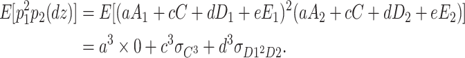
Figure 1 illustrates the path diagram in which all four factors are included. This is called the univariate ACDE model. In Fig. 1, p ₁ and p ₂ are phenotypes of the same trait for twin 1 and twin 2. In addition, let a, c, d, and e be the additive genetic effect, the shared environmental effect, the sum of the dominance effect and the interaction effect between genes (epistatic effect), and the nonshared environmental effect, respectively.

Fig. 1.

The ACDE model

To estimate a, c, d, and e, SEM using 2nd-order (and sometimes 1st-order) moments are used in current behavior genetic models (Eaves et al. 1978a, b; Neale and Carldon 1992). A significant problem in current behavior genetics models is that the ACDE model in Fig. 1 cannot be identified. Therefore, reduced ACE or ADE models are actually used in most research. However, the use of these reduced models may lead to biased estimators of these effects (Eaves et al. 1978a; Grayson 1989). The purpose of the present paper is to identify the ACDE model using non-normal structural equation modeling (nnSEM; Shimizu and Kano 2008; Ozaki and Ando 2009) to overcome this problem.

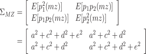
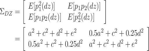
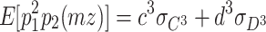
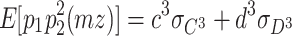
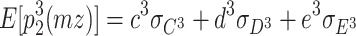
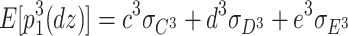
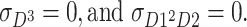
The reason why the ACDE model cannot be identified is as follows. The expected covariance matrices of the ACDE model for MZ and DZ twins are as follows:

1

2

Here, E[p ₁ p ₂(mz)] is the expectation of p ₁ p ₂ of MZ twins (here, let both p ₁ and p ₂ be mean centered phenotypes). The variances of A, C, D, and E are fixed to 1s. This model cannot be identified because there are three unique elements (one variance and two covariances). However, there are four parameters in the model (number of degrees of freedom: −1). Therefore, instead of the ACDE model, the ACE or ADE models are actually used.

In general, when twice the correlation between the DZ pair (r _dz) exceeds the correlation between the MZ pair (r _mz), the ACE model, in which D is removed, is used. Otherwise, the ADE model, in which C is removed, is used. In the latter case, MZ pairs are much similar than DZ pairs. Therefore, genetic effects are expected to be more important than common environmental effects, and d is included in the model. However, this model fit strategy is used because of the statistical limitation described above.

Actually, when twice the correlation between the DZ pair does not exceed the correlation between the MZ pair, this indicates only that the d effect is smaller than twice the c effect, because

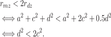Similarly when twice the correlation between the DZ pair exceeds the correlation between the MZ pair, the d effect is larger than twice the c effect. Keller et al. (2005) noted that r _mz > 2r _dz suggests only that c is less powerful than d, and not that c is non-existent.

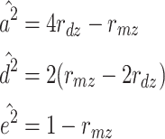
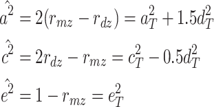
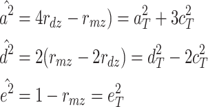
Including only three factors (ACE or ADE) often leads to incorrect results. Table 1 shows the biases in estimators (explained variance) for each factor when the ACE or ADE models are fit, even though all four factors actually affect a phenotype (which is realistic in most cases). The table shows that when the ACE model is fit, the explained variance for A is overestimated by 1.5d ², C is underestimated by 0.5d ², and D is underestimated by d ², and when ADE model is fit, A is overestimated by 3c ², C is underestimated by c ², and D is underestimated by 2c ² (as shown in the Appendix; see also Keller and Coventry 2005). In both the cases of the ACE and ADE models, the explained variance for E is estimated without bias. Therefore, both the ACE and ADE models yield biased estimators, except for E. In particular, C is underestimated whether the ACE model or the ADE model is fit. The constant results of small C effects in behavior genetics are to a degree due to the use of the ACE or ADE model (Grayson 1989).

Table 1.

Biases in estimators when the ACE model or the ADE model is fit

	ACE	ADE
	0	0

Subscript E denotes the estimator, and subscript T denotes the true value

Two numerical examples are given. First, in reality, if the explained percentage of variance for A, C, D, and E of a phenotype are all 0.25, then the MZ correlation is 0.75 (= 0.25 + 0.25 + 0.25) and the DZ correlation is 0.4375 (= 0.25 × 0.5 + 0.25 + 0.25 × 0.25). In this case, the ACE model is fit because r _mz < 2r _dz. Therefore, D is removed. However, in reality, D contributes as much as A, C, and E.

Second, when the explained variance for A, C, D, and E of a phenotype are 0.1, 0.2, 0.6, and 0.1, respectively, the MZ correlation is 0.9 (= 0.1 + 0.2 + 0.6), and the DZ correlation is 0.4 (= 0.1 × 0.5 + 0.2 + 0.6 × 0.25). In this case, the ADE model is fit because r _mz > 2r _dz. Therefore, C is removed. However, in reality, C has the second largest effect on a phenotype.

Table 1 and these two examples demonstrate that misspecification of the analysis model leads to incorrect results. In the present paper, in order to overcome this problem, the ACDE model is identified using nnSEM. The developed method provides more accurate estimators and is therefore the more accurate method for examining the etiology of variation in human behaviors. Eaves et al. (1978a) and Grayson (1989) noted that there are two primary problems in classical twin design, (which refers to behavior genetics research that uses only twin data and the ACE model or the ADE model is used), namely, (1) the inability to simultaneously estimate both C and D effects and (2) the inability to estimate higher-order epistasis effects. In addition, Keller and Coventry (2005) showed that problem (1) leads to larger bias in estimators than problem (2) (see also Coventry and Keller 2005). Therefore, although it does not perfectly explain variations in human behaviors, the ACDE model covers the primary behavioral factors.

nnSEM

The idea of using higher-order moments in SEM to accommodate non-normal variables was first suggested by Bentler (1983). Moreover, in 1985, a factor analysis model using non-normal variables and higher-order moments to eliminate rotational indeterminacy was developed by Mooijaart (1985). Therefore, the idea of using non-normal variables and higher-order moments is not a recent concept. However, Shimizu and Kano (2008) were the first to develop a simple regression model that uses non-normal variables and higher-order moments in the framework of SEM, where SEM using higher-order moments as well as (1st- and) 2nd-order moments is referred to as nnSEM. Also, Kano and Shimizu (2003) showed that using 2nd, 3rd, and 4th order moments a simple regression model considering confounding a latent variable can be identified.

And in the framework of Independent component analysis (ICA; Comon 1994), there are some researches using non-normally distributed disturbance variables. For example, Shimizu et al. (2006) showed that under the assumptions that the data generating process is linear, no confounding latent variable exists, and disturbance variables have non-normal distributions of non-zero variances, the best fit acyclic model can be identified. They called the model LiNGAM (a linear, non-gaussian, acyclic model). Hoyer et al. (2008) then showed that even if some confounding latent variables exist, parameter estimation of an acyclic model can be performed.

nnSEM has some advantages over SEM. For example, nnSEM can identify models that cannot be identified using SEM, because of a negative degree of freedom. Another advantage is that nnSEM can detect the direction of causation between two cross-sectional variables. Ozaki and Ando (2009) used this advantage to develop a method to detect the direction of causations between C factors and between E factors in bivariate behavior genetics models.

As an illustration of the former advantage, Toyoda (2007) showed that the spurious correlation model and the reciprocal causation model can be identified within the framework of nnSEM. The numbers of parameters of the spurious correlation model and the reciprocal causation model are both four (two path coefficients and two residual variances) when specifying models using only second-order moments. However, the number of unique elements of the covariance matrix between two variables is three. Therefore, neither the spurious correlation model nor the reciprocal causation model can be identified using SEM (number of degrees of freedom: −1). However, as shown in the Appendix of Ozaki and Ando (2009), nnSEM using second- and third-order moments can identify both models.

The two models can be identified using nnSEM because the use of third-order moments increases the number of moments of observed variables and therefore the number of degrees of freedom. Actually, the number of degrees of freedom of the spurious correlation model using nnSEM is 0 and that of the reciprocal causation model is 1. Therefore, these two models can be identified using nnSEM. In the present paper, using this advantage of nnSEM, the univariate ACDE model will be developed.

Model specifications

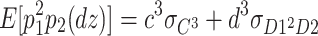
In addition to SEM using up to second-order moments, third-order moments are used in the present study. Sample third-order moments (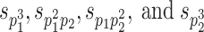) are calculated as follows when there are two phenotypes p ₁ and p ₂ (for twin 1 and twin 2, respectively):

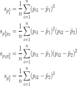where i indicates an observation (in this case, an observation pair). These sample statistics become information in the estimation of a, c, d, and e effects.

When three latent variables C, D, and E are assumed to follow non-normal distributions, the expected third-order moments for the MZ twins are as follows:

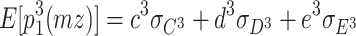3

4

5

6

In addition, the expected third-order moments for the DZ twins are as follows:

7

8

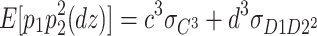9

10

Note that A is assumed to follow a normal distribution when many loci affect the phenotype of interest (Fisher 1918). Here, are the skewnesses of C, D, and E, respectively. (In this case, the variances of these independent factors are fixed to 1s. Therefore, these parameters are the skewnesses of the factors.) expresses the expected value of the second power of D of twin 1 times D of twin 2, and expresses the expected value of D of twin 1 times the second power of D of twin 2, respectively. and are assumed to be equal, because the order of twins is arbitrary.

The above equations are calculated as follows. For example,

Assumptions

However, the above model has not yet been identified. There are eight parameters () in the model. However, the number of unique equations is only six (three for second-order moments and three for third-order moments), resulting in the number of degrees of freedom being negative. Therefore, constraints are needed in order to identify the model. The following are models that can be identified.

1. C and E are non-normal, and D is normal. (Therefore, ) Furthermore, the skewnesses of C and E are the same () In this case, there are five parameters (and 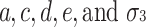), and the number of unique equations is five ( (Eq. 1) =  (Eq. 1) =  (Eq. 2) =  (Eq. 2), (Eq.1), 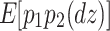(Eq. 2), (Eq. 3) =  (Eq. 6) =  (Eq. 7) =  (Eq. 10), and 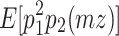(Eq. 4) =  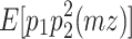(Eq. 5) =  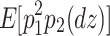(Eq. 8) =  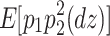(Eq. 9)), resulting in the number of degrees of freedom being 0. However, since there are 14 (six for second-order moments and eight for third-order moments) sample statistics and five parameters, the number of degrees of freedom used to calculate model fit indices is nine (=14 − 5). If the phenotypes are standardized, since the four variances are all 1s, the number of degrees of freedom is six (=11 − 5).

2. D and E are non-normal, and C is normal. (Therefore, Furthermore, the skewnesses of D and E are the same () and . In this case, there are six parameters (), and the number of unique equations is six, resulting in the number of degrees of freedom being 0. The number of degrees of freedom used to calculate model fit indices is eight (=14 − 6). If the phenotypes are standardized, then the number of degrees of freedom is five (=11 − 6).

3. D, C, and E are non-normal. Furthermore, the skewnesses of D, C, and E are the same (). In this case, there are six parameters (), and the number of unique equations is six, resulting in the number of degrees of freedom being 0. The number of degrees of freedom used to calculate model fit indices is eight (=14 − 6). If the phenotypes are standardized, then the number of degrees of freedom is five (=11 − 6).

Note that if all four latent factors are distributed normally, nnSEM cannot estimate these effects. The non-normal distributional assumption on D is likely. For example, if genotypes AA and Aa have the same effect on a trait and the gene frequencies of A and a are both 0.5, then D has a skewed distribution because the genotypic frequency of aa is 0.25 and the genotypic frequency of AA  +  Aa is 0.75. When researchers use the present method, they should compare the fits of the three identified models, and the results of the best fit model should be interpreted. An example R script can be downloaded from http://www.010.upp.so-net.ne.jp/koken/bg.html.

Note also that the developed ACDE model can be used only with continuous data and is not suitable for binary or ordinal data because, in order to analyze the latter two types of data, the liability model that assumes latent variables that follow some normal distributions is usually used in Behavior Genetics. However, if all four latent variables (A, C, D, and E) are normally distributed, then nnSEM cannot be used, because it is impossible to calculate the 3rd order moments of the assumed normally distributed latent variables.

Estimator

The asymptotically distribution-free (ADF) method (Browne 1982, 1984) is used to estimate parameters. In the two-group case (MZ and DZ), the ADF estimator can be expressed as follows:

11

Here, F is the function to be minimized, n is the sample size, σ(θ) is the expected second- and third-order moments vector, s is the observed second- and third-order moments vector, W is the weight matrix, and subscripts m and d denote MZ and DZ, respectively. Each element of W consists of n times the asymptotic covariance of estimators of moments of the observed phenotypes.

Simulation study

Settings

This simulation study examines the effects of two factors on the average biases and standard deviations of estimates of explained variance for A, C, D, and E. The two factors are (1) the true explained variance for A, C, D, and E (21 patterns, see Table 2), and (2) the skewness of C, D, and E (seven patterns, see Table 3). For all of the 147 (= 21 × 7) conditions, 300 replications were performed. Second- and third-order moments were used in the analyses. In each replication, the BICs of the three identified models are calculated, and the estimates of the best fit model were considered as the estimates in the replication. For the same generated data, when r _mz < 2r _dz, the ACE model was fit, otherwise the ADE model was fit. This enables comparisons between the results of the current method (SEM) and the developed method (nnSEM). The average biases and standard deviations of the estimates were calculated for each condition. In all cases, the numbers of MZs and DZs were both 600. The ADF estimator was used for both nnSEM and SEM analyses. For nnSEM, second- and third-order moments were used, on the other hand, for SEM only second-order moments were used. The analysis program was written using the R programming language (Ihaka and Gentleman 1996; version 2.4.0). We wrote the estimator, which was not a pre-existing R package. However, the ‘BFGS’ method, which is a quasi-Newton method, in the ‘optim’ function was used for optimization calculation.

Table 2.

True explained variances for A, C, D, and E

VC (nnSEM is true)				VC (nnSEM and SEM are true)
25	25	25	25	100/3	100/3	0	100/3
45	35	10	10	60	20	0	20
45	10	35	10	20	60	0	20
45	10	10	35	20	20	0	60
35	45	10	10	100/3	0	100/3	100/3
10	45	35	10	60	0	20	20
10	45	10	35	20	0	60	20
35	10	45	10	20	0	20	60
10	35	45	10
10	10	45	35
35	10	10	45
10	35	10	45
10	10	35	45

VC (nnSEM is true) denotes the conditions in which all four factors affect a trait. Therefore, nnSEM will be the appropriate method. On the other hand, VC (nnSEM and SEM are true) denotes the conditions in which ACE or ADE are the true models. Therefore, both nnSEM and SEM will be appropriate methods

Table 3.

Skewness of C–E

C	D	E	T/F
0	0	1	F
0	1	0	F
1	0	0	F
0	1	1	T
1	0	1	T
1	1	0	F
1	1	1	T

When the skewness is 0, the factor score was generated from the standard normal distribution. On the other hand, when the skewness is 1, the factor score was generated from the χ²(8) distribution. When one of the three models identified is the true model (patterns 4, 5, and 7), T/F is T and when none of the three models identified is the true model (patterns 1, 2, 3, 6, and 7), T/F is F

Twenty one patterns of the true explained variance were divided into two cases. In one case, all four factors affect a trait. Therefore, nnSEM is the true model. In the other case, three of the four factors (ACE or ADE) affect a trait. Therefore, both nnSEM and SEM are the true model. Figures 2 and 3 show the results for the former cases, and Figs. 4 and 5 show the results for the latter cases.

Fig. 2.

Biases (estimated value–true value) when all four factors affect a trait

Fig. 3.

Standard deviations of estimates when all four factors affect a trait

Fig. 4.

Biases (estimated value–true value) when three factors affect a trait

Fig. 5.

Standard deviations of estimates when three factors affect a trait

The seven patterns of skewness are shown in Table 3. These seven patterns can be divided into two cases, in which either (1) one of the three models identified is the true model (patterns 4, 5, and 7; denoted as T in Figs. 2, 3, 4, 5) or (2) none of the three models identified is the true model (patterns 1, 2, 3, and 6; denoted as F in Figs. 2, 3, 4, 5). In order to simplify the results, rather than seven patterns, the average of the results of the three T patterns and the average of the results of the four F patterns are presented in Figs. 2, 3, 4, 5. In all cases, the factor scores for A were generated from the standard normal distribution.

Results and discussion

Figures 2, 3, 4, 5 show the box plots for A, C, D, E, and G. Here, G indicates the results of A  +  D, which can be considered as the broad-sense heritability (Keller and Coventry 2005). In each figure, nnS indicates the case in which nnSEM was used for the analyses, and S indicates the case in which SEM was used. In addition, T and F in parentheses indicate whether one of the three models identified is the true model (T) or not (F). A, C, D, E, and G at the bottom of each figure indicate that the plots are the results for the corresponding factors. Figures 2 and 4 show the results for the average biases (estimated value–true value), and Figs. 3 and 5 show the results for the standard deviation of the estimates. The box plots are shown for the averages of the three T cases or the four F cases. For example, the box plot for A of the nnS(T) case in Fig. 2 was shown for the following values: 0.041, −0.060, −0.089, −0.145, −0.012, 0.031, 0.107, −0.080, 0.055, −0.016, −0.069, 0.098, and −0.004. The first value, 0.041, is the average of the 300 biases for A when using nnS(T) and the variance components for the four factors are the same (first case in Table 2). The results will be discussed based on (1) an examination of the estimation accuracy of the proposed method and (2) comparison of the estimation accuracies of the conventional method (SEM) and the proposed method (nnSEM).

Examination of estimation accuracy of the proposed method

The simulation study revealed the following characteristics of the proposed method. Note that the following interpretations are for T  +  F cases (T and F are pooled), except for point 11.

1. Figure 2 shows that when all four factors affect a trait, the explained variance of A tends to be slightly underestimated (−7.9% on average), and Fig. 3 shows that the average standard deviation of the estimates of the variance of A is 14.8% and occasionally exceeds 20%, which is a large value. Consequently, the variance of A is not accurately estimated under these conditions.

2. Figure 3 shows that the average standard deviation is larger in the T case (16.8%) than in the F case (12.8%). However, this does not mean that the F case yields better estimates than the T case, because the average bias is much smaller in the T case (−1.1%) than in the F case (−11.4%).

3. Figure 4 shows that when three of the four factors affect a trait, the explained variance of A tends to be somewhat underestimated (−19.5% on average), and Fig. 5 shows that the average standard deviation of the estimates of the variance of A is 10.8%, which is not a small value. Consequently, the variance of A is not accurately estimated under these conditions.

4. Figure 2 shows that when all of the four factors affect a trait, the biases of the explained variance of C are <5% in most cases and are at most 10.1%. Furthermore, Fig. 3 shows that the standard deviations of the estimates are <9%, which indicates that the variance of C is accurately estimated under these conditions.

5. Figure 4 shows that when three of the four factors affect a trait, the explained variance of C tends to be slightly overestimated (6.1% on average), and Fig. 5 shows that the average standard deviation of the estimates of the variance of C is 5.7%. Consequently, the variance of C is accurately estimated under these conditions.

6. Figure 2 shows that when all four factors affect a trait, the biases of the explained variance of D are <10% in most cases, and the explained variance of D tends to be overestimated. Figure 3 shows that standard deviation of the estimates is not larger than in the case of A. Consequently, the variance of D is not accurately estimated, but is estimated more accurately than the variance of A.

7. Figure 4 shows that when three of the four factors affect a trait, the biases of the explained variance of D are overestimated (12.0% on average). Figure 5 shows that the standard deviation of the estimates is not larger than in the case of A. Consequently, the variance of D is not accurately estimated, but is estimated more accurately than the variance of A. These results are the same as in the case in which all four factors affect a trait.

8. Figures 2, 3, 4, 5 show that whether three or four factors affect a trait, the biases of the explained variance of E are less than 5% in all cases. Furthermore, the standard deviations of the estimates are <5%, which indicates that the variance of E is very accurately estimated.

9. Figure 2 shows that when all four factors affect a trait, the biases of the average explained variance of G is −4%, and Fig. 3 shows that the standard deviations of the estimates are <10%.

10. Figure 4 shows that when all four factors affect a trait, the biases of the average explained variance of G is −7.5%, and Fig. 5 shows that the standard deviations of the estimates are <9%.

11. Figures 2, 3, 4, 5 show that whether three or four factors affect a trait, even if data is generated from a model that is not one of the three identified models (F cases), the results of biases and standard deviations of the estimates are not much larger than in the T cases, except for the biases for the A factor. This indicates that the proposed method can provide a similar level of accuracy for these two cases.

12. Figures 2, 3, 4, 5 show that if G = A + D is considered to be global effects of genes, then the explained variances of G, C, and E can be estimated accurately.

Comparison of the results obtained using SEM and nnSEM

The simulation study revealed the following characteristics. Note that the following interpretations are for T  +  F cases (T and F are pooled).

1. When all four factors affect a trait, for A, C, D, and G, there is a high probability of providing a smaller bias by nnSEM than by SEM under these conditions ((22/26) × 100 = 85% for A, (23/26) × 100 = 89% for C, (24/26) × 100 = 92% for D, and (21/26) × 100 = 81% for G).

2. In contrast, when three of the four factors affect a trait, for A, C, D, and G, SEM provided smaller biases than nnSEM in every case.

3. For E, both SEM and nnSEM provide very small bias whether three or four factors affect a trait.

4. The explained variance of C is always underestimated using SEM when all four factors affect a trait. However, this does not occur when using nnSEM.

5. SEM provides a smaller standard deviation of the estimates. Therefore, although nnSEM provides a smaller bias when all four factors affect a trait, a greater number of twins are needed in order to obtain the same level of standard deviation of the estimates using SEM.

Consequently, nnSEM was shown to provide better estimators than SEM in the cases in which four latent factors affect a trait. In particular, when G is considered as broad-sense heritability, G, C, and E can be estimated with biases of <5% in most cases for this simulation setting. When three latent factors affect a trait, SEM provides better estimators than nnSEM. However, even in these cases, C can be estimated with biases of <6.1% on average, E can be estimated with almost no bias, and G can be estimated with biases of <8% in most cases for this simulation setting using nnSEM.

Discussion

The ACE and ADE models yield biased estimates if the ACDE model is the true model. However, structural equation modeling cannot identify the ACDE model because of a negative degree of freedom. In the present paper, the ACDE model was developed using nnSEM. Simulation studies have suggested that the proposed method can decrease the biases and can be used even in cases in which three latent factors affect a trait if G, C, and E are used as outcomes. The effects of the MZ/DZ ratio on the results were not examined in the simulation study described above. However, a small simulation study was conducted, in which the cases of MZ:DZ = 800:400 and 400:800 were considered. The results showed that the MZ/DZ ratio has almost no effect on the estimates in this simulation setting.

In the present paper, although power calculation was not discussed, the power would be calculated by setting the true second- and third-order moments and analyzing the moments using a null model. This is the same method used to calculate the power in the SEM using Mx (Neale et al. 2006, p. 96).

There is another method of identifying the ACDE model. Kathryn et al. (2004) identified the ACDE model using sibling data, where one of the siblings is an adopted person, as well as twin data. Such sibling data also provides information of the etiology of human variation, because the siblings (one of whom is an adopted person) are thought to share the same environment, however, there is no genetic relationship between the siblings. Therefore, their similarity is thought to be caused by their shared environment. Unfortunately, gathering data for siblings for the case in which one sibling is adopted is very difficult and costly. In the present paper, however, nnSEM was used to identify the ACDE model in which higher-order moments are used as additional information. Since the method of the present paper can estimate a, c, d, and e effects using only twin data, the proposed method requires a much lower cost and is much easier to perform. Therefore, the proposed method contributes to behavior genetic research.

There are other factors that have possible effects on phenotypes, such as higher-order epistasis (Eaves et al. 1978a), assortative mating (people choose to marry persons similar to themselves; Eaves et al. 1984; Loelin and DeFries 1987), gene–environment correlation (Plomin et al. 1977; Eaves et al. 1977), and gene–environment interaction (Plomin et al. 1977; Eaves et al. 1977; Purcell 2002; Eaves and Erkanli 2003). The presence of higher-order epistasis makes the correlation between D factors of DZ twins lower than 0.25. The presence of assortative mating leads to overestimation of the effect of C and underestimation of the effect of A if these are not included in models. An example of gene–environment correlation is that genetically intellectual parents tend to provide an intellectual environment for their children, which in turn increases the intelligence of the children. The presence of positive gene–environment correlation also leads to overestimation of the effect of C and underestimation of the effect of A if these are not included in models. An extended twin-family design (ETFD, Truett et al. 1994) can estimate the effects of assortative mating and gene–environment correlation, but cannot estimate the higher-order epistatic effect or gene–environment interaction. Although Purcell (2002) proposed a relatively easy method of estimating gene–environment interaction, at present, there is no method that incorporates the higher-order epistatic effect in the model. Therefore, further research on developing a more exhaustive model is needed.

Higher-order epistasis is expressed as the correlation between D factors of DZ twins, and assortative mating is expressed as the correlation between A factors of DZ twins and D factors of DZ twins. gene–environment correlation is expressed as the correlation between A and C factors and between D and C factors, and gene–environment interaction is the interaction between one of the genetic factors and one of the environmental factors. Therefore, these four effects can be expressed as parameters associated with A, C, D, or E. Consequently, proper estimation of a, c, d, and e is an important basis for including these phenomena (such as assortative mating). Although, in the present paper, only the ACDE model was proposed, this is an important first step in the development of a more exhaustive model.

Appendix

When the ACE model is fit, the expected variance of a phenotype is a ² + c ² + e ², the expected correlation between MZs (r _mz) is a ² + c ², and the correlation between DZs (r _dz) is 0.5a ² + c ². Therefore, the simplest method of estimating a ², c ², and e ² when the ACE model is fit is as follows (when the phenotypes are standardized):

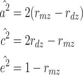When the ADE model is fit, the expected variance of a phenotype is a ² + c ² + d ², the expected correlation between MZs (r _mz) is a ² + d ², and the correlation between DZs (r _dz) is 0.5a ² + 0.25d ². Therefore, the simplest method of estimating a ², d ², and e ² when the ADE model is fit is as follows:

If the ACDE model is the true model and the true explained variances are respectively, then the expected correlation between MZs (r _mz) is and the expected correlation between DZs (r _dz) is 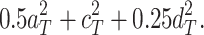Therefore, when the ACE model is fit, the estimators of the explained variances are as follows:

Therefore, and are biased ( and ).

When the ADE model is fit, the estimators of the explained variance are as follows:

Therefore, and are biased ( and ).

References

- Bentler PM. Some contributions to efficient statistics in structural models: specification and estimation of moment structures. Psychometrika. 1983;48:493–517. doi: 10.1007/BF02293875. [DOI] [Google Scholar]
- Bollen KA. Structural equations with latent variables. New York: Wiley; 1989. [Google Scholar]
- Browne MW (1982) Covariance structures. In: Hawkins DM (ed) Topics in applied multivariate analysis. Cambridge University Press, Cambridge, pp. 72–141
- Browne MW. Asymptotically distribution-free methods for the analysis of covariance structures. Br J Math Stat Psychol. 1984;9:665–672. doi: 10.1111/j.2044-8317.1984.tb00789.x. [DOI] [PubMed] [Google Scholar]
- Comon P. Independent component analysis—a new concept? Signal Process. 1994;36:287–314. doi: 10.1016/0165-1684(94)90029-9. [DOI] [Google Scholar]
- Coventry WL, Keller MC. Estimating the extent of parameter bias in the classical twin design: a comparison of parameter estimates from extended twin-family and classical twin designs. Twin Res Hum Genet. 2005;8:214–223. doi: 10.1375/twin.8.3.214. [DOI] [PubMed] [Google Scholar]
- Eaves JL, Erkanli A. Markov chain Monte Carlo approaches to analysis of genetic and environment components of human developmental change and G × E interaction. Behav Genet. 2003;33:279–299. doi: 10.1023/A:1023446524917. [DOI] [PubMed] [Google Scholar]
- Eaves LJ, Last KA, Martin NG, Jinks JL. A progressive approach to non-additivity and genotype–environmental covariance in the analysis of human differences. Br J Math Stat Psychol. 1977;30:1–42. [Google Scholar]
- Eaves LJ, Last KA, Young PA, Martin NG. Model-fitting approaches to the analysis of human behavior. Heredity. 1978;41:249–320. doi: 10.1038/hdy.1978.101. [DOI] [PubMed] [Google Scholar]
- Eaves LJ, Martin NG, Eysenck SBG. An application of the analysis of covariance structures to the psychogenetical study of impulsiveness. Br J Math Stat Psychol. 1978;30:185–197. [Google Scholar]
- Eaves LJ, Heath AC, Martin NG. A note on the generalized effects of assortative mating. Behav Genet. 1984;14:371–376. doi: 10.1007/BF01080048. [DOI] [PubMed] [Google Scholar]
- Fisher RA. The correlation between relatives on the supposition of Mendelian inheritance. Trans R Soc Edinb. 1918;52:399–433. [Google Scholar]
- Grayson DA. Twins reared together: minimizing shared environmental effects. Behav Genet. 1989;19:593–604. doi: 10.1007/BF01066256. [DOI] [PubMed] [Google Scholar]
- Hoyer PO, Shimizu S, Kerminen A, Palviainen M. Estimation of causal effects using linear non-gaussian causal models with hidden variables. Int J Approx Reason. 2008;49:362–378. doi: 10.1016/j.ijar.2008.02.006. [DOI] [Google Scholar]
- Ihaka R, Gentleman R (1996) R: a language for data analysis and graphics. J Comput Graph Stat 5:299–314. http://www.R-project.org
- Kano Y, Shimizu S (2003) Causal inference using nonnormality. In: Proceedings of international symposium on science of modeling—the 30th Anniversary of the Information Criterion (AIC), pp 261–270
- Kathryn AB-B, Kirby D-D, Thalia E, Jennifer JF, Jim S, Plomin R. A genetic analysis of individual differences in dissociative behaviors in childhood. J Child Psychol Psychiatry. 2004;45:522–532. doi: 10.1111/j.1469-7610.2004.00242.x. [DOI] [PubMed] [Google Scholar]
- Keller MC, Coventry WL. Quantifying and addressing parameter indeterminancy in the classical twin design. Twin Res Hum Genet. 2005;8:201–213. doi: 10.1375/twin.8.3.201. [DOI] [PubMed] [Google Scholar]
- Keller MC, Coventry WL, Heath AC, Martin NG. Widespread evidence for non-additive genetic variation in Cloninger’s and Eysenck’s personality dimensions using a twin plus sibling design. Behav Genet. 2005;35:707–721. doi: 10.1007/s10519-005-6041-7. [DOI] [PubMed] [Google Scholar]
- Loelin JC, DeFries JC. Genotype–environment correlation and IQ. Behav Genet. 1987;17:263–277. doi: 10.1007/BF01065506. [DOI] [PubMed] [Google Scholar]
- Mooijaart A. Factor analysis for non-normal variables. Psychometrika. 1985;50:323–342. doi: 10.1007/BF02294108. [DOI] [Google Scholar]
- Neale MC, Carldon LR. Methodology for genetic studies of twins and families. Dordrecht: Kluwer; 1992. [Google Scholar]
- Neale MC, Boker SM, Xie G, Maes HH. Mx: statistical modeling. 7. Richmond, VA: Virginia Commonwealth University, Department of Psychiatry; 2006. [Google Scholar]
- Ozaki K, Ando J. Direction of causation between shared and non-shared environmental factors. Behav Genet. 2009;39:321–336. doi: 10.1007/s10519-009-9257-0. [DOI] [PubMed] [Google Scholar]
- Plomin R, DeFries JC, Loehlin JC. Genotype–environment interaction and correlation in the analysis of human behavior. Psychol Bull. 1977;84:310–322. doi: 10.1037/0033-2909.84.2.309. [DOI] [PubMed] [Google Scholar]
- Purcell S. Variance components models for gene–environment interaction in twin analysis. Twin Res. 2002;5:554–571. doi: 10.1375/136905202762342026. [DOI] [PubMed] [Google Scholar]
- Shimizu S, Kano Y. Use of non-normality in structural equation modeling: application to direction of causation. J Stat Plan Inference. 2008;138:3483–3491. doi: 10.1016/j.jspi.2006.01.017. [DOI] [Google Scholar]
- Shimizu S, Hoyer PO, Hyvärinen A, Kerminen A. A linear non-gaussian acyclic model for causal discovery. J Mach Learn Res. 2006;7:2003–2030. [Google Scholar]
- Toyoda H. Theory of structural equation modeling. Tokyo: Asakura-shoten; 2007. [Google Scholar]
- Truett KR, Eaves LJ, Walters EE, Heath AC, Hewitt JK, Meyer JM, Siberg J, Neale MC, Martin NG, Kendler KS. A model system for analysis of family resemblance in extended kinships of twins. Behav Genet. 1994;24:35–49. doi: 10.1007/BF01067927. [DOI] [PubMed] [Google Scholar]