Neuronal Responses during and after the Presentation of Static Visual Stimuli in Macaque Primary Visual Cortex

Abstract

Viewing static visual scenes for several seconds or longer can induce a wide variety of striking percepts, including negative afterimages, fading, and motion aftereffects. To characterize the neuronal bases of such phenomena and elucidate functional circuitry in the visual system, we recorded responses of neurons in primary visual cortex (V1) of anesthetized macaques during and after the presentation of prolonged static visual stimuli. We found that 72% of cells generated significant after-responses (ARs) that outlasted classical off-transients after the cessation of stimuli, and AR amplitude grew with stimulus duration. After the longest stimuli tested (32 s), the amplitude and the time course of the AR were on average comparable to, and correlated with, those of the maintained response evoked while stimuli were present. These observations generally held regardless of cell class: simple, complex, direction selective (DS) or non-DS. The average decay time constant of the AR for orientation-tuned cells was 0.65 s. This is strikingly shorter than time constants observed in the lateral geniculate nucleus, which were on the order of tens of seconds. Cells in V1 that lacked orientation tuning displayed an intermediate time course, with a mean time constant of 4.3 s. These results are consistent with a multistage model in which cells at successive stages adapt to their inputs with progressively shorter time constants. Our findings suggest that the perceptual phenomena of fading and afterimages are shaped by both cortical and subcortical dynamics and provide a physiological framework for the interpretation of recent and long-standing psychophysical observations.

Introduction

Prolonged static visual stimuli have been essentially neglected in electrophysiological studies of the visual cortex, perhaps because they generate minimal or brief responses in most cortical cells (Emerson and Gerstein, 1977). In contrast, these same stimuli have given rise to a rich psychophysical literature because of the intriguing percepts that they generate, including fading (Ditchburn, 1973; Tulunay-Keesey, 1982; Burbeck and Kelly, 1984), negative afterimages (Kelly and Martinez-Uriegas, 1993; Wede and Francis, 2006), and motion aftereffects (Pierce, 1900; MacKay, 1957). Such psychophysical studies provide important clues to the operation of the visual system but suffer from the lack of a physiological basis for interpretation. For example, more than 100 years of study have not clarified whether afterimages arise from the retina or within the cortex (Delabarre, 1889; Creed and Harding, 1930; Misiak and Lozito, 1951; Loomis, 1972; Virsu and Laurinen, 1977; Shimojo et al., 2001; Gilroy and Blake, 2005; Tsuchiya and Koch, 2005).

We recently reported that lateral geniculate nucleus (LGN) neurons generate after-responses (ARs) with time constants of 10–100 s after static stimuli and that parvocellular (P) cells have ARs that are well matched in amplitude to their responses during stimuli, whereas magnocellular (M) cells have weaker ARs (McLelland et al., 2009). This raises two specific questions about ARs in primary visual cortex (V1). First, do V1 neurons maintain the long ARs from the LGN, or do responses decay quickly like the perception of afterimages, which may last only several seconds (Virsu and Laurinen, 1977; Kelly and Martinez-Uriegas, 1993)? Second, are the differences in the ARs of P- and M-cells maintained in the cortex or does convergence of these signals lead to a more complex pattern of results in V1 (Maunsell, 1987; Maunsell and Gibson, 1992)?

To address these questions, we studied responses in V1 during and after visual stimuli presented for 1–32 s at moderate luminance on a standard cathode ray tube (CRT) video display. We used the same stimuli as McLelland et al. (2009) to allow a direct comparison of LGN inputs to cortical responses. Within cortex, we divided cells into five physiological classes on the basis of orientation tuning, direction selectivity, and simple/complex receptive fields (RFs) (Hubel and Wiesel, 1962) to reveal any changes across the cortical hierarchy. For each cell class, we characterized the amplitude and time course of after-responses and compared this with stimulus-evoked responses. We examined the development of the AR with stimulus duration and compared it with that of the classical off-transient (OT) response. We present a simple model of sustained responses with multiple exponentially adapting stages that yields outputs consistent with our experimental results and sheds light on a recent psychophysical study (Tsuchiya and Koch, 2005) on the origin of afterimages. We also use our results to give a physiological account for the puzzling observation that streaming motion is perceived after the prolonged viewing of static, oriented gratings (Pierce, 1900; MacKay, 1957).

Materials and Methods

Subjects and surgery

Single-unit responses were recorded extracellularly from V1 (12 animals) and dorsal LGN (two animals) in anesthetized, paralyzed, rhesus macaques (Macaca mulatta). Before surgery, initial anesthesia was induced with ketamine HCl (10 mg/kg) and midazolam (0.10 mg/kg), followed by atropine sulfate (50 μg/kg). Anesthesia was maintained initially with isoflurane (0.5–2.0%) in a mixture of 50% O₂ and 50% room air while an endotracheal tube was inserted, the head was placed in a stereotaxic frame, a rectal thermometer was inserted, electrocardiogram (ECG) leads were attached, and cannulae were inserted into the saphenous veins in both legs. Anesthesia was then maintained with a combination of isoflurane (typically 0.25%) and sufentanil citrate (6–30 μg · kg⁻¹ · h⁻¹) in Hartmann's solution (3 ml · kg⁻¹ · h⁻¹) supplemented with dextrose (2.5%) and potassium (final concentration, 18 mmol/l). Artificial respiration, which commenced with the administration of sufentanil, was maintained with rate adjustments to keep expired CO₂ between 32 and 38 mmHg. Body temperature was maintained near 37°C with a heating pad. Sterile surgery consisted of a 13 mm trephine craniotomy followed by a small durotomy, placed over parafoveal opercular V1, ∼10 mm lateral to the midline and 4 mm posterior to the lunate sulcus, or for LGN, 11.5 mm lateral and 1–2 mm posterior to the central sulcus. EEG leads (typically eight channels) were placed on the cranium. A micromanipulator was placed so that the tips of the guide tubes containing electrodes were within 1 mm of the cortical surface (V1) or were inserted 2 mm into cortex (LGN), and a plastic chamber was placed around the guide tubes and filled with agar to stabilize pulsations of the cortex and to protect and seal the craniotomy. The agar was coated with petroleum jelly to prevent desiccation.

After surgery, paralysis was induced with vecuronium bromide (Norcuron; 0.1 mg · kg⁻¹ · h⁻¹) in Hartmann's solution (as above) to prevent movement of the eyes. The state of anesthesia was continuously monitored by EEG, ECG, and blood pressure (non-invasive), and the levels of sufentanil and isoflurane were adjusted as necessary. Daily maintenance of the animal included limb massage, injection of steroid (Solumedrone, 10 mg/kg) to minimize inflammation, and manual expression of the bladder (twice daily). Diapers were used to collect urine. The corneas were protected with gas-permeable hard contact lenses (+3 diopters), and supplemental lenses were added on the basis of direct ophthalmoscopy and were adjusted later to optimize neuronal responses to high spatial frequency visual stimuli. A reversing ophthalmoscope was used to plot the locations of the fovea on a flat-screen monitor directly in front of the animal.

A mechanical microdrive was used to advance quartz–platinum tungsten microelectrodes into the brain (Thomas Recordings). Electrodes were advanced vertically. Electrolytic lesions were made (50 μA at 12.5 kHz) on selected penetrations. At the end of the experiment, animals were given an overdose of sodium pentobarbital (65 mg/kg), exsanguinated through the heart with 0.9% saline, and perfused with 4% paraformaldehyde in saline. All procedures conformed to United Kingdom Home Office regulations on animal experimentation.

For histological verification of recording sites, the brain was blocked parasagittally, and blocks of tissue were cryoprotected by sinking in a series of sucrose solutions of increasing concentration (10–30%). Blocks were cut at 40 μm, mounted on slides, and stained for Nissl substance with cresyl violet. Electrode tracks were reconstructed by locating lesions and visualizing the damage to tissue caused by the electrodes.

It has been reported that isoflurane, compared with sufentanil, can reduce contrast sensitivity of some LGN neurons (Solomon et al., 1999), and although this study was different from ours in terms of animal (marmoset), visual stimulus (full-field illumination), and the combinations of anesthetic agents used, it is worth considering this issue. Unlike that study, we used isoflurane in the minimum amount needed to supplement sufentanil and this amount would not by itself induce anesthesia. In one animal, we used no isoflurane, and our results were not different. Having carried out many experiments under sufentanil alone in LGN and V1 (Bair et al., 2002; Bair and Movshon, 2004), we have noticed no difference in the physiological properties of either area when supplementary isoflurane is used. Also, the effects would be expected to be greatest at low contrast, whereas we used 100% contrast stimuli. Finally, our anesthetic protocol is consistent with our previous LGN experiments (McLelland et al., 2009).

Single-unit recording

Signals from the electrodes were amplified, bandpass filtered (0.5–2 kHz), played over an audio monitor, and digitized at 12.5 kHz using a standard analog-to-digital board (National Instruments) and custom software (C-code with Comedi drivers). Custom software was used for triggering and discriminating action potentials with multiple (typically one to three) time–amplitude windows. Electrodes were advanced until single-unit isolation was considered to be good on the basis of the presence of a refractory period and a clear separation between the accepted spikes and the rejected traces. Spike times were extracted at 1 ms resolution from the stored traces for additional analysis. The signal from a photodiode (Centronic OSD15-E) that sensed our visual stimulus display was digitized together with the electrode signals to accurately align spike times to the visual stimulus.

Visual stimuli

Basic characterization.

We first mapped cells by hand using bars and gratings while adjusting the depth of the electrode in micron increments to obtain a well-isolated action potential waveform. Hand mapping was performed on a 30-inch flat-screen monitor placed 50–80 cm from the eyes. For each cell, the dominant eye was determined on the basis of the audible responses to repeated stimuli, and the other eye was occluded. A front-silvered mirror was inserted to align the hand-mapped RF of the dominant eye onto the center of a 20 inch CRT (Eizo FlexScan F78, 96 Hz vertical refresh, 1024 × 768 pixels). The grayscale output of the monitor (27 cd/m² mean luminance) was linearized using a lookup table. We then characterized each cell physiologically under computer control using a series of drifting sinusoidal grating stimuli to generate tuning curves for direction of motion, spatial frequency (SF), temporal frequency (TF), and size. From the size tuning curve, we defined the optimal size, which we used for subsequent stimuli, to be the largest that yielded no less than the maximal response. We classified cells in V1 as simple or complex using a modulation index, MI = F1/DC, in response to an optimal drifting grating (Skottun et al., 1991), where DC is the mean evoked firing rate (in excess of the spontaneous rate), and F1 is the amplitude of the Fourier component of the response at the TF of the grating. We used a standard direction index, DI = 1 − a/p, to quantify the strength of DS, where p and a are the evoked firing rates for the preferred and anti-preferred direction of motion of drifting gratings (Maunsell and Van Essen, 1983).

For each neuron, we characterized the phase sensitivity by presenting static, optimal grating patches for 2 s at eight spatial phases equally spaced around one cycle. Interpolating the resulting tuning curves, we defined the preferred phase to be that which gave the highest firing rate during the stimulus and the anti-preferred phase to be 180° opposite (Fig. 1, stimulus icons). Thus, the preferred and anti-preferred stimuli were essentially photographic negatives. For simple cells (Fig. 1A), these stimuli caused responses with distinct time courses, but for complex cells (Fig. 1C) lacking any phase preference, the choice of the preferred phase was arbitrary.

Figure 1.

Phase sensitivity and response components of simple and complex cells to static stimuli. A, Raster plots show responses of a simple cell (orientation-tuned, non-DS) to six trials of a static sine grating presented for 2 s at the phase that drove the cell most strongly (top rasters) and at the phase 180° opposite (bottom rasters). The visual stimuli (icons shown to the right of the rasters) were optimized for orientation, size, and spatial frequency. Eight spatial phases were tested, but only two are shown here. The black-outlined stimulus was defined as the preferred for this cell, and the red-outlined stimulus was defined as the anti-preferred. B, PSTHs of the response to the preferred and anti-preferred stimuli. The preferred stimulus (black) evokes a visible transient “on” response, followed by an MR. The ending of the anti-preferred stimulus (red) evokes a transient “off” response, followed by a weak AR. C, D, Formatted as in A and B, responses are shown for a complex cell (orientation-tuned, non-DS), which by definition is insensitive to stimulus phase. The stimulus at each phase evokes a response with a similar time course that contains an on-transient, MR, off-transient and a weak or absent AR.

Static, variable duration.

We presented static preferred and anti-preferred stimuli for epochs having a variety of durations, followed by recovery epochs that tended to increase with the stimulus duration. The recovery epoch consisted of a flat gray screen at mean luminance. Specifically, a 2 s stimulus was followed by a 2 s recovery epoch, a 4 s stimulus by a 4 s recovery, 8 by 8, 16 by 8, and 32 by 16. The latter two recovery epochs were shorter than the stimulus epochs because experience showed that this was usually sufficient for firing rates in V1 to return to their spontaneous level. There was also a 1 s stimulus epoch followed by a 16 s recovery epoch to allow a direct comparison with the 16 s epoch after the longest (32 s) stimuli. This experimental design was intended to balance the need to allow the cell to recover between tests and the need to minimize the time to acquire multiple repeats of each condition.

Data analysis

Spontaneous firing rate for each cell was measured from intertrial periods during basic characterization, i.e., before prolonged adapting stimuli were presented. We typically used intertrial data from the characterization experiment that immediately preceded the prolonged adaptive stimuli, which was the test of phase sensitivity, for which intertrial periods were of 1 s duration, and firing rate during the last 200 ms of all intertrial periods was averaged (typically six repeats of eight phases).

To examine the time course of the response to static stimuli, we computed peristimulus time histograms (PSTHs) by averaging across spike trains time-locked to either the stimulus onset or stimulus offset. To attenuate noise, PSTHs were convolved with a Gaussian having an SD that was set depending on the timescale being studied (see Results). To estimate time constants, decaying exponential functions were fit to PSTHs.

We defined four response components that are evoked by static preferred and anti-preferred stimuli: a brief “on-transient” immediately after stimulus onset, a similar brief “off-transient” immediately after stimulus offset, a “maintained response” (MR) during the preferred stimulus, and a prolonged “after-response” that is visible after the off-transient. These four components are depicted by PSTHs in Figure 1 for a typical simple cell (Fig. 1B) and a typical complex cell (Fig. 1D). Simple cells, which by definition are phase sensitive, have positive-going on-transients and MRs in response to the preferred stimulus (black line) and positive-going off-transients and ARs in response to the anti-preferred stimulus (red line), whereas complex cells, defined to be phase insensitive, may have positive-going responses for all four components at all phases. We do not attempt to quantify negative-going responses, e.g., those that follow preferred stimuli in simple cells, because they are primarily hidden by truncation at zero firing rate, related to the low spontaneous rates of cortical neurons. When referring to the ARs, we will use subscripts, as in AR₃₂, to indicate the duration (here 32 s) of the stimulus that preceded the AR.

Modeling

We constructed a set of analytical models. Each model is built from one or more exponentially adapting units, as follows. The response, r(t), of each unit is equal to the scaled difference between the stimulus amplitude, s(t), and the reference adaptation level, a(t), plus a constant offset, b, equivalent to the baseline firing rate:

where c is a constant, and the adaptation level is given by

where * indicates convolution, and y(t) is a one-sided decaying exponential function:

Because r(t) represents the mean output firing rate, values <0 are set to 0.

For a single-stage model, s(t) took a value of 0 to represent zero contrast (blank gray) input, and −1 for the anti-preferred, suppressive stimulus. To model LGN P-cells, parameters were as follows: τ = 40 s, c = 40, b = 3.6 spikes/s (the latter value was taken from the average spontaneous firing rate of our P-cells). Similarly, to model cells in V1, parameters were as follows: τ = 1 s, c = 40, b = 2.3 spikes/s. The values of b and c are not critical here, except that b should have a positive value to allow a decrease in firing rate for suppressive stimuli.

For the two-stage model, the output of the first LGN-like stage was used as the input, s(t), to the second, V1-like stage. Parameters were as above, except that for the second stage, c = 1, because no additional scaling was required.

To model the psychophysical experiments of Tsuchiya and Koch (2005), we used a modified two-stage model in which the first stage comprised two adapting units in parallel, representing the monocular pathways at the level of the LGN, with parameters as above. These received different stimuli to reflect the dichoptic stimulus paradigm of their experiment. The input to the “left-eye” pathway represented the adapting stimulus for afterimage generation and took a value of −1, as above. The input to the “right-eye” pathway represented the masking stimulus, a flickering full-contrast Mondrian, and took a random value between −1 and 1 at each 100 ms interval, reflecting the fact that, for any individual cell in the LGN, this stimulus must sometimes be suppressive, sometimes excitatory. The second stage, representing the combination of the monocular pathways in V1, had V1 parameter values (above) and took the summed output of the monocular stages as its input. Stimulus trains lasted 30 s, alternating between zero contrast and the adapting stimulus/mask at 2 s intervals. The adapting stimulus and mask were present synchronously or asynchronously, or for comparison, no mask was included. See Tsuchiya and Koch (2005) for a fuller account of the stimulus paradigm.

Results

Our results are organized in five sections. Because ARs have not been characterized previously in visual cortex, we first present examples and provide a basic characterization of the amplitude and time course of these responses. We next compare ARs with MRs on a cell-by-cell basis. We then briefly examine the orientation dependence of ARs, and we compare ARs to classical off-transients. In the final section, we provide a simple model based on our findings and use it to interpret a recent psychophysical result.

Examples and basic characterization of after-responses

We recorded the MRs during, and the ARs after, prolonged static visual stimuli from 105 cells in V1, including 44 simple cells and 59 complex cells. Fourteen of the simple cells and 24 of the complex cells were direction selective (DS), and six of the simple cells had flat orientation tuning curves. We thus refer to five classes of cells: simple non-DS, simple DS, complex non-DS, complex DS, and untuned. The first four classes are orientation tuned, whereas the fifth lacks orientation tuning but is otherwise simple in nature, with tuning for SF, TF, and size. For the purpose of making direct comparisons betweenV1 and the LGN, we also report results for 19 P-cells and 14 M-cells, the responses of which have been partially described previously (McLelland et al., 2009).

Because perceptual afterimages depend on the duration of the adapting stimulus, we examined ARs using a paradigm in which the anti-preferred stimulus was presented for varying amounts of time. The spike train responses for this paradigm are shown in Figure 2 for two example simple cells and are aligned to the time at which the anti-preferred stimulus was extinguished. It is important to keep in mind that the low firing rate above the red bar (Fig. 2A) is associated with a suppressive stimulus, and the high firing rate thereafter is associated with a blank gray screen. After the shortest (1 s) anti-preferred stimulus, the first cell (Fig. 2A) elevated its rate for several seconds, and it fired much more after the longest (32 s) stimulus. The latter response, AR₃₂, was comparable in strength with the response to the preferred stimulus, i.e., the MR (Fig. 2B). This raises the possibility that such activity could be misinterpreted downstream as an indication that an oriented stimulus was present. In contrast, the second example cell (Fig. 2C) had a brief off-transient that was independent of stimulus length and had no AR, even for the longest stimulus. The response to the preferred stimulus (Fig. 2D) reveals that this cell was more transient than the first cell and had only a mild MR. Thus, some cells had strong ARs, and others had virtually none.

Figure 2.

Typical after-responses to prolonged static stimuli. A, C, Raster plots (10 trials each) of responses generated by two simple, non-DS cells after presentation of the anti-preferred stimulus for varying durations, aligned by stimulus offset time (16 and 32 s stimulus periods are truncated). B, D, Raster plots for the same cells as shown in A and C, respectively, showing the response during presentation of the preferred stimulus. Only 2 s of data are shown for D because this cell was never tested with a prolonged preferred stimulus as a result of the brevity of its responses. The cell shown in A generated a robust AR for all stimulus durations, with the duration and amplitude of the AR increasing in proportion to the stimulus. The AR₃₂ was greater in amplitude than the MR for this cell. In contrast, the cell shown in C generated only off-responses at all stimulus durations, never generating an AR. This was despite the cell showing some degree of MR.

To quantify the strength and time course of the mean AR for each cell, we computed PSTHs from the rasters aligned to stimulus offset. For each of the five physiological cell classes, Figure 3 shows PSTHs for four example cells that had the clearest ARs, sorted from top to bottom in approximate order of increasing AR duration. Cells with no AR are not shown here but are dealt with below. In each panel, AR₁ (blue line) and AR₃₂ (red line) are shown to assess whether the AR changed with stimulus duration, and the MR (black trace) is plotted for comparison. In some cases (e.g., Fig. 3A,C), we were unable to test responses to preferred stimuli of long duration, and for these cells we plot the MR for short (2 s) stimuli.

Figure 3.

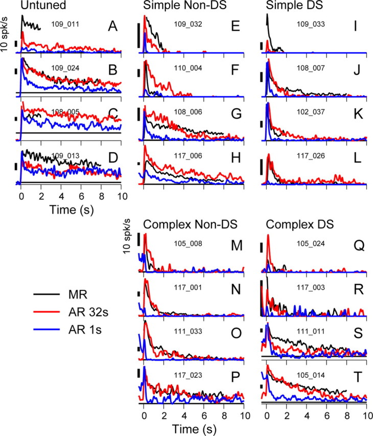
A sample of responses across cell classes. A–T, PSTHs (Gaussian smoothing, SD of 50 ms) for a selection of cells, grouped by cell class, showing AR₁ (blue), AR₃₂ (red), and MR (black). Horizontal black lines indicate spontaneous firing rates. Numbers in each panel indicate individual cell identities. The examples shown are selected from the cells showing the strongest AR in each class. Even so, variety in amplitude and duration of AR is apparent for all classes, except that the simple non-orientation-tuned class consistently shows a substantial and slowly decaying AR. Note that only the non-orientation-tuned cells did not include examples with minimal or no AR. Also note that the AR₃₂ could be smaller than (e.g., E and I), similar to (e.g., B and N), or larger than (e.g., F and Q) the MR.

Several key observations can be made on the basis of these examples and will be explored subsequently. First, the responses of the untuned cell class appeared to last longer than those of the orientation-tuned classes, and we observed only one short AR for this class; however, the group size was limited (n = 6). Each of the other classes included cells with strong ARs that decayed rapidly (Fig. 3E,I,M,Q) as well as cells with ARs that continued over many seconds (Fig. 3H,L,P,T). Each of these orientation-tuned classes also had cells that generated no significant AR (Table 1). Second, the AR₃₂ (red trace) was always at least as large as the AR₁ (blue trace) and usually substantially larger, suggesting that the AR typically grows with stimulus duration. Third, the AR₃₂ often resembled the MR in both amplitude and time course. Finally, substantial diversity of the response time course is apparent even among these examples of the strongest ARs in each cell class. Some are very brief, lasting <1 s, others go on for at least 10 s. We therefore applied a simple method to quantify the amplitude of the AR that could be applied to all cells: we took the mean firing rate in the 500 ms interval starting 150 ms after stimulus offset. This value, α_AR, reflects the early amplitude of the AR. The 150 ms delay was imposed to minimize the contribution from the off-transient. We accepted cells as having a significant after-response if α_AR for AR₃₂ was significantly greater than the spontaneous firing rate (t test, p < 0.05). In each cell class, ∼70–80% of cells qualified (Table 1).

Table 1.

AR and MR amplitude and time course

Cell class	Significant responses				Response amplitude (spikes/s)			Time constant (s)
	AR32		MR		AR1a	AR32a	MR	AR32	MR
Untuned	5 of 6	83%	6 of 6	100%	22.2 ± 20.2	36.5 ± 26.4	58.6 ± 22.4	4.3 ± 2.0	4.0 ± 1.4
Simple non-DS	18 of 24	75%	23 of 24	96%	9.1 ± 12.5	23.4 ± 23.6	26.3 ± 18.6	0.9 ± 2.4	1.3 ± 2.5
Simple DS	10 of 14	71%	9 of 14	64%	3.6 ± 3.7	10.8 ± 11.3	21.6 ± 22.6	0.9 ± 2.9	0.6 ± 1.9
Complex non-DS	24 of 35	69%	35 of 35	100%	7.1 ± 9.1	21.5 ± 18.6*	26.8 ± 20.1*	0.4 ± 2.6	0.8 ± 2.0
Complex DS	17 of 24	71%	21 of 24	88%	10.4 ± 14.8	22.6 ± 30.1	22.7 ± 28.5	0.6 ± 2.5	0.8 ± 2.8

The significant responses column indicates the fraction of cells that generated an α_AR (32 s stimulus) or α_MR significantly above the spontaneous firing rate of the cell (t test, p < 0.05). For response amplitude, mean ± SD of the α_AR and α_MR is shown.

^aComparing response amplitudes, the AR₃₂ was significantly larger than the AR₁ for all cell classes (Wilcoxon's signed-rank test, p < 0.05). Comparing AR₃₂ and MR, only the values with asterisks were significantly different (p < 0.005 Wilcoxon's signed-rank test; all other paired-mean comparisons for AR₃₂ vs MR had p > 0.05 for both Wilcoxon's signed-rank and paired t test). For time constants, the geometric mean ± SD is shown.

To investigate how the AR amplitude depends on stimulus duration, we considered only those cells having a significant AR. For each cell and stimulus duration, we computed α_AR, subtracted the spontaneous firing rate, and normalized all rates to the value for AR₃₂ before averaging across cells. The resulting plots for the orientation-tuned cell classes (Fig. 4, colored lines) show that α_AR for AR₃₂ was approximately three to four times larger than that for AR₁, and the increase is approximately proportional to the log of stimulus duration. Although this suggests that the AR could continue to grow with longer stimuli, the nature of this relationship means that exponentially increasing intervals will be required to yield substantial increases in response amplitude. By comparison, there was substantially less change in α_AR with duration for the untuned V1 cells (black line) and even less change for the LGN cells (gray lines). The relatively shallow slopes for these cell classes reflect a limitation in the stimulus paradigm that is best understood by considering the responses of LGN P-cells, which commonly have 10–100 s time courses (McLelland et al., 2009, their Fig. 4). Such cells build up their adaptation to the anti-preferred stimulus gradually over many trials and ultimately appear to respond to the absence of the anti-preferred stimulus as if it were the preferred stimulus. In this state, the response after a 1 s stimulus differs little from that after a longer stimulus, because the adaptation state of the cell does not change rapidly. Thus, the flatter slope of the V1 untuned cells in Figure 4 is consistent with their having longer adaptation time constants.

Figure 4.

Dependence of AR amplitude on stimulus duration. For each cell and each stimulus duration, the early AR firing rate was calculated. Spontaneous firing rate was subtracted, and values were normalized to the AR₃₂ value and then averaged across all cells of a given class. Only those cells having an AR₃₂ value significantly above their spontaneous firing rate were included (t test, p < 0.05). For the fraction of cells fulfilling this criterion, see Table 1.

Relationship of after-response to maintained response

Having observed that the AR amplitude increases with stimulus duration, we examined how the AR₃₂ related to the MR in terms of amplitude and time course. For amplitude, Figure 5A shows α_AR plotted against α_MR (defined similarly to the α_AR but for the MR) for all cells grouped by physiological cell class. Overall, α_AR and α_MR span the same range, from 0 to ∼100 spikes/s. These values were neither normally nor log-normally distributed for most cell classes (for statistical tests, see Fig. 5 legend). The correlation between α_AR and α_MR was strongest for the complex cells (Spearman's r = 0.90 and 0.88 for non-DS and DS cells, respectively). For DS complex cells, α_AR was not significantly different from α_MR, whereas it was on average slightly smaller for complex non-DS cells (for values, see Table 1). For simple cells, the correlation between α_AR and α_MR was weaker (r = 0.41 and 0.56 for non-DS and DS cells, respectively), and the means were not significantly different. Cells that had little or no AR₃₂ appeared in all classes and most of these also had a minimal MR (Fig. 5A, points clustered near the origin). Exceptions to this, i.e., cells with a strong MR and minimal AR₃₂, occurred only among simple cells (Fig. 5A, filled arrows) (see also Fig. 3E,I). The inverse, cells with an AR₃₂ much stronger than the MR, occurred only in the simple non-DS class (Fig. 5A, open arrow) (see also Fig. 3F). These cases of mismatched AR and MR amplitude account for the weaker correlations between α_AR and α_MR in the simple classes. These results hint at a greater functional diversity of simple cells compared with complex cells.

Figure 5.

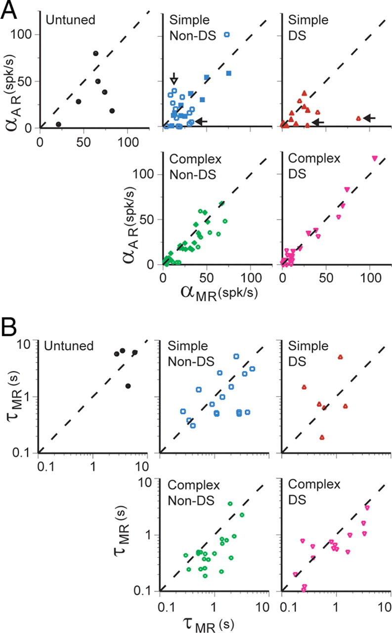
A, Relationship between amplitude of the early MR and AR₃₂, for individual cells, sorted by cell class. Mean spike rate was measured in a 500 ms window starting 150 ms after stimulus onset (MR) or offset (AR₃₂), thereby excluding the transient on- or off-response. Filled points indicate that there was no significant difference between MR and AR₃₂ amplitude. Distributions were neither normally nor log-normally distributed (Shapiro–Wilk test, p < 0.05) in the majority of cell classes. Spearman's correlation, r values: untuned, 0.20; simple non-DS, 0.41*; simple DS, 0.56*; complex non-DS, 0.90**; complex DS, 0.88** (*p < 0.05, correlation significant; **p < 0.001, correlation significant; values without asterisks were not significantly correlated, p > 0.05). B, Relationship between decay time constants of MR and AR₃₂ for individual cells, sorted by cell class. Decaying exponential curves were fit to PSTHs (bin size, 100 ms) from a start point 200 ms after the stimulus onset or offset, thereby excluding the transient on- or off-response. Only cells with AR₃₂ significantly above their spontaneous firing rate and that were adequately fit by decaying exponential functions are included. Raw data distributions failed the Shapiro–Wilk test for normality (p < 0.05) for all but the untuned class, but a logarithmic transform of the data yielded normal distributions throughout (Shapiro–Wilk test, p > 0.05 for both AR₃₂ and MR for each cell class). Hence, we have plotted the data on logarithmic axes. Pearson's correlation, r values for logarithmically transformed data points: untuned, −0.20; simple non-DS, 0.48; simple DS, 0.20; complex non-DS, 0.73**; complex DS, 0.80** (**p < 0.001, correlation significant; values without asterisks were not significantly correlated, p > 0.05).

To examine the relationship between the time course of the AR and MR in cells that had significant AR₃₂, we fit the responses with exponentially decaying functions (fits made to PSTHs from 0.2–16 s, bin width of 100 ms). Figure 5B shows the decay time constant of the AR₃₂ plotted against that of the MR. The data were judged to be log-normally distributed (see Fig. 5 legend); thus, we plot the data on logarithmic axes, and statistical comparisons are performed on the log-transformed data. Overall, time constants cover a range of ∼0.2–6 s (Table 1 shows geometric means of AR₃₂ and MR values). The sample of untuned cells, although small in number, falls at the longer end of this distribution (Fig. 5B, top left). The correlation of the AR and MR time constants was strong for complex cells (r = 0.73 and 0.80 for non-DS and DS, respectively; p < 0.001) but was not significant for simple cells (p = 0.48 and 0.20 for non-DS and DS, respectively). For complex non-DS cells, the AR₃₂ τ values were significantly less than those for the MR (paired t test, p < 0.001), but for all other cell classes, these values did not differ significantly (p > 0.05).

Overall, we find that the AR₃₂ tends to be positively correlated with the MR in terms of amplitude and time constant. Thus, cells with longer and stronger maintained responses during stimuli also have longer and stronger after-responses, although there are clear exceptions. Interestingly, complex cells show a tighter correlation, and simple cells have the striking exceptions. In the classical model of Hubel and Wiesel (1962), phase-insensitive complex cells are driven by a set of simple cells. If the output from, say, four simple cells with phase offsets drove a complex cell, it is likely that the MR from one simple cell would drive the complex cell MR, whereas the AR of a different (opposite phase) simple cell would drive the complex cell AR. However, then it should often occur that the AR and MR of complex cells differ, reflecting the diversity of response amplitude and time course across simple cells. On the contrary, the MR and AR of complex cells were significantly correlated. If complex cell time constants were consistently shorter than those of their presumed inputs, then this correlation could be explained by the shorter time constant dominating the response. However, it is clear that complex cells with long responses have well matched MR and AR (Figs. 3P,T, 5B). Alternatively, complex cells could receive input from many simple cells, such that the diversity in the inputs averages out. In this case, however, it is likely that complex cell responses would be less diverse than we observe. We can envisage three ways in which the matched MR and AR of complex cells might arise: (1) they take inputs selectively from orientation-tuned simple cells with matched time constants, (2) they receive significant input from cells with longer time constants (e.g., untuned V1 or LGN cells), allowing the relatively shorter time constant of the complex cell to dominate, or (3) ARs in complex cells are simply not directly derived from feedforward ARs. We currently cannot distinguish these possibilities.

To visualize the time course of ARs at the population level and to compare the time course across classes of cells within V1 and between V1 and LGN, we averaged together normalized PSTHs for AR₃₂ within each physiological class. For each cell with a significant AR, a PSTH (200 ms bin width) was computed, the spontaneous rate was subtracted, and all values were normalized to the first bin (taken to be 200–400 ms to exclude the off-transient). Normalized PSTHs were then averaged within cell classes and are shown in Figure 6A. The averages for the orientation-tuned cell classes (Fig. 6A, colored lines) have similar time courses that fall rapidly in the first 1 s and reach a plateau ∼4–8 s at ∼10% of the level in the first bin. This differs from the time course for the LGN P- and M-cells, which decay to ∼60% in the first 4 s. Despite the rapid initial decay of orientation-tuned responses, it appears that a sustained baseline is held that is above the spontaneous rate on average and lasts over the 16 s period of measurement. It is plausible that this baseline is supported by activity coming from the LGN input. The untuned cortical cells (Fig. 6A, black trace) show an intermediate behavior, initially lining up better with the LGN cells, but then dropping toward the level of the orientation-tuned cells by 16 s. These observations reinforce those from Figures 4 and 5B, that untuned cells have longer ARs than orientation-tuned cells, and it appears that there is a progressive shortening of the AR as signals pass from the LGN to untuned V1 cells and then to orientation-tuned V1 cells.

Figure 6.

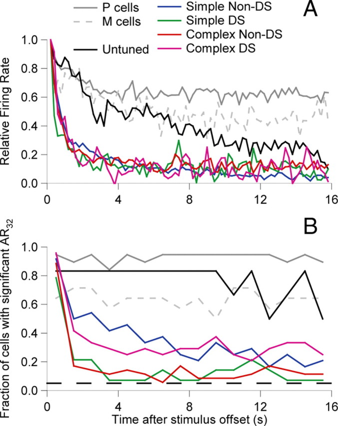
A, Population average PSTHs (bin size, 200 ms, no smoothing) for each cell class but including only those cells that did show an AR according to our standard criterion (firing rate significantly higher than spontaneous in the 500 ms period starting 150 ms after stimulus offset; n values as for Fig. 4). Before averaging, spontaneous rate was subtracted, and the values were normalized to the firing rate at the start of the after-response (200–600 ms). B, Normalized frequency histograms, showing the fraction of cells of each class with AR significantly above the spontaneous rate (p < 0.05) as a function of time. Significance tests were done for 1 s windows. The bottom dashed black line indicates the 5% significance level.

To estimate the fraction of the population that contributed to the AR as a function of time after the disappearance of the stimulus, we computed a frequency histogram of cells with firing rates significantly above their spontaneous rate (p < 0.05) as a function of time. To increase the power of the test, we used 1 s bins rather than the 200 ms bins above. As Figure 6B shows, in the first bin, the majority of cells had significant ARs (consistent with Table 1). For the LGN, the fraction of cells with a significant AR did not decay over the course of the 16 s studied here, remaining close to 93% for P-cells and 64% for M-cells. For untuned V1 cells, the pattern was similar, remaining constant at 83% up to 10 s but starting to decay beyond this point. For orientation-tuned cells, behavior was markedly different, with all classes showing a marked reduction in the fraction of cells showing a significant AR after only 1 s. This drop was somewhat less in simple non-DS cells (to 50%, followed by a gradual decay to ∼20% after 16 s) and in complex DS cells (to 42%, thereafter remaining relatively constant ∼29%) compared with simple DS and complex non-DS cells, which fell to ∼10% for the remaining period. In summary, two points worth emphasizing are that each physiological class contains cells with an AR₃₂ that lasts for a period of >10 s and that a large fraction of orientation-tuned cells show little if any AR after several seconds.

Orientation dependence of the after-response

So far, we have examined ARs in orientation-tuned cells in response to optimally oriented stimuli; however, there are two reasons to conduct a control with the static, adapting stimulus presented at another orientation. First, there is no fundamental reason why complex DS cells should fire an AR when a static stimulus is removed. These cells are defined as being sensitive to motion in a phase-independent manner; thus, neither a static stimulus nor a presumably static afterimage should drive these cells. (This differs from simple orientation-tuned cells, in which the negative afterimage of the anti-preferred stimulus would be a preferred stimulus.) It has been hypothesized that there is antagonism between static and movement channels (Georgeson, 1976); therefore, a static stimulus of any orientation might drive the AR of a complex DS cell on the assumption that there is a release from antagonism when the static stimulus disappears. Second, driven responses of non-DS orientation-tuned cells are known to be suppressed by cross-oriented stimuli (Morrone et al., 1982). It is therefore possible that there would be some release from suppression after removal of an orthogonal stimulus.

Conversely, there is a strong reason to suspect that the AR should be orientation tuned. Under what we will refer to as the hypothesis of “early equivalence,” ARs arise early in the system (e.g., in the retina) in cells that have spatially restricted RFs and that adapt to local luminance. A standing image would therefore fade to some degree, and, after its removal, the activity of the afferents would be equivalent to that caused by the presentation of the negative stimulus. Downstream orientation-tuned cells would then necessarily generate orientation-tuned responses (ARs). Also, the mere fact that we, and macaques (Schiller and Dolan, 1994), perceive patterned negative afterimages suggests that phase-sensitive cells in V1 should show some degree of selectivity. However, not all LGN cells live up to the principle of early equivalence (McLelland et al., 2009), and the far more rapid decay of ARs in V1 orientation-tuned cells raises the possibility that the cortical AR could involve its own mechanisms, including a nonselective response component.

We therefore tested a subset of cells with static gratings orthogonal to their preferred orientation. Figure 7A shows the MR and the AR₃₂ for an example complex cell at its preferred (top panel) and orthogonal (bottom panel) orientation. The AR₃₂ (red lines), which was strong for the preferred stimulus, is absent (not above spontaneous rate) for the orthogonal stimulus. For all cells tested (n = 11, including 7 DS), we plotted α_AR for orthogonal gratings against α_AR for preferred gratings (Fig. 7B). In all cases, the AR amplitude for orthogonal stimuli was lower than that for preferred stimuli.

Figure 7.

After-responses, like maintained responses, are orientation selective. A, PSTHs (Gaussian smoothing, SD of 50 ms) for an example complex DS cell (black line, MR; red line, AR₃₂). The top shows responses to the stimulus at the preferred orientation for the cell. The bottom shows the lack of response to the orthogonally oriented grating. B, α_AR for the orthogonally oriented stimulus versus α_AR for the stimulus at the preferred orientation for the cells tested (n = 11; upward pointing triangle, simple DS cell; downward pointing triangles, complex DS cells; diamonds, complex non-DS cells; dashed line indicates equality). Spontaneous firing rate has been subtracted from both values. The responses at the orthogonal orientation were always lower than those at the preferred orientation and in many cases not significantly above baseline.

We conclude that the AR is orientation tuned. The existence of an orientation-tuned AR is particularly interesting in complex DS cells because of a well-known visual illusion that has defied explanation: prolonged viewing of oriented lines leads to the perception of streaming motion orthogonal to the lines when the stimulus is removed. We will consider this issue further in Discussion.

The distinction between off-transients and after-responses

Our characterization of the AR has treated it as separate from the OT. We will not undertake a full characterization of OTs here, because they have received some attention in recent studies (Williams and Shapley, 2007; Huang et al., 2008), but it is worth considering what support there is for separating these two response components. We will focus on two questions: do OTs and ARs change with stimulus duration in a similar manner, and do they have similar variations across cell classes?

In Figure 8A–D, we have plotted poststimulus responses on a logarithmic timescale so that both the OT and slower response components are visible (see legend for methods). The PSTHs (Fig. 8A, top) of an example simple cell (that of Fig. 2C) show a substantial OT (red shaded band) that is similar after the 32 s stimulus (solid line) and the 1 s stimulus (dashed line). This would be highly uncharacteristic of an AR: all but 1 of 73 orientation-tuned cells that had a significant AR had an AR₃₂ of greater amplitude than the AR₁. Nonetheless, this lack of change in OT amplitude with stimulus duration was regularly observed and occurred in cells from each physiological class (Fig. 8C,D). The second example simple cell (Fig. 8A) shows a case in which the OT did grow with stimulus duration. The OT had a relatively long latency (peaking at ∼100 ms), and one could argue that this is part of the prominent AR (e.g., gray band) and that this cell has no true OT. However, the tendency of OTs to grow with stimulus duration was common (Fig. 8B) and could occur in cells having some of the earliest latency OTs. There were also examples of cells that had significant and strong ARs but in which the off-transients showed little dependence on duration (Fig. 8C,D, bottom panels). Thus, OTs show a range of behavior, but frequent examples of a lack of dependence on stimulus duration suggests that the OT may be distinct from the AR.

Figure 8.

The off-transient. A–D, PSTHs showing the off- and after-responses of eight example cells, two from each of the orientation-tuned cell classes, after the 1 s (gray dashed line) and 32 s (solid black line) stimuli. The time axis is logarithmic to enable simultaneous viewing of both the off-transient response and the AR. The width of the Gaussian kernel used to smooth traces was increased as a function of time, to maintain a degree of smoothing appropriate for the viewing resolution (specifically, we used SDs of 4, 16, and 64 ms to smooth the regions from ∼0–150, 150–500, and 500–9000, respectively). The precise boundaries were chosen as the closest points where the smooth segments intersected. The period over which we measured the amplitude of the off-transient (40 ms window starting at the half-rise point) is indicated by the red shaded area. For comparison, the window for measurement of the α_AR (fixed window from 150 to 650 ms) is indicated by the gray shaded area. E, Average off-transient amplitude (mean firing rate in the 40 ms after the half-rise point of the off-response) as a function of the stimulus duration. Responses for individual cells were normalized to the mean level for that cell before averaging across cells and then expressed relative to the response after the 32 s anti-preferred stimulus. F, Distribution of off-transient latencies (time to half-height after offset of 32 s anti-preferred stimulus) by cell class. Boxes indicate the range of the upper and lower quartiles, along with the mean value, and whiskers indicate the 10th and 90th percentiles.

To examine quantitatively how the OT grows with stimulus duration, we defined the OT amplitude to be the firing rate in the 40 ms window beginning at the half-rise point of the first peak in activity after stimulus offset (Fig. 8A–D, red bands). We also tested smaller fixed window intervals, or windows tailored to the width of the transient response in individual neurons, and found no qualitative difference in results. When no such peak was evident because there was minimal response or because activity rose very slowly, we set the window according to the equivalent latency of the on-transient, which is strongly correlated with (r = 0.84, p < 0.001) and not significantly different from (t test, p > 0.05) off-transient latency in cells that have both transients (data not shown).

Figure 8E shows cell class average curves for the dependence of OT amplitude on stimulus duration. For each cell, the amplitude at each stimulus duration was normalized to the mean amplitude across all durations. We then averaged this normalized data across cells within each class. Each class curve is plotted in Figure 8E relative to its value at 32 s. The LGN M-cells, which subjectively have a marked and discrete transient response, had an average OT amplitude (dashed gray line) that was independent of stimulus duration over the range of durations that we tested. In contrast, P-cell OT amplitude (solid gray line) increased linearly with the log of stimulus duration. In primary visual cortex, the trend for most cell classes resembled that of P-cells, with an approximately linear increase in OT amplitude with the log of stimulus duration. The result for untuned cells was noisy, and, given the limited size of this group, we have not attempted to interpret this result. Both classes of non-DS cells (simple and complex) displayed a strong increase in OT amplitude with stimulus duration, although the complex non-DS class response appears to be saturating at 16–32 s stimulus duration. Simple DS cells followed a generally similar trend except that the 1 s stimulus generated an unexpectedly strong response. Complex DS cells stand out because their OT amplitude, like that of M-cells, is independent of the stimulus duration. Subjectively, OTs in the complex DS class consistently comprised a more discrete, easily identifiable transient component than in the other cortical cell classes studied.

Could a strongly transient, fixed-amplitude OT in cortical cells be a signature of M-cell input? We found some evidence consistent with this in the distribution of OT latencies by cell class (Fig. 8F). Just as M-cell responses are consistently earlier than P-cell responses, complex DS cells responded earlier than the other cortical cells and earlier on average than P-cells. The range of latencies of simple DS cells included this early period but extended to longer latencies as well. Thus, it seems possible that DS complex cell OTs are M-driven.

Overall, we believe that differences in amplitude versus stimulus duration give additional support to the distinction between the AR and the OT, beyond the difference in timescale of these two response components. Furthermore, the distributions of OT latencies (Fig. 8F) suggest that our measurement of AR amplitude in the epoch starting at 150 ms should be primarily independent of the OT.

A model of after-response generation

To gain intuition about the way that ARs develop in cortex, we built a simple two-stage model with a slowly adapting LGN-like stage followed by a faster-adapting V1-like stage (see Materials and Methods). In particular, we wondered why cortical ARs continued to increase with stimulus durations (e.g., from 16 to 32 s) (Fig. 4) that were much longer than their AR time constants (<1 s).

We compared the output of the two-stage model with that of single exponentially adapting stages. For the single-stage model with a 40 s time constant (Fig. 9B), the AR decays slowly (Fig. 9B), and α_AR (Fig. 9E, dashed line) actually drops below AR₁ for short stimuli (e.g., 2 s) and grows modestly for longer stimuli. The counterintuitive decrease after short stimuli, with 1 s yielding a stronger response than 2 s, arises through the combination of long τ and the statistical properties of the stimulus. The 1 s stimulus is followed by a disproportionately long recovery period (16 s; see Materials and Methods) that, through random interleaving, can precede the other stimulus durations but only very rarely another 1 s stimulus. Thus, at the beginning of 1 s stimuli, on average, the adapted state is slightly higher than for other stimuli. This feature of the model is also apparent in the behavior of LGN P-cells (Fig. 4). Alternatively, for a fast single-stage model (τ = 1 s) (Fig. 9C), the increase in α_AR with the log of stimulus duration is strongly sublinear, with no change in amplitude apparent for stimuli longer than 8 s (Fig. 9E, dotted line), and is not consistent with the behavior of V1 cells (Fig. 4). However, in the two-stage model (Fig. 9D), in which the output of the LGN-like stage (τ = 40 s) drives the V1-like stage (τ = 1 s), the output of the second stage increases with stimulus duration over the whole stimulus range (Fig. 9E, solid line) but retains fast AR decay. This demonstrates that, because of the existence of slow adaptation at the LGN level, long time constants of adaptation need not be invoked at the cortical level to account for our results.

Figure 9.

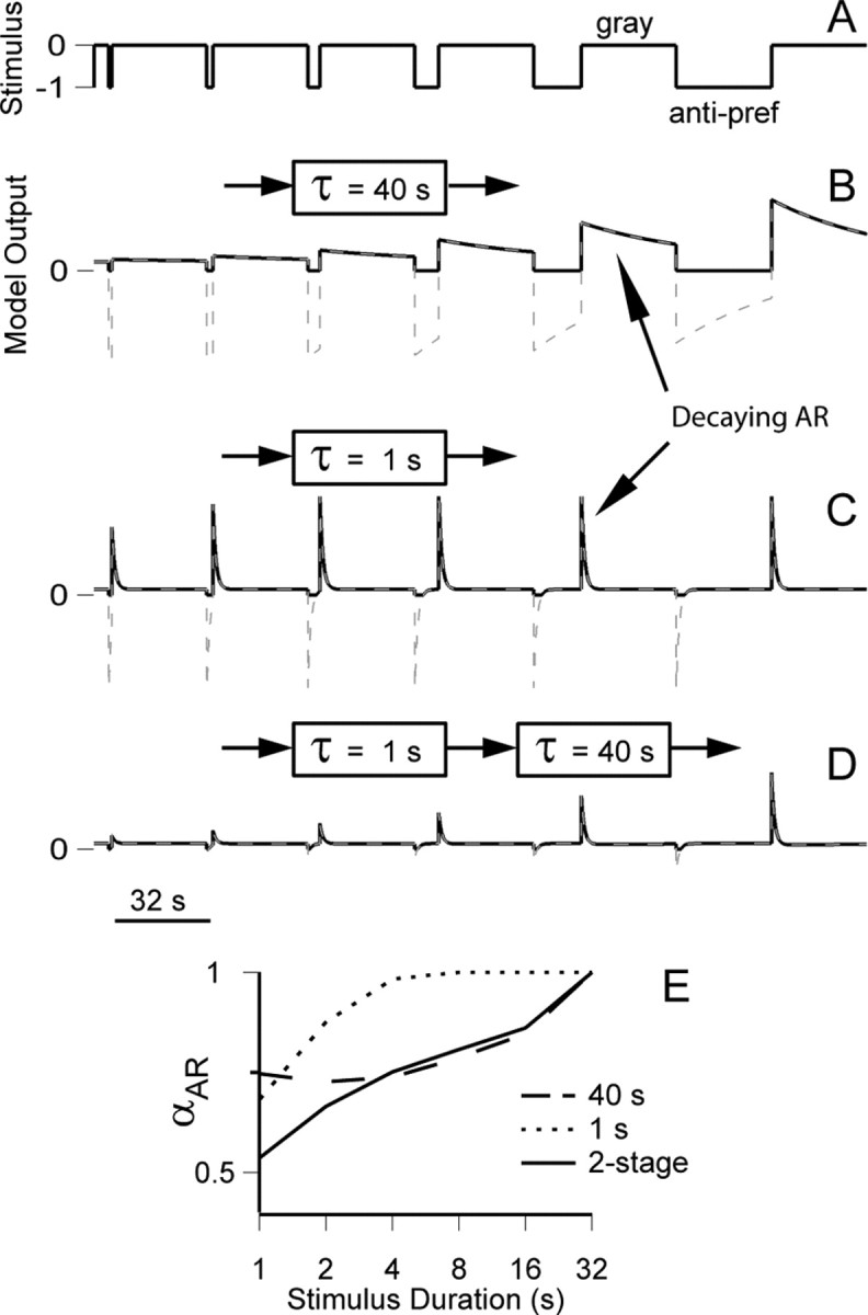
Model simulations of the buildup of AR amplitude with stimulus duration. A, The representation of the stimulus used in the model, switching from 0 (gray screen) to −1 (the anti-preferred stimulus). For clarity, the simulation shown here presents the adapting stimulus for sequentially increasing durations. B–D, The output of the model (dashed gray lines), zero-rectified to correspond to a firing rate (solid black lines). B, Single-stage exponentially adapting model, with τ = 40 s. C, Single-stage exponentially adapting model with τ = 1 s. D, Two-stage exponentially adapting model, with the output from the first stage (τ = 40 s) feeding into the second stage (τ = 1 s). E, Normalized AR amplitude as a function of stimulus duration for each of the three models, when tested with the same randomly interleaved stimulus used for in vivo experiments (6 blocks in each of which all stimulus durations were presented in random order; results here show the average of 10 such simulations).

Finally, we used the model to interpret the results of Tsuchiya and Koch (2005) who recently reported that dichoptic suppression of an adapting stimulus results in reduced afterimage strength. From this, they concluded that the formation of afterimages involves neural structures with input from both eyes, i.e., cortical neurons and suggested that higher-level processes were involved in suppressing the afterimage. However, this finding is entirely consistent with the behavior of our low-level binocular two-stage model (see Materials and Methods) given the linking hypothesis that ARs are related to afterimages. The model combines the output from two parallel, monocular LGN-like stages in a second V1-like stage. In the model, the left eye receives the adapting stimulus that would create an afterimage, and the right eye receives the stimulus that was intended to mask the afterimage. Although an AR develops normally in the former, the presence of excitatory activity in the latter reduces the AR developed at the cortical stage. Tsuchiya and Koch (2005) hypothesized that the diminished afterimage resulted from the consistency and completeness of the perceptual suppression in their paradigm rather than from a more direct effect of the masking stimulus on afterimage formation. To make this point, they used a paradigm in which the adapting stimulus and mask were turned on and off at 2 s intervals, either synchronously or asynchronously (Fig. 10B,C, left). They found afterimages to be reduced only in the synchronous case, i.e., when the adapting stimulus was perceptually masked. Our model reproduces these results but shows that they can arise through simple, direct pathways (Fig. 10). Importantly, the asynchronous condition always ended with 2 full seconds of the adapting stimulus with no mask. Because the time constant for cortical adaptation is short, with no mask present for the final 2 s of the stimulus train, there is almost no suppression of the cortical AR (Fig. 10C). In fact, our model predicts that ARs, thus afterimages, would be reduced even if the masking stimulus was presented only for the last few seconds of the adapting period. We conclude that an explicit model, including knowledge of the underlying signals, can be useful for interpreting psychophysics.

Figure 10.

Simulation of a psychophysical experiment (Tsuchiya and Koch, 2005). The model used has three exponentially adapting stages: the first two in parallel, representing P-cells in the right and left LGN, both with τ = 40 s; and the third, taking as input the combined output of the first two stages, representing V1, with τ = 1 s. Stimulus representation (left column; each box or space has 2 s duration), responses in the LGN (central column) and in V1 (right column). The inset shows a higher-resolution comparison of the after-responses generated in the V1 stage at the end of the stimulation period. A, Analogous to the psychophysical experiment, with no mask, an after-response develops in V1. B, When a dichoptic mask is presented synchronously with the adapting stimulus, the buildup of the V1 after-response is somewhat suppressed. C, When the mask is presented asynchronously to the adapting stimulus, because the stimulus period ends with two seconds of adaptation and no mask, and the V1 time constant is relatively short (1 s), the V1 after-response is almost no different from that which develops in the absence of the mask (traces for the no mask and asynchronous mask conditions nearly superimpose).

Discussion

Our characterization of V1 responses during and after the presentation of prolonged static visual stimuli has yielded several key findings. (1) The majority of cells in each physiological cell class, and 72% overall, had a significant AR, which increased in amplitude with stimulus duration. (2) AR amplitude and time course correlated with those of the MR. (3) Many DS cells had substantial ARs, suggesting a substrate for motion aftereffects. (4) ARs decayed much faster in orientation-tuned V1 cells than they did in LGN cells. (5) The AR and off-transient can be viewed as distinct response components, although they may overlap in time. We also presented a simple two-stage model as a starting point for interpreting psychophysical experiments under the linking hypothesis that afterimages arise from cortical ARs.

Transformation from LGN to V1

Comparing after-responses in V1 with those in LGN (McLelland et al., 2009) reveals two major differences. First, the decay time constant τ shortens from 10–100 s in LGN to 0.65 s on average for orientation-tuned V1 cells. Interestingly, V1 cells lacking orientation tuning had intermediate values of τ, mean of 4.3 s, raising the possibility that orientation selectivity is associated with a particularly rapid adaptation mechanism. Our untuned cells might represent an intermediate step between the LGN and the V1 output, given that a lack of orientation tuning is associated with layer 4C (Blasdel and Fitzpatrick, 1984; Hawken and Parker, 1984; Snodderly and Gur, 1995) and that these cells were all encountered near the middle of runs of highly active gray matter, a feature consistent with geniculo-recipient layers (Snodderly and Gur, 1995). The second major difference relates to our previous finding that M-cell ARs were weaker than their MRs, whereas P-cell ARs and MRs had similar amplitude. There was no such dichotomy in V1: none of the cell classes showed M-like behavior, although there were individual examples of this among simple cells. Unexpectedly, the DS complex cells, most tightly linked to the M-pathway (Livingstone and Hubel, 1988; Merigan and Maunsell, 1993; Movshon and Newsome, 1996; Yabuta and Callaway, 1998; Sincich and Horton, 2005), had the best match in MR and AR amplitude among all cell classes. This calls into question the role of M-cell MRs and ARs in driving V1 responses and presents a particular challenge to models in which DS responses are driven solely from M-inputs. However, off-transients in complex DS cells shared M-cell characteristics, occurring early and having an amplitude that was independent of stimulus duration.

To capture the most salient features of the transformation from LGN to V1, we proposed a simple two-stage model with slow subcortical adaptation followed by fast adaptation in V1. This model reframes the debate as to whether afterimages (if they are based on ARs) arise in or before the cortex. If signals from the retina and LGN were non-adapting, then cortical neurons could nonetheless generate after-responses (Fig. 9B). However, we know that signals from the LGN adapt strongly and thus do contribute to the after-response in the cortex. Inevitably, to understand the response at the end point, the whole system must be considered. Ultimately, the answer may be that afterimages arise from both the retina and V1, and there is no reason to assume that this does not extend to adaptation in extrastriate cortex (Kohn, 2007).

Mechanisms of cortical adaptation

Is the transformation observed from LGN to V1 consistent with known mechanisms of adaptation in V1?

Relative to the form of adaptation studied here, considerable attention has been given to contrast (or pattern) adaptation, whereby prolonged presentation of high-contrast moving stimuli, typically drifting gratings, leads to an elevation in contrast thresholds for similar patterns (Blakemore and Campbell, 1969; Graham, 1989). In neurons, this causes deformations of tuning curves for orientation, direction, and SF (Maffei et al., 1973; Movshon and Lennie, 1979; Albrecht et al., 1984; Bonds, 1991; Kohn, 2007).

It is likely that contrast adaptation is distinct from the adaptation to static stimuli that we studied here, as follows. Our static stimuli can cause response changes that are opposite to those of contrast adaptation: prolonged presentation of a high contrast (anti-preferred) stimulus greatly enhances the response during low (zero) contrast illumination, i.e., the gray screen in the absence of a stimulus. Furthermore, contrast adaptation uses dynamic stimuli that drive V1 neurons continuously at high firing rates, engaging mechanisms that are not likely to be engaged by the relatively weak cortical responses to static stimuli. Finally, at the level of the retina and LGN, Solomon et al. (2004) showed that contrast adaptation was restricted to the M-pathway, whereas we found strong static adaptation in the P-pathway, with postsuppression after-responses weak or absent in the M-pathway (McLelland et al., 2009).

At the cellular or circuit level, several adaptive mechanisms are recognized in cortex (Kohn, 2007). It has been shown that contrast adaptation is mediated by the activation of hyperpolarizing currents in the adapting cell (Carandini and Ferster, 1997). In cat cortex, contrast adaptation and intracellular current injection have similar hyperpolarizing effects (Sanchez-Vives et al., 2000), but these last ∼4.5 s (Albrecht et al., 1984), which is longer than what we observed in orientation-tuned V1 cells (<1 s). This difference might relate to the sinusoidal input modulation of these stimuli; however, postadaptation suppression from contrast adaptation, a period exempt from sinusoidal modulation, was even longer, on the order of 20 s (Sanchez-Vives et al., 2000).

A second mechanism proposed to underlie adaptation in V1 is synaptic depression (Abbott et al., 1997; Chance et al., 1998). Although mostly characterized in vitro (Stratford et al., 1996; Abbott et al., 1997), recently Chung et al. (2002), recording in the rat somatosensory cortex in vivo, concluded that synaptic depression rather than postsynaptic somatic mechanisms accounted for firing rate adaptation. Interestingly, time constants of adaptation were on the order of 0.25 s for depression and 4 s for recovery, closer to the range that we observed here than the intracellular mechanisms associated with contrast adaptation. Intracellular studies of visual neurons during prolonged static adaptation are probably required to shed light on the underlying mechanisms.

Regardless of the mechanism by which orientation-tuned cells diminish responses to static stimuli, the phenomenon is consistent with theories about adaptation for redundancy reduction (Barlow, 1972) and signal separation for the improvement of signal-to-noise ratios (Barlow, 2001). In particular, our data reflect a diversity of response decay time constants that could serve to emphasize the different TF components of dynamic stimuli. Another possible function is reducing metabolic demands associated with spiking (Levy and Baxter, 1996; Lennie, 2003).

Relation to psychophysical studies

Given that ARs in V1 can be, for most cells, as strong as MRs, we believe that it is reasonable to posit that ARs could underlie the perception of afterimages, just as it is generally hypothesized that driven responses underlie the perception of actual visual stimuli. General experience suggests that our perception of static images is fleeting. In particular, visual fading occurs within several seconds (Ditchburn, 1973; Tulunay-Keesey, 1982) and afterimages decay on a similar timescale (Virsu and Laurinen, 1977; Kelly and Martinez-Uriegas, 1993). These time courses are substantially shorter than those of ARs in LGN but are covered by the range of time constants observed in V1. Only Kelly and Martinez-Uriegas (1993) investigated the time course of afterimages using a stimulus like ours, i.e., static sinusoidal gratings at nonbleaching luminance levels. They found afterimage amplitude to build up and decay with an exponential time course, with τ on the order of 4–8 s, which is longer than our average V1 decay time. There are several possible explanations for this difference. First, they used a cancellation paradigm to estimate the afterimage time course. When we simulated this (data not shown) in our two-stage model, we found that the cancellation paradigm need not identify the time constant of adaptation in the final, fastest stage but rather can be influenced by multiple stages. In short, the time course estimated by Kelly and Martinez-Uriegas is not inconsistent with slightly shorter time courses in V1. Second, all classes of orientation-tuned V1 cells contained some neurons with time constants on the order of several seconds. Finally, the untuned V1 neurons, rather than simply being an intermediate step to orientation tuning, could represent a pathway encoding color and luminance (Livingstone and Hubel, 1988) that is important for the perception of afterimages.

It is striking that many DS cells, especially complex cells, generated strong and relatively sustained MRs and ARs to static stimuli. Complex DS cells project to visual cortical area V5/middle temporal area MT (Movshon and Newsome, 1996), which plays an important role in motion perception (Britten et al., 1992; Salzman et al., 1992). This raises the question of whether ARs in such cells lead to motion aftereffects. This seems as reasonable to ask as whether ARs of simple cells underlie negative afterimages. It has long been known that the prolonged viewing of static, oriented gratings leads afterward to the perception of motion that streams orthogonal to the adapting orientation (Pierce, 1900; MacKay, 1957). We speculate that this percept reflects the downstream consequences of the activity observed here in DS cells. We verified that DS cells, which are orientation tuned, have ARs that are also orientation specific. This offers an explanation of why the illusory motion only runs orthogonal to the adapting orientation: because DS cells prefer motion orthogonal to their preferred orientation (Hubel and Wiesel, 1968; Albright, 1984). This differs from past explanations that called on competitive cross-orientation interactions (MacKay, 1957; Kim and Francis, 2000). If this is the case, and given that the MR matched the AR in these cells, this raises the question of why the illusory motion is not perceived during the viewing of the static stimulus itself. A possible solution comes from Georgeson (1976) (MacKay and MacKay, 1976), who hypothesized that there is competition between static and motion channels, which allows the static channel to win while the stimulus is present, and the motion signals to dominate when the stimulus disappears. This, however, would require the added hypothesis that the static channel is more strongly activated by true stimuli than by afterimages. This suggests that activity in the LGN–M pathway, which is stronger during stimuli than afterward (McLelland et al., 2009), may play an important role in the static pathway. Additional studies will be required to understand how the signals available in V1 influence responses in higher areas, such as V5/MT, that may be relevant for the perception of this illusory motion.

We have attempted to demonstrate that an electrophysiological characterization of after-responses and a simple model based on the experimental data can be useful for interpreting psychophysical findings. This might extend to other features of afterimages. For example, the combination of long and short time constants in series could help to explain our ability to “refresh” an afterimage by blinking, after it has faded perceptually. This may require more elaborate models that include the M-cell signals.

References

- Abbott LF, Varela JA, Sen K, Nelson SB. Synaptic depression and cortical gain control. Science. 1997;275:220–224. doi: 10.1126/science.275.5297.221. [DOI] [PubMed] [Google Scholar]
- Albrecht DG, Farrar SB, Hamilton DB. Spatial contrast adaptation characteristics of neurones recorded in the cat's visual cortex. J Physiol. 1984;347:713–739. doi: 10.1113/jphysiol.1984.sp015092. [DOI] [PMC free article] [PubMed] [Google Scholar]
- Albright TD. Direction and orientation selectivity of neurons in visual area MT of the macaque. J Neurophysiol. 1984;52:1106–1130. doi: 10.1152/jn.1984.52.6.1106. [DOI] [PubMed] [Google Scholar]
- Bair W, Movshon JA. Adaptive temporal integration of motion in direction-selective cells in macaque visual cortex. J Neurosci. 2004;24:7305–7323. doi: 10.1523/JNEUROSCI.0554-04.2004. [DOI] [PMC free article] [PubMed] [Google Scholar]
- Bair W, Cavanaugh JR, Smith MA, Movshon JA. The timing of response onset and offset in macaque visual neurons. J Neurosci. 2002;22:3189–3205. doi: 10.1523/JNEUROSCI.22-08-03189.2002. [DOI] [PMC free article] [PubMed] [Google Scholar]
- Barlow HB. Single units and sensation: a neuron doctrine for perceptual psychology? Perception. 1972;1:371–394. doi: 10.1068/p010371. [DOI] [PubMed] [Google Scholar]
- Barlow HB. Redundancy reduction revisited. Network Comput Neural Syst. 2001;12:241–253. [PubMed] [Google Scholar]
- Blakemore C, Campbell FW. On the existence of neurones in the human visual system selectively sensitive to the orientation and size of retinal images. J Physiol. 1969;203:237–260. doi: 10.1113/jphysiol.1969.sp008862. [DOI] [PMC free article] [PubMed] [Google Scholar]
- Blasdel GG, Fitzpatrick D. Physiological organization of layer 4 in macaque striate cortex. J Neurosci. 1984;4:880–895. doi: 10.1523/JNEUROSCI.04-03-00880.1984. [DOI] [PMC free article] [PubMed] [Google Scholar]
- Bonds AB. Temporal dynamics of contrast gain in single cells of the cat striate cortex. Vis Neurosci. 1991;6:239–255. doi: 10.1017/s0952523800006258. [DOI] [PubMed] [Google Scholar]
- Britten KH, Shadlen MN, Newsome WT, Movshon JA. The analysis of visual motion: a comparison of neuronal and psychophysical performance. J Neurosci. 1992;12:4745–4765. doi: 10.1523/JNEUROSCI.12-12-04745.1992. [DOI] [PMC free article] [PubMed] [Google Scholar]
- Burbeck CA, Kelly DH. Role of local adaptation in the fading of stabilized images. J Opt Soc Am A. 1984;1:216–220. doi: 10.1364/josaa.1.000216. [DOI] [PubMed] [Google Scholar]
- Carandini M, Ferster D. A tonic hyperpolarization underlying contrast adaptation in cat visual cortex. Science. 1997;276:949–952. doi: 10.1126/science.276.5314.949. [DOI] [PubMed] [Google Scholar]
- Chance FS, Nelson SB, Abbott LF. Synaptic depression and the temporal response characteristics of V1 cells. J Neurosci. 1998;18:4785–4799. doi: 10.1523/JNEUROSCI.18-12-04785.1998. [DOI] [PMC free article] [PubMed] [Google Scholar]
- Chung S, Li X, Nelson SB. Short-term depression at thalamocortical synapses contributes to rapid adaptation of cortical sensory responses in vivo. Neuron. 2002;34:437–446. doi: 10.1016/s0896-6273(02)00659-1. [DOI] [PubMed] [Google Scholar]
- Creed RS, Harding RD. Latency of after-images and interaction between the two retino-cerebral apparatuses in man. J Physiol. 1930;69:423–441. doi: 10.1113/jphysiol.1930.sp002661. [DOI] [PMC free article] [PubMed] [Google Scholar]
- Delabarre EB. On the seat of optical after-images. Am J Psychol. 1889;2:326–328. [Google Scholar]
- Ditchburn RW. Eye movements and visual perception. Oxford: Clarendon; 1973. [Google Scholar]
- Emerson RC, Gerstein GL. Simple striate neurons in the cat. I. Comparison of responses to moving and stationary stimuli. J Neurophysiol. 1977;40:119–135. doi: 10.1152/jn.1977.40.1.119. [DOI] [PubMed] [Google Scholar]
- Georgeson M. Antagonism between channels for pattern and movement in human vision. Nature. 1976;259:413–415. doi: 10.1038/259413a0. [DOI] [PubMed] [Google Scholar]
- Gilroy LA, Blake R. The interaction between binocular rivalry and negative afterimages. Curr Biol. 2005;15:1740–1744. doi: 10.1016/j.cub.2005.08.045. [DOI] [PubMed] [Google Scholar]
- Graham N. Visual pattern analyzers. New York: Oxford UP; 1989. [Google Scholar]
- Hawken MJ, Parker AJ. Contrast sensitivity and orientation selectivity in lamina IV of the striate cortex of Old World monkeys. Exp Brain Res. 1984;54:367–372. doi: 10.1007/BF00236238. [DOI] [PubMed] [Google Scholar]
- Huang X, Levine S, Paradiso MA. Rebounding V1 activity and a new visual aftereffect. J Vis. 2008;8:1–10. doi: 10.1167/8.3.25. [DOI] [PMC free article] [PubMed] [Google Scholar]
- Hubel DH, Wiesel TN. Receptive fields, binocular interaction and functional architecture in the cat's visual cortex. J Physiol. 1962;160:106–154. doi: 10.1113/jphysiol.1962.sp006837. [DOI] [PMC free article] [PubMed] [Google Scholar]
- Hubel DH, Wiesel TN. Receptive fields and functional architecture of monkey striate cortex. J Physiol. 1968;195:215–243. doi: 10.1113/jphysiol.1968.sp008455. [DOI] [PMC free article] [PubMed] [Google Scholar]
- Kelly DH, Martinez-Uriegas E. Measurements of chromatic and achromatic afterimages. J Opt Soc Am A. 1993;10:29–37. doi: 10.1364/josaa.10.000029. [DOI] [PubMed] [Google Scholar]
- Kim H, Francis G. Perceived motion in complementary afterimages: verification of a neural network theory. Spat Vis. 2000;13:67–86. doi: 10.1163/156856800741027. [DOI] [PubMed] [Google Scholar]
- Kohn A. Visual adaptation: physiology, mechanisms, and functional benefits. J Neurophysiol. 2007;97:3155–3164. doi: 10.1152/jn.00086.2007. [DOI] [PubMed] [Google Scholar]
- Lennie P. The cost of cortical computation. Curr Biol. 2003;13:493–497. doi: 10.1016/s0960-9822(03)00135-0. [DOI] [PubMed] [Google Scholar]
- Levy WB, Baxter RA. Energy efficient neural codes. Neural Comput. 1996;8:531–543. doi: 10.1162/neco.1996.8.3.531. [DOI] [PubMed] [Google Scholar]
- Livingstone M, Hubel D. Segregation of form, color, movement, and depth: anatomy, physiology, and perception. Science. 1988;240:740–749. doi: 10.1126/science.3283936. [DOI] [PubMed] [Google Scholar]
- Loomis JM. The photopigment bleaching hypothesis of complementary after-images: a psychophysical test. Vision Res. 1972;12:1587–1594. doi: 10.1016/0042-6989(72)90031-4. [DOI] [PubMed] [Google Scholar]
- MacKay DM. Moving visual images produced by regular stationary patterns. Nature. 1957;180:849–850. doi: 10.1038/181362a0. [DOI] [PubMed] [Google Scholar]
- MacKay DM, MacKay V. Antagonism between visual channels for pattern and movement? Nature. 1976;263:312–314. doi: 10.1038/263312a0. [DOI] [PubMed] [Google Scholar]
- Maffei L, Fiorentini A, Bisti S. Neural correlate of perceptual adaptation to gratings. Science. 1973;182:1036–1038. doi: 10.1126/science.182.4116.1036. [DOI] [PubMed] [Google Scholar]
- Maunsell JH. Physiological evidence for two visual subsystems. In: Vaina L, editor. Matters of intelligence. Dordrecht, Holland: Reidel; 1987. pp. 59–87. [Google Scholar]
- Maunsell JH, Gibson JR. Visual response latencies in striate cortex of the macaque monkey. J Neurophysiol. 1992;68:1332–1344. doi: 10.1152/jn.1992.68.4.1332. [DOI] [PubMed] [Google Scholar]
- Maunsell JH, Van Essen DC. Functional properties of neurons in middle temporal visual area of the macaque monkey. I. Selectivity for stimulus direction, speed, and orientation. J Neurophysiol. 1983;49:1127–1147. doi: 10.1152/jn.1983.49.5.1127. [DOI] [PubMed] [Google Scholar]
- McLelland D, Ahmed B, Bair W. Responses to static visual images in macaque lateral geniculate nucleus: implications for adaptation, negative afterimages, and visual fading. J Neurosci. 2009;29:8996–9001. doi: 10.1523/JNEUROSCI.0467-09.2009. [DOI] [PMC free article] [PubMed] [Google Scholar]
- Merigan WH, Maunsell JH. How parallel are the primate visual pathways? Annu Rev Neurosci. 1993;16:369–402. doi: 10.1146/annurev.ne.16.030193.002101. [DOI] [PubMed] [Google Scholar]
- Misiak H, Lozito CC. Latency and duration of monocular and binocular after-images. J Exp Psychol. 1951;42:247–249. doi: 10.1037/h0054200. [DOI] [PubMed] [Google Scholar]
- Morrone MC, Burr DC, Maffei L. Functional implications of cross-orientation inhibition of cortical visual cells. 1. Neurophysiological evidence. Proc R Soc Lond B Biol Sci. 1982;216:335–354. doi: 10.1098/rspb.1982.0078. [DOI] [PubMed] [Google Scholar]
- Movshon JA, Lennie P. Pattern-selective adaptation in visual cortical neurones. Nature. 1979;278:850–852. doi: 10.1038/278850a0. [DOI] [PubMed] [Google Scholar]
- Movshon JA, Newsome WT. Visual response properties of striate cortical neurons projecting to area MT in macaque monkeys. J Neurosci. 1996;16:7733–7741. doi: 10.1523/JNEUROSCI.16-23-07733.1996. [DOI] [PMC free article] [PubMed] [Google Scholar]
- Pierce AH. The illusory dust drift. A curious optical phenomenon. Science New Series. 1900;12:208–211. doi: 10.1126/science.12.293.208. [DOI] [PubMed] [Google Scholar]
- Salzman CD, Murasugi CM, Britten KH, Newsome WT. Microstimulation in visual area MT: effects on direction discrimination performance. J Neurosci. 1992;12:2331–2355. doi: 10.1523/JNEUROSCI.12-06-02331.1992. [DOI] [PMC free article] [PubMed] [Google Scholar]
- Sanchez-Vives MV, Nowak LG, McCormick DA. Membrane mechanisms underlying contrast adaptation in cat area 17 in vivo. J Neurosci. 2000;20:4267–4285. doi: 10.1523/JNEUROSCI.20-11-04267.2000. [DOI] [PMC free article] [PubMed] [Google Scholar]
- Schiller PH, Dolan RP. Visual aftereffects and the consequences of visual system lesions on their perception in the rhesus monkey. Vis Neurosci. 1994;11:643–665. doi: 10.1017/s0952523800002960. [DOI] [PubMed] [Google Scholar]
- Shimojo S, Kamitani Y, Nishida S. Afterimage of perceptually filled-in surface. Science. 2001;293:1677–1680. doi: 10.1126/science.1060161. [DOI] [PubMed] [Google Scholar]
- Sincich LC, Horton JC. The circuitry of V1 and V2: integration of color, form, and motion. Annu Rev Neurosci. 2005;28:303–326. doi: 10.1146/annurev.neuro.28.061604.135731. [DOI] [PubMed] [Google Scholar]
- Skottun BC, De Valois RL, Grosof DH, Movshon JA, Albrecht DG, Bonds AB. Classifying simple and complex cells on the basis of response modulation. Vision Res. 1991;31:1079–1086. doi: 10.1016/0042-6989(91)90033-2. [DOI] [PubMed] [Google Scholar]
- Snodderly DM, Gur M. Organization of striate cortex of alert, trained monkeys (Macaca fascicularis): ongoing activity, stimulus selectivity, and widths of receptive field activating regions. J Neurophysiol. 1995;74:2100–2125. doi: 10.1152/jn.1995.74.5.2100. [DOI] [PubMed] [Google Scholar]
- Solomon SG, White AJ, Martin PR. Temporal contrast sensitivity in the lateral geniculate nucleus of a New World monkey, the marmoset Callithrix jacchus. J Physiol. 1999;517:907–917. doi: 10.1111/j.1469-7793.1999.0907s.x. [DOI] [PMC free article] [PubMed] [Google Scholar]
- Solomon SG, Peirce JW, Dhruv NT, Lennie P. Profound contrast adaptation early in the visual pathway. Neuron. 2004;42:155–162. doi: 10.1016/s0896-6273(04)00178-3. [DOI] [PubMed] [Google Scholar]
- Stratford KJ, Tarczy-Hornoch K, Martin KA, Bannister NJ, Jack JJ. Excitatory synaptic inputs to spiny stellate cells in cat visual cortex. Nature. 1996;382:258–261. doi: 10.1038/382258a0. [DOI] [PubMed] [Google Scholar]
- Tsuchiya N, Koch C. Continuous flash suppression reduces negative afterimages. Nat Neurosci. 2005;8:1096–1101. doi: 10.1038/nn1500. [DOI] [PubMed] [Google Scholar]
- Tulunay-Keesey U. Fading of stabilized retinal images. J Opt Soc Am. 1982;72:440–447. doi: 10.1364/josa.72.000440. [DOI] [PubMed] [Google Scholar]
- Virsu V, Laurinen P. Long-lasting afterimages caused by neural adaptation. Vision Res. 1977;17:853–860. doi: 10.1016/0042-6989(77)90129-8. [DOI] [PubMed] [Google Scholar]
- Wede J, Francis G. The time course of visual afterimages: data and theory. Perception. 2006;35:1155–1170. doi: 10.1068/p5521. [DOI] [PubMed] [Google Scholar]
- Williams PE, Shapley RM. A dynamic nonlinearity and spatial phase specificity in macaque V1 neurons. J Neurosci. 2007;27:5706–5718. doi: 10.1523/JNEUROSCI.4743-06.2007. [DOI] [PMC free article] [PubMed] [Google Scholar]
- Yabuta NH, Callaway EM. Functional streams and local connections of layer 4C neurons in primary visual cortex of the macaque monkey. J Neurosci. 1998;18:9489–9499. doi: 10.1523/JNEUROSCI.18-22-09489.1998. [DOI] [PMC free article] [PubMed] [Google Scholar]