Filtered multi-tensor tractography

Abstract

We describe a technique that uses tractography to drive the local fiber model estimation. Existing techniques use independent estimation at each voxel so there is no running knowledge of confidence in the estimated model fit. We formulate fiber tracking as recursive estimation: at each step of tracing the fiber, the current estimate is guided by those previous. To do this we perform tractography within a filter framework and use a discrete mixture of Gaussian tensors to model the signal. Starting from a seed point, each fiber is traced to its termination using an unscented Kalman filter to simultaneously fit the local model to the signal and propagate in the most consistent direction. Despite the presence of noise and uncertainty, this provides a causal estimate of the local structure at each point along the fiber. Using two- and three-fiber models we demonstrate in synthetic experiments that this approach significantly improves the angular resolution at crossings and branchings. In vivo experiments confirm the ability to trace through regions known to contain such crossing and branching while providing inherent path regularization.

I. INTRODUCTION

The advent of diffusion weighted magnetic resonance imaging has provided the opportunity for non-invasive investigation of neural architecture. Using this imaging technique, neuroscientists can determine how neurons originating from one region connect to other regions and how well-defined those connections may be. For such studies, the quality of the results relies heavily on the chosen fiber representation and the method of reconstructing pathways.

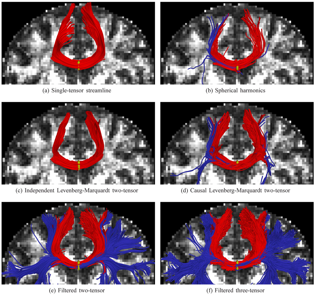
To begin studying the microstructure of fibers, we need a model to interpret the diffusion weighted signal. Such models fall broadly into two categories: parametric and nonparametric. One of the simplest parametric models is the diffusion tensor which describes a Gaussian estimate of the diffusion orientation and strength at each voxel. While robust, this model can be inadequate in cases of mixed fiber presence or more complex orientations [1], [2]. To handle more complex diffusion patterns, various parametric models have been introduced including mixtures of tensors [3]–[7] and directional functions [8]–[10]. To demonstrate the difference that arises among various models, Fig. 1 shows a tracing from the center of the corpus callosum. While a single-tensor model finds only the dominant U-shaped structure, multi-fiber methods reveal many of the lateral pathways known to exist. With such models care must be taken in fitting the model parameters to data, for example, one must determine the number of components present in a particular voxel [11]. As we demonstrate in this paper, incorporating information from neighboring voxels aids in this process [12].

Fig. 1.

Single-tensor tractography misses many of the lateral branches from the corpus callosum. The proposed two-tensor tractography is able to resolve many of these transcallosal pathways. Seed region indicated with yellow.

Nonparametric models often provide more information about the diffusion pattern. Instead of estimating a discrete number of fibers as in parametric models, nonparametric techniques estimate an oriented distribution function (ODF) describing an arbitrary configuration of fibers. For this estimation, [13] introduced Q-ball imaging to numerically compute the ODF via the Funk-Radon transform, and subsequently, the use of spherical harmonics simplified the computation with an analytic form [14]–[16]. Recently, [17] demonstrated online direct estimation of single-tensor and harmonic coefficients using a linear Kalman filter. Another approach to producing an ODF is to assume a model for the signal response of a single-fiber and use spherical deconvolution [9], [18]–[21]. Diffusion oriented transforms offer even another alternative [22]. A good review of both parametric and nonparametric models can be found in [23], [24].

Based on these models, several techniques attempt to reconstruct pathways. Deterministic tractography involves directly following the diffusion pathways. In the single tensor model, this means simply following the principal diffusion direction [25], while multi-fiber models often include techniques for determining the number of fibers present or when pathways branch [6], [26], [27]. Kalman and particle filters have been used with single tensor streamline tractography [28]–[30], but until now these have been used primarily for path regularization. This present work proposes a filtering strategy that propagates the full diffusion model. Another approach to regularizing single-tensor tractography uses a moving least squares estimate weighted with the previous tensor [31]. Probabilistic tractography has been developed as an alternative to deterministic path tracings. These typically form probabilistic notions of connectivity based on sampling individual paths, an approach that begins to quantify the uncertainty of connections [11], [32]–[34]. Building on these local modeling techniques, a third class of algorithms has recently emerged that attempt to optimize the fiber path instead of just the local models [35]–[37].

While parametric methods directly describe the principal diffusion directions, interpreting the ODFs from model independent representations typically involves determining the number and orientation of principal diffusion directions present [38]–[40]. For example, one approach is to deconvolve with a sharpening kernel before extracting maxima [24], while another approach is to decompose a high-order tensor into a mixture of rank-1 tensors [41].

A. Our contributions

Of the approaches listed above, nearly all fit the model at each voxel independent of other voxels; however, tractography is a causal process: we arrive at each new position along the fiber based upon the diffusion found at the previous position. In this paper, we treat model estimation and tractography as such by placing this process within a causal filter. As we examine the signal at each new position, the filter recursively updates the underlying local model parameters, provides the variance of that estimate, and indicates the direction in which to propagate tractography.

To begin estimating within a finite dimensional filter, we model the diffusion signal using a mixture of either two or three Gaussian tensors. This enables estimation directly from the raw signal data without separate preprocessing or regularization steps. Because the signal reconstruction is nonlinear, we use the unscented Kalman filter to estimate the model parameters and then propagate in the most consistent direction. Using causal estimation in this way yields inherent path regularization and accurate fiber resolution at crossing angles not found with independent optimization. We further note that the approach presented here generalizes to arbitrary fiber model with finite dimensional parameter space.

II. APPROACH

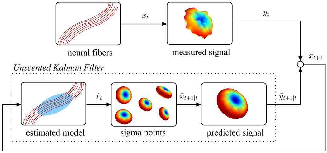
The main idea of our approach is to trace the local fiber orientations using the estimation at previous positions to guide estimation at the current position. In a loop, the Kalman filter estimates the model at the current position, moves a step in the most consistent direction, and then begins estimation again (Fig. 2). Recursive estimation in this manner greatly improves the accuracy of resolving individual orientations and yields inherently smooth tracts despite the presence of noise and uncertainty. Further, since each iteration begins with a near-optimal solution provided by the previous estimation, the convergence of model fitting is improved and many local minima are naturally avoided.

Fig. 2.

System overview illustrating relation between the neural fibers, the scanner signals, and the unscented Kalman filter as it is used to estimate the local model. At each step, the filter uses its current model state (x_t) to predict the observed scanner signal (ȳ_t+1|t) and then compares that against the actual measured signal (y_t) from the scanner in order to update its internal model state (x_t+1).

Section II-A provides the necessary background on modeling the measurement signal using tensors and defines the specific fiber model employed in this study. Then, Section II-B describes how this model may be estimated using an unscented Kalman filter.

A. Modeling local fiber orientations

In diffusion weighted imaging, image contrast is related to the strength of water diffusion, and our goal is to accurately relate these signals to an underlying model of fiber orientation. At each image voxel, diffusion is measured along a set of distinct gradients, u₁,…, u_n ∈ 𝕊² (on the unit sphere), producing the corresponding signal, s = [s₁, …, s_n]^T ∈ ℝⁿ. For voxels containing a mixed diffusion pattern, a general weighted formulation may be written as,

$$s_i=s_0{\displaystyle \sum _j{w}_j{e}^{-b{\mathbf{u}}_i^T{D}_j{\mathbf{u}}_i},}$$ (1)

where s₀ is a baseline signal intensity, b is an acquisition-specific constant, w_j are convex weights, and D_j is a tensor matrix describing a diffusion pattern.

From that general mixture model, we choose to start with two components. This choice is guided by several previous studies which found two-fiber models to be sufficient at b = 1000 [4], [6], [7], [11], [27], [38]. Also, we assume the shape of each tensor to be ellipsoidal, i.e. there is one dominant principal diffusion direction m with eigenvalue λ₁ and the remaining orthonormal directions have equal eigenvalues λ₂ = λ₃ (as in [5], [7], [9], [42]). Last, as in the study of [38], we fix the weights so that each component contributes equally. While assuming equally-weighted compartments may limit flexibility, we found that the eigenvalues adjust to fit the signal in much the same way a fully weighted model would adjust. We will revisit this in the experiments and discussion (Section III-D).

These assumptions then leave us with the following model used in this study:

$$s_i=\frac{s_0}{2}{e}^{-b{\mathbf{u}}_i^T{D}_1{\mathbf{u}}_i}+\frac{s_0}{2}{e}^{-b{\mathbf{u}}_i^T{D}_2{\mathbf{u}}_i},$$ (2)

where D₁, D₂ are each expressible as, D = λ₁mm^T + λ₂(pp^T + qq^T), with m, p, q ∈ 𝕊² forming an orthonormal basis aligned to the principal diffusion direction m. The free model parameters are then m₁, λ₁₁, λ₂₁, m₂, λ₁₂, and λ₂₂. In our current implementation, we restrict each λ to be positive. Extending off the two-tensor model, we can directly formulate a three-tensor version:

$$s_i=\frac{s_0}{3}{\displaystyle \sum _{j=1}^3{e}^{-b{\mathbf{u}}_i^T{D}_{\mathrm{j}}{\mathbf{u}}_i}},$$ (3)

with the additional parameters m₃, λ₁₃, and λ₂₃.

B. Estimating the fiber model

Given the measured scanner signal at a particular voxel, we want to estimate the underlying model parameters that explain this signal. As in streamline tractography, we treat the fiber as the trajectory of a particle which we trace out. At each step, we examine the measured signal at that position, estimate the underlying model parameters, and propagate forward in the most consistent direction, i.e. the component direction most aligned with the incoming vector. Fig. 2 illustrates this filtering process.

To use a state-space filter for estimating the model parameters, we need the application-specific definition of four filter components:

1. The system state x: the model parameters

2. The state transition f[·]: how the model changes as we trace the fiber

3. The observation h[·]: how the signal appears given a particular state

4. The measurement y: the actual signal obtained from the scanner

For our state, we directly use the model parameters, thus the two-fiber model in Eq. 2 has the following state vector:

$$\mathbf{x}={[{\mathbf{m}}_1{\mathrm{\lambda }}_{1_1}{\mathrm{\lambda }}_{2_1}{\mathbf{m}}_2{\mathrm{\lambda }}_{1_2}{\mathrm{\lambda }}_{2_2}]}^T,$$ (4)

where m ∈ 𝕊² and ℝ⁺. Similarly, the three-tensor model adds additional state variables for the third component:

$$\mathbf{x}={[{\mathbf{m}}_1{\lambda }_{1_1}{\lambda }_{2_1}{\mathbf{m}}_2{\lambda }_{1_2}{\lambda }_{2_2}{\mathbf{m}}_3{\lambda }_{1_3}{\lambda }_{2_3}]}^T.$$ (5)

For the state transition we assume identity dynamics; the local fiber configuration does not undergo drastic change from one position to the next. Our observation is the signal reconstruction, y = s = [s₁, …, s_n ]^T using s_i from Eq. 2, and our measurement is the actual signal interpolated directly from the diffusion weighted images at the current position.

Since the signal reconstruction is a nonlinear process, we employ an unscented Kalman filter to perform nonlinear estimation. Similar to classical linear Kalman filtering, the unscented version seeks to reconcile the predicted state of the system with the measured state and addresses the fact that those two processes–prediction and measurement–may be nonlinear or unknown. It does this in two phases: first it uses the system transition model to predict the next state and observation, and then it uses the new measurement to correct that state estimate. In what follows, we present the algorithmic application of the filter. For more thorough treatments, see [43], [44].

It is important to note that while particle filters are a common approach to nonlinear estimation, we chose instead the unscented Kalman filter primarily for its low computational complexity. With respect to state dimension, particle filters require the number of particles to be exponential to properly explore the state space. In contrast, for a Gaussian estimate of the n-dimensional state, the unscented filter requires a linear number of particles (2n + 1 sigma points).

Suppose the system of interest is at time t and we have a Gaussian estimate of its current state with mean, x_t ∈ ℝⁿ, and covariance, P_t ∈ ℝ^{n × n}. Prediction begins with the formation of a set X_t = {χ_i} ⊂ ℝⁿ of 2n + 1 sigma point states with associated convex weights, w_i ∈ ℝ, spread around the current state. We use the covariance, P_t, to distribute this set:

$$\begin{array}{c}\hfill {\chi }_0={\mathbf{x}}_t{w}_0=\kappa /(n+\kappa )w_i=w_{i+n}=\frac{1}{2(n+\kappa )}\hfill \\ \hfill {\chi }_i={\mathbf{x}}_t+{\left[\sqrt{(n+\kappa )P_t}\right]}_i{\chi }_i+n={\mathbf{x}}_t-{\left[\sqrt{(n+\kappa )P_t}\right]}_i\hfill \end{array}$$ (6)

where [A]i denotes the i^th column of matrix A and κ is an adjustable scaling parameter (κ = 0.01 in all experiments). Next, this set is propagated through the state transition function, χ̂ = f[χ] ∈ ℝⁿ, to obtain a new predicted sigma point set: X_t+1|t = {f[χ_i]} = {χ̂_i}. Since in this study we assume the fiber configuration does not change drastically as we follow it from one voxel to the next, we may write this identity transition as, x_t+1|t = f[x_t] = x_t. These are then used to calculate the predicted system mean state and covariance,

$$\begin{array}{c}\hfill {\overline{\mathbf{x}}}_{t+1|t}={\displaystyle \sum _i{w}_i{\widehat{\chi }}_i,}\hfill \\ \hfill P_{xx}={\displaystyle \sum _i{w}_i({\widehat{\chi }}_i-{\overline{\mathbf{x}}}_{t+1|t}){({\widehat{\chi }}_i-{\overline{\mathbf{x}}}_{t+1|t})}^T+Q,}\hfill \end{array}$$ (7)

where Q is the injected process noise bias used to ensure a non-null spread of sigma points and a positive-definite covariance. This procedure comprises the unscented transform used to estimate the behavior of a nonlinear function: spread sigma points based on your current uncertainty, propagate those using your transform function, and measure their spread.

To obtain the predicted observation, we again apply the unscented transform this time using the predicted states, X_t+1|t, to estimate what we expect to observe from the hypothetical measurement of each state: γ = h[χ̂] ∈ ℝ^m. Keep in mind that, for this study, our observation is the signal reconstruction from Eq. 2, and the measurement itself is the diffusion-weighted signal, s, interpolated at the current position. From these, we obtain the predicted set of observations, Y_t+1|t = {h[χ̂_i]} = {γ_i}, and may calculate its weighted mean and covariance,

$${\overline{\mathbf{y}}}_{t+1|t}={\displaystyle \sum _i{w}_i{\widehat{\gamma }}_i,}$$

Algorithm 1.

Main loop repeated for each fiber

1:	repeat
2:	Form the sigma points Xt around xt
3:	Predict the new sigma points Xt+1|t and observations Yt+1|t
4:	Compute weighted means and covariances, e.g. x̄t+1|t, Pxy
5:	Update estimate (xt+1, Pt+1) using scanner measurement (yt)
6:	Proceed in most consistent direction mj
7:	until estimated model appears isotropic

$$P_{yy}={\displaystyle \sum _i{w}_i({\widehat{\gamma }}_i-{\overline{\mathbf{y}}}_{t+1|t}){({\widehat{\gamma }}_i-{\overline{\mathbf{y}}}_{t+1|t})}^T+R,}$$ (8)

where R is the injected measurement noise bias again used to ensure a positive-definite covariance. The cross correlation between the estimated state and measurement may also be calculated:

$$P_{xy}={\displaystyle \sum _i{w}_i({\widehat{\chi }}_i-{\overline{\mathbf{x}}}_{t+1|t}){({\widehat{\gamma }}_i-{\overline{\mathbf{y}}}_{t+1|t})}^T.}$$ (9)

As is done in the classic linear Kalman filter, the final step is to use the Kalman gain, $K=P_{xy}{P}_{yy}^{-1}$, to correct our prediction and provide us with the final estimated system mean and covariance,

$${\mathbf{x}}_{t+1}={\overline{\mathbf{x}}}_{t+1|t}+K({\mathbf{y}}_t-{\overline{\mathbf{y}}}_{t+1|t})$$ (10)

$$P_{t+1}=P_{xx}-{KP}_{yy}{K}^T,$$ (11)

where y_t ∈ ℝ^m is the actual signal measurement taken at this time.

C. The algorithm

To summarize the proposed technique, we are using the unscented Kalman filter to estimate the local model parameters as we trace out each fiber. For each fiber, we maintain the position at which we are currently tracing it and the current estimate of its model parameters (mean and covariance). At each iteration of the algorithm, we predict the new state, which in this case is simply identity: x_t+1|t = x_t. Our actual measurement y_t in Eq. 10 is the diffusion-weighted signal, s, recorded by the scanner at this position. At subvoxel positions we interpolate directly on the diffusion-weighted images. With these, we step through the equations above to find the new estimated model parameters, x_t+1. Last, we use first-order forward Euler integration to move a small step in the most consistent of principal diffusion directions, and then we repeat these steps from that new location. Algorithm 1 outlines these steps.

III. EXPERIMENTS

We begin with synthetic experiments to validate our technique against ground truth. After constructing a set of crossing fiber fields, we perform tractography and examine the underlying orientations and branchings (Section III-A). We then turn to more quantitative experiments over a broad range of angles and component weightings, and we confirm that our approach accurately recognizes crossing fibers (Section III-B) and provides a superior estimate of the diffusion process (Section III-C). We then demonstrate estimation of three-fiber crossings (Section III-E). Lastly, we examine a real dataset to demonstrate how causal estimation is able to pick up fibers and branchings known to exist in vivo yet absent using an assortment of other techniques (Section III-F).

Following the experimental method of generating synthetic data found in [20], [24], [41], we pulled from our real data set the 300 voxels with highest fractional anisotropy (FA) and compute the average eigenvalues among these voxels: {1200, 100, 100}µm²/msec (FA=0.91). We generated synthetic MR signals according to Eq. 1 using these eigenvalues to form an anisotropic tensor at b = 1000 s/mm² using 81 gradient directions uniformly spread on the hemisphere. We assume s₀ = 1 and introduce Rician noise (SNR ≈ 5 dB). For extra experiments at b = 3000 and alternative noise levels, one can refer to an earlier conference version of this work [45].

Throughout the experiments, we compare against several techniques selected to represent standard alternative models and fitting procedures. First, we include direct (least-squares) single-tensor estimation and streamline tractography [25]. Despite its limited utility in crossing and branching regions, this technique is widely used in both the clinical and neuroscience communities and provides a baseline for comparison. Second, we use the same two-tensor model from Section II-A but estimate the model parameters using a Levenberg-Marquardt nonlinear least-squares solver. This shows the effect of filtered estimation versus a standard alternative scheme. Such techniques depend largely on the initialization, and so we employ several variants to remove any uncertainty in initialization. For the synthetic experiments, we initialize with the ground truth. For the in vivo experiments, we initialize with the single-tensor estimate [7] which we loosely refer to as “independent” and we initialize with the estimate at the previous position which we refer to as “causal”. Third, we use spherical harmonics for modeling and fiber-ODF sharpening for peak detection (order l = 8, regularization L = 0.006) [20], [24]. This provides a comparison with an independently estimated, model-free representation. Note that this technique is very similar to spherical deconvolution. We will often refer to this method as “sharpened spherical harmonics”.

The unscented Kalman filter conveniently requires few parameters. Specifically, of importance are the matrices for injecting model noise Q and injecting measurement noise R (see Eq. 7and Eq. 8). Fortunately, the relative magnitude of each can be determined off-line from the data itself, and typically these are formulated as diagonal matrices (zeros off the diagonal). The injected model noise governs how much variance is allowed in the model: higher values allow more variation but, pushed too far, could lead to inaccurate estimation. We found roughly q_m ∈ [0.0015, 0.0030] (roughly 2–4°) and qλ ∈ [25, 100] to allow an appropriate amount of angular and diffusive flexibility among our synthetic and in vivo experiments as well as among various other patients and across other scanner protocols we have encountered. The injected measurement noise governs how much variance is expected in the measurement: higher values mean we expect more variance and hence trust our measurement less. This value depends on the level of physical noise present which varies depending on the scanner, protocol, or pre-processing, and so some experimentation may be necessary. However, in all our experiments thus far, we have found r_s ∈ [0.01, 0.03] to quite robust.

A. Synthetic tractography

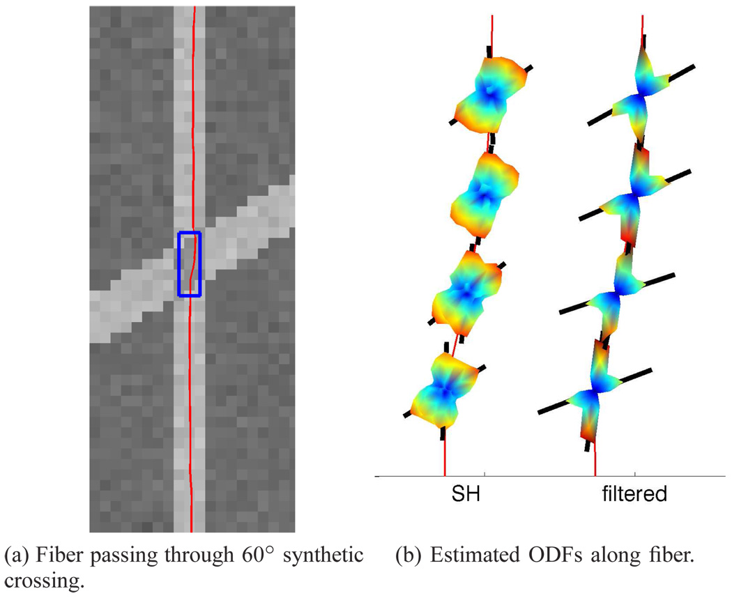
While the independent optimization techniques can be run on individually generated voxels, care must be taken in constructing reasonable scenarios to test the causal filter. For this purpose, we constructed an actual 2D field through which to navigate. In the middle is one long fiber pathway where the filter begins estimating a single tensor but then runs into a field of voxels with two crossed fibers at a fixed angle. We generated several similar fields, each at a different fixed angle and component weighting. In Fig. 3a we show one such field with a 60° crossing. In our experiments, fibers start from the bottom and propagate upward where they encounter the crossing region. We found that in regions with only one true fiber present (those outside the crossing here), the second component consistently aligned with the first.

Fig. 3.

One fiber passing through an example synthetic field and the estimated ODFs within crossing region (blue box) using (unsharpened) spherical harmonics (SH) and the filter. The filter provides consistent angular resolution while SH modeling at those same locations sometimes misses or is off. Above and below the crossing region, the filter aligns both tensor components to fit the single-tensor signal.

In Fig. 3b we take a closer look at several points along this single fiber as it passes through the crossing region. We examine the reconstructed ODFs produced by the filter as well as those produced by spherical harmonic modeling at those same positions. As reported in [24], [41], spherical harmonics at b = 1000 begin to not detect the second component at around 50°-60°, but instead report a single angle as seen in one of the middle samples in Fig. 3b. As reported in [38], [41], [46], a close examination of the reported axes shows this bias toward a single averaged axis. In contrast, the filtered results are consistent and accurate. One can note a slight deflection upon entry of the crossing region as the filter attempts to maintain smooth estimates. The deflection is lessened upon exit since the single component allows for the most stable model fit.

B. Angular resolution

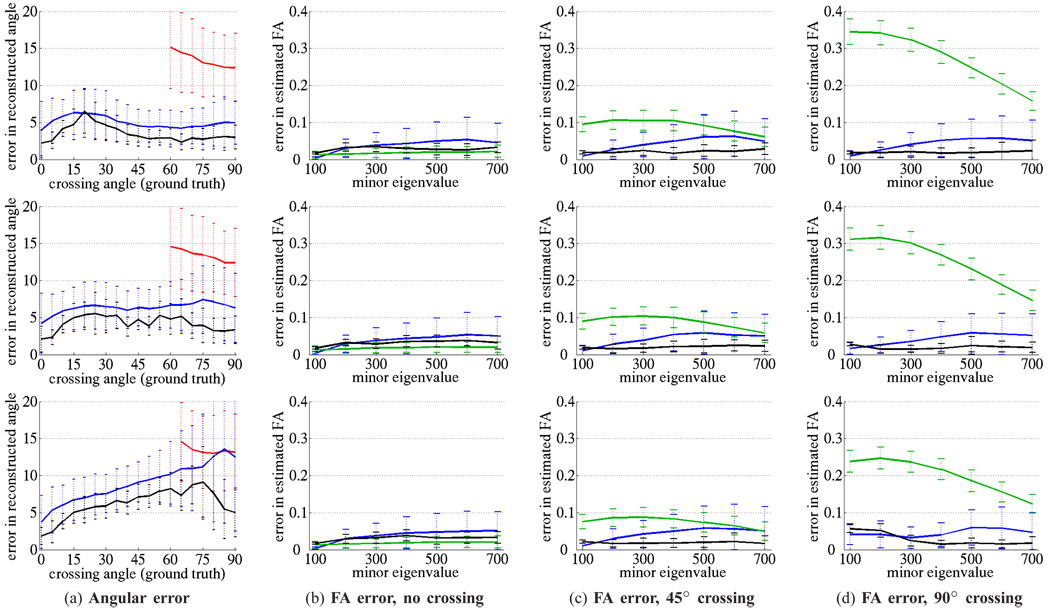
Having verified the underlying behavior, we then began a more comprehensive evaluation and quantified the estimated angle within the crossing regions. Synthetic crossing fields were constructed with a range of crossing angles and weighting combinations. In Fig. 4a each row is a different weighting: top 50–50, middle 60–40, bottom 70–30. Each graph then plots the angular error as a function of crossing angle, from 15° to 90°. Within the crossing regions, we compared the performance among direct single-tensor estimation, sharpened spherical harmonics, a nonlinear solver (Levenberg-Marquardt), and the proposed filter. By varying the size of the crossing regions in Fig. 3a or the number of fibers run, we ensured that each technique performed estimation on at least 500 voxels to produce consistent trendlines across this wide range of angles.

Fig. 4.

The error in estimated crossing angle (a) and estimated fractional anisotropy (b)–(d) at various volume fractions: 50%-50% (top row), 60%-40% (middle row), 70%-30% (bottom row). Where appropriate, we compare among single-tensor least-squares (green), sharpened spherical harmonics (red), two-tensor Levenberg-Marquardt (blue), and the proposed filtered two-tensor (black). Through all examples, the filtered technique provides the most consistent and accurate results.

Fig. 4a shows the estimated separating angle reported using spherical harmonics (red), the nonlinear solver (blue), and the proposed filter (black). Over each technique’s series of estimations, the trendlines indicate the mean error while the bars indicate one standard deviation. Consistent with the synthetic results reported in [16], [24], spherical harmonics are generally unable to detect and resolve angles below 50° for b = 1000 or below 40° for b = 3000. With a perfect initialization, the Levenberg-Marquardt solver is closer to the solution but shows significant variance from the noise. In contrast, the filtered approach statistically estimates the true underlying signal and so is capable of resolving angles down to the range of 20–30° with 5° error in the equally weighted field (50-50) (top row) with performance degrading little in the 60-40 field (middle). In the 70-30 field (bottom), the trendlines begin to show an asymptotic limit to performance, yet the filter is the only method capable of reasonable estimates at large angles. See [45] for additional experiments at both b= 1000 and b = 3000. From these trendlines, one can conclude that the filtered approach provides accurate and consistent angular resolution at crossing angles far below independent estimation.

C. Estimated quantities

While angular resolution is important in accurately resolving paths, the underlying estimated quantities are important in the analysis of these pathways. We focus on three scenarios: a single fiber (no crossing), a 45° crossing, and an orthogonal 90° crossing. In each scenario we hold constant the primary eigenvalue and adjust the minor eigenvalues to produce fields with a range of diffusion properties. Further, we adjust the crossing weights as in the earlier experiments. We compare among the three techniques estimating diffusion quantities: direct single-tensor estimation (green), the two-tensor model with the nonlinear solver (Levenberg-Marquardt initialized with ground truth) (blue), and the two-tensor model with the proposed filter (black). And finally we judge these techniques using the error in estimated fractional anisotropy (FA), one of the most common proxy measures for diffusion.

The fields with a single fiber (no crossing) serve as another baseline. Fig. 4b shows that both direct estimation and the filter provide tight estimates of the true FA. Note the increased variance incurred in the nonlinear solver due to noise. In Fig. 4c, single-tensor estimation begins to show a bias. Levenberg-Marquardt begins to deteriorate slightly, but the filter continues to provide accurate and consistent estimates. Lastly, in Fig. 4d, single-tensor estimation provides erroneous estimates while only the multi-component techniques are able to maintain accuracy. Note again how the filter provides tight estimates.

D. Volume fractions

In the current implementation, we have chosen a model without weights (Eq. 2). To examine this assumption, we included experiments over weighted fields to see the effect on estimation. Each row of Fig. 4 shows a different weighting combination: equal in the top row to most asymmetric in the bottom row.

Despite the equally-weighted assumption, Fig. 4a shows that the filter is capable of correctly resolving angles in the range of 60-40 and only the most orthogonal angles at 70-30. In all of these runs, the filter maintained tracing of the dominant fiber, drifting little in the most asymmetric cases. At 80-20 no technique was able to reliably detect the minor component.

While the filter had trouble picking up the minor component in the more asymmetric cases, Fig. 4b–4d shows that it maintained accurate estimates of the diffusion processes, perhaps the most important consideration. In these regions where the model does not explicitly fit the data, we found that the filter compensates by adjusting the eigenvalues. For example, changes in the eigenvalues could be interpreted as weights: $e^{-b{\mathbf{u}}_i^{T}D{\mathbf{u}}_i}=e^{-b{\mathbf{u}}_i^T(D_a+D_b){\mathbf{u}}_i}=e^{-b{\mathbf{u}}_i^T{D}_a{\mathbf{u}}_i}{e}^{-b{\mathbf{u}}_i^T{D}_b{\mathbf{u}}_i}=w{e}^{-b{\mathbf{u}}_i^T{D}_b{\mathbf{u}}_i}$. In each of the unequally weighted crossings, the filter increases the eigenvalues of the primary component and decreases those of the minor component in order to fit the signal with much the same effect as increasing or decreasing weights. Since all techniques appear to deteriorate beyond the 70-30 weighting, it appears that components of less than 30% contribution will not be reliably detected despite incorporating weights.

The unscented Kalman filter itself places no constraint on the state space except what is statistically likely given the current estimate: all values in the state vector are free to take any value in ℝ. In our current implementation, we restricted m to 𝕊² and λ₁, λ₂ > 0. However, this is an ad hoc solution and we have experimented with applying causal filters capable of estimating under model constraints, e.g. positive eigenvalues, convex weights [47].

E. Three-fiber crossings

Resolving three-fiber crossings has proven difficult for many techniques, especially at the lower b-values typically used in clinical scans. For example, [4] found the general multi-tensor model to be unstable for three or more components using data at b = 1077 with 126 gradients. [48] only reported results for up to two-tensors (b = 700, 30 gradients). In simulation, [11] found that b-values at upwards of 3000–4000 s/mm² were required for detecting more than two fibers and none were found in vivo (b = 1000, 60 gradients). Further, many studies specifically use at most two orientations [3], [6], [7]. However, spherical shell techniques have had some success in resolving three-fiber crossings. [20] reported such crossings using spherical deconvolution (b = 2971, 60 gradients).Most recently, [41] demonstrated tensor decomposition as a promising technique for resolving such configurations (b = 1000, 60 gradients).

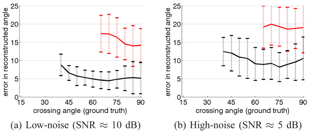
Following the synthetic experimental setup of [41], we constructed an additional set of synthetic fields this time with three equally-weighted Gaussian components. Similar to the synthetic fields shown in Fig. 3a, one fiber is angled up and is the intended orientation to track through the region, but here the other two orientations were set so that the endpoints of the three principal axes formed an equilateral triangle with any two separated by the specified angle. With this setup, Fig. 5 shows that the filtered approach provides an accurate estimate that reaches to roughly 45° compared to 60–65° for spherical harmonics. A significant bias is apparent at more acute angles using either technique.

Fig. 5.

The filtered approach (black) is able to resolve three-fiber crossings with improved accuracy and at sharper angles compared to using sharpened spherical harmonics (red). Both low-noise and high-noise experiments are shown.

F. In vivo tractography

We next test our approach on a real human brain scan acquired on a 3-Tesla GE system using an echo planar imaging (EPI) diffusion weighted image sequence. A double echo option was used to reduce eddy-current related distortions. To reduce impact of EPI spatial distortion, an eight channel coil was used to perform parallel imaging using Array Spatial Sensitivity Encoding Techniques (GE) with a SENSE-factor (speed-up) of 2. Acquisitions have 51 gradient directions with b = 900 and eight baseline scans with b = 0. The original GE sequence was modified to increase spatial resolution, and to further minimize image artifacts. The following scan parameters were used: TR 17000 ms, TE 78 ms, FOV 24 cm, 144×144 encoding steps, 1.7 mm slice thickness. All scans had 85 axial slices parallel to the AC-PC line covering the whole brain. In addition, b=0 field inhomogeneity maps were collected and calculated.

We first focus on fibers originating in the corpus callosum. Specifically, we seek to trace out the lateral transcallosal fibers that run through the corpus callosum out to the lateral gyri. It is known that single-tensor streamline tractography only traces out the dominant pathways forming the U-shaped callosal radiation (Fig. 1, 6a, and 7a). Several studies document this phenomena, among them the works of Descoteaux, Schultz, et al. [24], [41] have side-by-side comparisons. These fibers have been reported in using diffusion spectrum imaging [26], probabilistic tractography [9], [24], [49], and more recently with tensor decomposition [41].

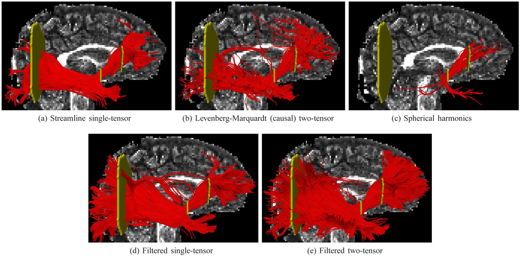
Fig. 6.

Tractography using various methods, seeded at the center of the corpus callosum. Single-tensor reconstructs only the dominate callosal radiata (a). Spherical harmonics pick up some of the lateral branches (b). Initializing a Levenberg-Marquardt solver with an independent single tensor estimate finds only the radiata (c), while initializing instead with its previous estimate (d) finds little more than spherical harmonics. Only filtered tractography picks up the lateral paths consistent with the underlying anatomy. Fibers exiting ±22mm around the mid-sagittal plane are indicated in blue. Seed region indicated in yellow.

Fig. 7.

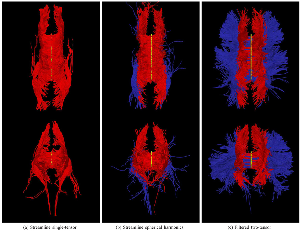
Tracing fibers originating from the center of the entire corpus callosum with views from above (top rows) and front-to-back (bottom rows). The proposed filtered tractography is able to find many of the lateral projections (blue) while single-tensor is unable to find any and few are found with sharpened spherical harmonics. Seed region indicated in yellow.

We start with two basic experiments: first examining the tracts surrounding a single coronal slice and second looking at all tracts passing through the corpus callosum. We seed each algorithm multiple times in voxels at the intersection of the mid-sagital plane and the corpus callosum. We terminate fibers when the generalized fractional anisotropy of the estimated signal (std/rms) fell below 0.1. To explore branchings found using the proposed technique, we consider a component to be branching if it was separated from the primary component by less than 40° with FA ≥ 0.15. Similarly, with sharpened spherical harmonics, we consider it a branch if we find additional maxima over the same range. Unless otherwise stated, in all experiments we follow the primary fiber from the seeding and its branches, i.e. one level of branching. We do not go on to follow the branches on those secondary fibers. While such heuristics are somewhat arbitrary, we found little qualitative difference in adjusting these thresholds.

To demonstrate the flexibility of the proposed filtering strategy with respect to model choice, we use both the two-tensor fiber model (Eq. 2) and the three-tensor fiber model (Eq. 3). While this introduced differences in the quantity of branchings detected, we found that using either model resulted in generally the same pathways. This suggests that the filtering itself accounted for most of the differences compared to the other techniques, more so than the choice of two or three components in the fiber model. Further, it is important to note that despite the more complicated multi-fiber models, the filter provides stable and consistent estimates of the appropriate number of compartments. For example, when tracing using the two-tensor fiber through a one-tensor region, the filter overlaps both tensors to fit the signal (above and below the crossing region in Fig. 3a).

For the first experiment, Fig. 6 shows tracts originating from within a few voxels intersecting a particular coronal slice. As a reference, we use a coronal slice showing the intensity of fractional anisotropy (FA) placed a few voxels behind the seeded coronal position. Keeping in mind that these fibers are intersecting or are in front of the image plane, this roughly shows how the fibers navigate the areas of high anisotropy (bright regions). Comparable to the results in [24], [41], Fig. 6b shows that sharpened spherical harmonics only pick up a few fibers intersecting the U-shaped callosal radiata. In contrast, our proposed method traces out many pathways consistent with the apparent anatomy using either the two-fiber or three-fiber model. To emphasize transcallosal tracts, we color as blue those fibers exiting a corridor of ±22 mm around the mid-sagittal plane. To explore the maximum connectivity found using each approach, this is the one experiment where we followed secondary branches, i.e. primary fibers, their branches, and finally branches off those fibers. Fig. 7 shows a view of the whole brain to see the overall difference between the different methods.

We next combined the filtered tracings from the corpus callosum with those from the internal capsule to demonstrate practically how the filter is able to push through areas of crossing. Fig. 8 shows successive snapshots as two-tensor filtered tracings from the corpus callosum (red) infiltrate those originating in the internal capsule (yellow). Since other methods were unable to reconstruct such dense penetration, it is our hope that this method of multi-tensor tractography will provide rich information in connectivity studies. Fig. 9 takes a closer look at one area where these fiber pathways merge and shows fragments from the fibers traversing through this region using the three-tensor model.

Fig. 8.

Successive snapshots of filtered two-tensor tracing from both the corpus callosum (red) and internal capsule (yellow), viewed from right hemisphere. Here we see the lateral pathways from the corpus cross the motor tracts from the internal capsule.

Fig. 9.

The three-tensor filtered approach is able to trace through this intersection of the corticospinal tract (blue), corpus callosum (red), and superior longitudinal fasciculus (green).

In the experiments thus far, the decision to branch is somewhat ad hoc. An alternative approach to avoid such thresholds is to perform full-brain tractography following only one path and then select fibers using masks. Along these lines we seeded every voxel with FA ≥ 0.15 using each technique discussed so far. In addition, we included filtered single-tensor tractography to contrast to the baseline single-tensor streamline.

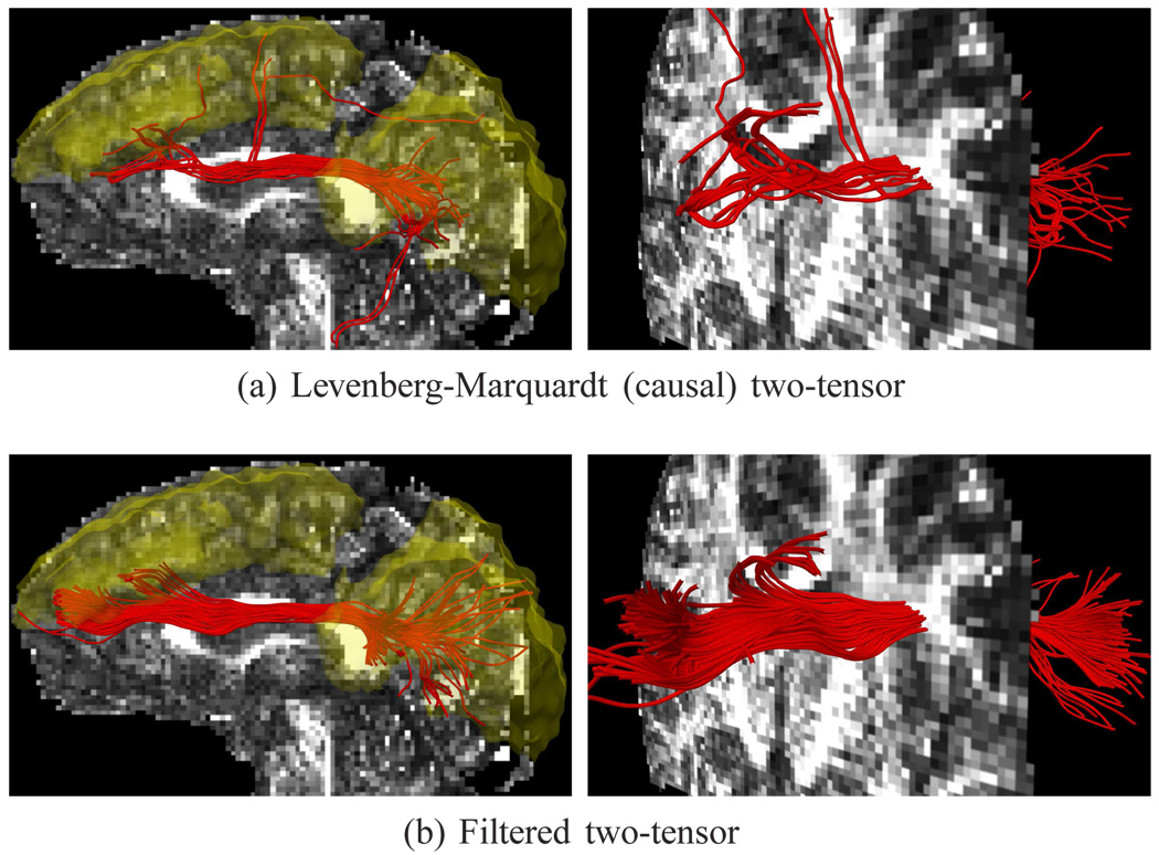
We select out three well-studied pathways. Fig. 10 shows the first pathway, a portion of the superior longitudinal fasciculus as it crosses the lateral pathways exposed in earlier figures. Only two techniques were able to produce this portion of the tract: the causal variant of Levenberg-Marquardt (initializes each step with previous solution) and filtered two-tensor tractography. Both share the same general shape, but the filtered version appears to show a superior reconstruction, especially where the endpoints insert. Spherical harmonics were unable to traverse through the lateral crossings here likely due to ambiguous peaks along this corridor, and the single-tensor models are inherently incapable of modeling the crossing.

Fig. 10.

A portion of the superior longitudinal fasciculus as it crosses a section of the lateral pathways emanating from the corpus callosum. These fibers were extracted using two regions of interest (yellow). While LM reconstructs several of these fibers, filtered estimation produces a more consistent bundle with deeper, uniform penetration into the frontal and occipital lobes. No such fibers were found using the comparison methods.

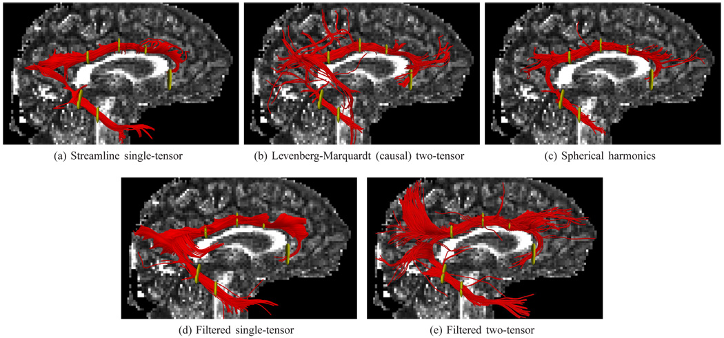
Fig. 11 shows the second pathway, the cingulum bundle as it passes through several gates (yellow). Each technique incurs false-positive fibers at the ends of the corpus–the genu (anterior) and splenium (posterior)–where partial voluming often leads to fibers straying onto the corpus callosum. While all techniques have difficulty making the posterior bend, they begin to differ in their reconstructions of the main body. Going from streamline single-tensor to filtered single-tensor, we see a fuller reconstruction. Levenberg-Marquardt shows many false positives as it easily finds incorrect minima. Sharpened spherical harmonics provide an accurate although sparse reconstruction. Filtered two-tensor provides a full reconstruction although it produces many false positives.

Fig. 11.

Tracing of the right cingulum bundle using various methods. From full-brain seeding, fibers were selected that passed through any two gates (yellow). While all methods here produce some false-positives (e.g. partial voluming onto the splenium, genu, or tapetum), the filtered methods appear to produce the fullest cingulum reconstructions.

Last, Fig. 12 shows tracing of the interior occipital-fronto fasciculus as it spreads and inserts into the occipital and temporal lobes. Streamline single tractography reconstructs the central pathway. Only the filtered techniques provide consistently deeper penetration into the gray matter while retaining coherent paths. Further, only the filtered version of the two-tensor model reconstructs the known minor insertions into the temporal lobe. This is even more pronounced in the views from above in Fig. 13.

Fig. 12.

Tracing of the right inferior fronto-occipital fasciculus using various methods. From full-brain seeding, fibers were selected that passed through any two gates (yellow). Spherical harmonics and Levenberg-Marquardt show sparse and irregular connectivity. Filtered single- and two-tensor results appear to have deeper and more uniform penetration into the occipital lobe.

Fig. 13.

A view of the previous figure from above. Note the consistent deeper penetration of the filtered techniques. The two-tensor method infiltrates many minor pathways into the temporal lobe.

IV. CONCLUSION

Studies involving deterministic tractography rely on the underlying model estimated at each voxel as well as the reconstructed pathways. Most of the work on deterministic and probabilistic tractography has involved estimating the fiber-ODF independently at each voxel and performing tractography as a post-processing step with path regularization. In this work, we proposed a method for simultaneous estimation and tractography using two- and three-tensor mixtures. Using an unscented Kalman filter provided robust parameter estimation and demonstrated significantly higher angular accuracy compared to various nonparametric and independent optimization techniques. Specifically we found an angular error of 5–10° in regions with fiber crossings compared to 15–20° using a common spherical harmonic technique, and it is able to reliably resolve crossings down to 20–30° compared to spherical harmonics which reaches only down to 50‱60°. In vivo experiments demonstrate the ability of the proposed method to reveal fibers known to exist anatomically, e.g. lateral transcallosal fibers or temporal insertions along the fronto-occipital fasciculus, yet absent using the comparison techniques.

Nevertheless, there are several aspects of this technique that could be improved in future work. First, we believe improvements can certainly be made with the local model. For example, switching filters may provide a natural method for reduced parameter estimation where appropriate. Further, we believe it is still important to explore constrained models (convex weights, positive eigenvalues) [47] as well as approaches at model selection [11].

Second, as is often the case in tractography, reported connections may be invalid (false-positives). For example, the partial voluming along the cingulum bundle in Fig. 11 causes many spurious traces. There are several possible approaches to suppressing such false positives (e.g. higher resolution scans, more appropriate local models, alternative filter formulations), but we believe that incorporating global information will ultimately have more effect than more local choices in the model or filter.

In summary, we believe that filtering techniques offer significant increases in sensitivity over traditional independent optimization methods, but care must be taken ensuring anatomically correct results. We believe that exploring both alternative models and filtering techniques will provide more accurate and comprehensive information about neural pathways and ultimately enhance non-invasive diagnosis and treatment of brain disease.

REFERENCES

- 1.Alexander DC, Barker G, Arridge S. Detection and modeling of non-Gaussian apparent diffusion coefficient profiles in human brain data. Magnetic Resonance in Medicine. 2002;vol. 48:331–340. doi: 10.1002/mrm.10209. [DOI] [PubMed] [Google Scholar]
- 2.Frank L. Characterization of anisotropy in high angular resolution diffusion-weighted MRI. Magnetic Resonance in Medicine. 2002;vol. 47:1083–1099. doi: 10.1002/mrm.10156. [DOI] [PubMed] [Google Scholar]
- 3.Alexander A, Hasan K, Tsuruda J, Parker D. Analysis of partial volume effects in diffusion-tensor MRI. Magnetic Resonance in Medicine. 2001;vol. 45:770–780. doi: 10.1002/mrm.1105. [DOI] [PubMed] [Google Scholar]
- 4.Tuch D, Reese T, Wiegell M, Makris N, Belliveau J, Wedeen V. High angular resolution diffusion imaging reveals intravoxel white matter fiber heterogeneity. Magnetic Resonance in Medicine. 2002;vol. 48:577–582. doi: 10.1002/mrm.10268. [DOI] [PubMed] [Google Scholar]
- 5.Parker G, Alexander DC. Probabilistic anatomical connectivity derived from the microscopic persistent angular structure of cerebral tissue. Phil. Trans. R. Soc. B. 2005;vol. 360:893–902. doi: 10.1098/rstb.2005.1639. [DOI] [PMC free article] [PubMed] [Google Scholar]
- 6.Kreher B, Schneider J, Mader I, Martin E, Hennig J, Il’yasov K. Multitensor approach for analysis and tracking of complex fiber configurations. Magnetic Resonance in Medicine. 2005;vol. 54:1216–1225. doi: 10.1002/mrm.20670. [DOI] [PubMed] [Google Scholar]
- 7.Peled S, Friman O, Jolesz F, Westin C-F. Geometrically constrained two-tensor model for crossing tracts in DWI. Magnetic Resonance in Medicine. 2006;vol. 24(no. 9):1263–1270. doi: 10.1016/j.mri.2006.07.009. [DOI] [PMC free article] [PubMed] [Google Scholar]
- 8.McGraw T, Vemuri B, Yezierski B, Mareci T. Von Mises-Fisher mixture model of the diffusion ODF. Int. Symp. on Biomedical Imaging. 2006:65–68. doi: 10.1109/ISBI.2006.1624853. [DOI] [PMC free article] [PubMed] [Google Scholar]
- 9.Kaden E, Knøsche T, Anwander A. Parametric spherical deconvolution: Inferring anatomical connectivity using diffusion MR imaging. NeuroImage. 2007;vol. 37:474–488. doi: 10.1016/j.neuroimage.2007.05.012. [DOI] [PubMed] [Google Scholar]
- 10.Rathi Y, Michailovich O, Shenton ME, Bouix S. Directional functions for orientation distribution estimation. Medical Image Analysis. 2009;vol. 13:432–444. doi: 10.1016/j.media.2009.01.004. [DOI] [PMC free article] [PubMed] [Google Scholar]
- 11.Behrens T, Johansen-Berg H, Jbabdi S, Rushworth M, Wool-rich M. Probabilistic diffusion tractography with multiple fibre orientations: What can we gain? NeuroImage. 2007;vol. 34:144–155. doi: 10.1016/j.neuroimage.2006.09.018. [DOI] [PMC free article] [PubMed] [Google Scholar]
- 12.King MD, Gadian DG, Clark CA. A random effects modeling approach to the crossing-fibre problem in tractography. NeuroImage. 2009;vol. 44:753–768. doi: 10.1016/j.neuroimage.2008.09.058. [DOI] [PubMed] [Google Scholar]
- 13.Tuch D. Q-ball imaging. Magnetic Resonance in Medicine. 2004;vol. 52:1358–1372. doi: 10.1002/mrm.20279. [DOI] [PubMed] [Google Scholar]
- 14.Anderson A. Measurement of fiber orientation distributions using high angular resolution diffusion imaging. Magnetic Resonance in Medicine. 2005;vol. 54(no. 5):1194–1206. doi: 10.1002/mrm.20667. [DOI] [PubMed] [Google Scholar]
- 15.Hess C, Mukherjee P, Han E, Xu D, Vigneron D. Q-ball reconstruction of multimodal fiber orientations using the spherical harmonic basis. Magnetic Resonance in Medicine. 2006;vol. 56:104–117. doi: 10.1002/mrm.20931. [DOI] [PubMed] [Google Scholar]
- 16.Descoteaux M, Angelino E, Fitzgibbons S, Deriche R. Regularized, fast, and robust analytical Q-ball imaging. Magnetic Resonance in Medicine. 2007;vol. 58:497–510. doi: 10.1002/mrm.21277. [DOI] [PubMed] [Google Scholar]
- 17.Poupon C, Roche A, Dubois J, Mangin J-F, Poupon F. Real-time MR diffusion tensor and Q-ball imaging using Kalman filtering. Medical Image Analysis. 2008;vol. 12(no. 5):527–534. doi: 10.1016/j.media.2008.06.004. [DOI] [PubMed] [Google Scholar]
- 18.Jian B, Vemuri B. A unified computational framework for deconvolution to reconstruct multiple fibers from diffusion weighted MRI. Trans. on Med. Imag. 2007;vol. 26(no. 11):1464–1471. doi: 10.1109/TMI.2007.907552. [DOI] [PMC free article] [PubMed] [Google Scholar]
- 19.Jansons K, Alexander DC. Persistent angular structure: New insights from diffusion MRI data. Inverse Problems. 2003;vol. 19:1031–1046. doi: 10.1007/978-3-540-45087-0_56. [DOI] [PubMed] [Google Scholar]
- 20.Tournier J-D, Calamante F, Gadian D, Connelly A. Direct estimation of the fiber orientation density function from diffusion-weighted MRI data using spherical deconvolution. NeuroImage. 2004;vol. 23:1176–1185. doi: 10.1016/j.neuroimage.2004.07.037. [DOI] [PubMed] [Google Scholar]
- 21.Kumar R, Barmpoutis A, Vemuri BC, Carney PR, Mareci TH. Multi-fiber reconstruction from DW-MRI using a continuous mixture of von Mises-Fisher distributions. Mathematical Methods in Biomedical Image Analysis (MMBIA) 2008:1–8. [Google Scholar]
- 22.Özarslan E, Shepherd T, Vemuri B, Blackband S, Mareci T. Resolution of complex tissue microarchitecture using the diffusion orientation transform. NeuroImage. 2006;vol. 31(no. 3):1086–1103. doi: 10.1016/j.neuroimage.2006.01.024. [DOI] [PubMed] [Google Scholar]
- 23.Alexander DC. Multiple-fiber reconstruction algorithms for diffusion MRI. Annals of the New York Academy of Sciences. 2005;vol. 1046(no. 1):113–133. doi: 10.1196/annals.1340.018. [DOI] [PubMed] [Google Scholar]
- 24.Descoteaux M, Deriche R, Knoesche T, Anwander A. Deterministic and probabilistic tractography based on complex fiber orientation distributions. Trans. on Med. Imag. 2009;vol. 28(no. 2):269–286. doi: 10.1109/TMI.2008.2004424. [DOI] [PubMed] [Google Scholar]
- 25.Basser P, Pajevic S, Pierpaoli C, Duda J, Aldroubi A. In vivo fiber tractography using DT-MRI data. Magnetic Resonance in Medicine. 2000;vol. 44:625–632. doi: 10.1002/1522-2594(200010)44:4<625::aid-mrm17>3.0.co;2-o. [DOI] [PubMed] [Google Scholar]
- 26.Hagmann P, Reese T, Tseng W-Y, Meuli R, Thiran J-P, Wedeen VJ. Diffusion spectrum imaging tractography in complex cerebral white matter: An investigation of the centrum semiovale. Int. Symp. on Magnetic Resonance in Medicine (ISMRM) 2004:623. [Google Scholar]
- 27.Guo W, Zeng Q, Chen Y, Liu Y. Using multiple tensor deflection to reconstruct white matter fiber traces with branching. Int. Symp. on Biomedical Imaging. 2006:69–72. [Google Scholar]
- 28.Gössl C, Fahrmeir L, P utz B, Auer L, Auer D. Fiber tracking from DTI using linear state space models: Detectability of the pyramidal tract. NeuroImage. 2002;vol. 16:378–388. doi: 10.1006/nimg.2002.1055. [DOI] [PubMed] [Google Scholar]
- 29.Björnemo M, Brun A, Kikinis R, Westin C-F. Regularized stochastic white matter tractography using diffusion tensor MRI. Medical Image Computing and Computer Assisted Intervention (MICCAI) 2002:435–442. [Google Scholar]
- 30.Zhang F, Hancock E, Goodlett C, Gerig G. Probabilistic white matter fiber tracking using particle filtering and von Mises-Fisher sampling. Medical Image Analysis. 2009;vol. 13:5–18. doi: 10.1016/j.media.2008.05.001. [DOI] [PMC free article] [PubMed] [Google Scholar]
- 31.Zhukov L, Barr A. Oriented tensor reconstruction: Tracing neural pathways from diffusion tensor MRI. Visualization. 2002:387–394. [Google Scholar]
- 32.Parker G, Alexander DC. Probabilistic Monte Carlo based mapping of cerebral connections utilizing whole-brain crossing fiber information. Information Processing in Medical Imaging (IPMI) 2003:684–696. doi: 10.1007/978-3-540-45087-0_57. [DOI] [PubMed] [Google Scholar]
- 33.Hosey T, Williams G, Ansorge R. Inference of multiple fiber orientations in high angular resolution diffusion imaging. Magnetic Resonance in Medicine. 2005;vol. 54:1480–1489. doi: 10.1002/mrm.20723. [DOI] [PubMed] [Google Scholar]
- 34.Iturria-Medina Y, Canales-Rodríguez EJ, Melie-García L, Valdés-Hernández PA, Martńez-Montes E, Alemán-Gómez Y, Sánchez-Bornot JM. Characterizing brain anatomical connections using diffusion weighted MRI and graph theory. NeuroImage. 2007;vol. 36:645–660. doi: 10.1016/j.neuroimage.2007.02.012. [DOI] [PubMed] [Google Scholar]
- 35.Fillard P, Poupon C, Mangin J-F. A novel global tractography algorithm based on an adaptive spin glass model. Medical Image Computing and Computer Assisted Intervention (MICCAI) 2009:927–934. doi: 10.1007/978-3-642-04268-3_114. [DOI] [PubMed] [Google Scholar]
- 36.Jbabdi S, Woolrich M, Andersson J, Behrens T. A Bayesian framework for global tractography. NeuroImage. 2007;vol. 37:116–129. doi: 10.1016/j.neuroimage.2007.04.039. [DOI] [PubMed] [Google Scholar]
- 37.Kreher B, Madeer I, Kiselev V. Gibbs tracking: A novel approach for the reconstruction of neuronal pathways. Magnetic Resonance in Medicine. 2008;vol. 60:953–963. doi: 10.1002/mrm.21749. [DOI] [PubMed] [Google Scholar]
- 38.Zhan W, Yang Y. How accurately can the diffusion profiles indicate multiple fiber orientations? A study on general fiber crossings in diffusion MRI. J. of Magnetic Resonance. 2006;vol. 183:193–202. doi: 10.1016/j.jmr.2006.08.005. [DOI] [PubMed] [Google Scholar]
- 39.Seunarine K, Cook P, Hall M, Embleton K, Parker G, Alexander DC. Exploiting peak anisotropy for tracking through complex structures. Mathematical Methods in Biomedical Image Analysis (MMBIA) 2007:1–8. [Google Scholar]
- 40.Jian B, Vemuri B, Özarslan E, Carney PR, Mareci TH. A novel tensor distribution model for the diffusion-weighted MR signal. NeuroImage. 2007;vol. 37(no. 1):164–176. doi: 10.1016/j.neuroimage.2007.03.074. [DOI] [PMC free article] [PubMed] [Google Scholar]
- 41.Schultz T, Seidel H. Estimating crossing fibers: A tensor decomposition approach. Trans. on Visualization and Computer Graphics. 2008;vol. 14(no. 6):1635–1642. doi: 10.1109/TVCG.2008.128. [DOI] [PubMed] [Google Scholar]
- 42.Friman O, Farnebäck G, Westin C-F. A Bayesian approach for stochastic white matter tractography. Trans. on Med. Imag. 2006;vol. 25(no. 8):965–978. doi: 10.1109/tmi.2006.877093. [DOI] [PubMed] [Google Scholar]
- 43.Julier S, Uhlmann J. Unscented filtering and nonlinear estimation. IEEE. 2004;vol. 92(no. 3):401–422. [Google Scholar]
- 44.van der Merwe R, Wan E. Sigma-point Kalman filters for probabilistic inference in dynamic state-space models. Workshop on Advances in Machine Learning. 2003 [Google Scholar]
- 45.Malcolm JG, Shenton ME, Rathi Y. Neural tractography using an unscented Kalman filter. Information Processing in Medical Imaging (IPMI) 2009:126–138. doi: 10.1007/978-3-642-02498-6_11. [DOI] [PMC free article] [PubMed] [Google Scholar]
- 46.Tournier J-D, Calamante F, Connelly A. Robust determination of the fibre orientation distribution in diffusion MRI: Non-negativity constrained super-resolved spherical deconvolution. NeuroImage. 2007;vol. 35:1459–1472. doi: 10.1016/j.neuroimage.2007.02.016. [DOI] [PubMed] [Google Scholar]
- 47.Malcolm JG, Shenton ME, Rathi Y. Two-tensor tractography using a constrained filter. Medical Image Computing and Computer Assisted Intervention (MICCAI) 2009:894–902. doi: 10.1007/978-3-642-04268-3_110. [DOI] [PMC free article] [PubMed] [Google Scholar]
- 48.Bergmann O, Kindlmann G, Lundervold A, Westin C-F. Diffusion k-tensor estimation from Q-Ball imaging using discretized principal axes. Medical Image Computing and Computer Assisted Intervention (MICCAI) 2006:268–275. doi: 10.1007/11866763_33. [DOI] [PubMed] [Google Scholar]
- 49.Anwander A, Descoteaux M, Deriche R. Probabilistic Q-Ball tractography solves crossings of the callosal fibers. Human Brain Mapping. 2007:342. [Google Scholar]